Deep-based conditional probability density function forecasting of residential loads

(1)

Deep-Based Conditional Probability Density

Function Forecasting of Residential Loads

Mousa Afrasiabi, Mohammad Mohammadi,

Member, IEEE,

Mohammad Rastegar,

Member, IEEE

Lina Stankovic,

Senior Member, IEEE,

Shahabodin Afrasiabi and Mohammad Khazaei

Abstract—This paper proposes a direct model for conditional probability density forecasting of residential loads, based on a deep mixture network. Probabilistic residential load forecasting can provide comprehensive information about future uncertain-ties in demand. An end-to-end composite model comprising convolution neural networks (CNNs) and gated recurrent unit (GRU) is designed for probabilistic residential load forecasting. Then, the designed deep model is merged into a mixture density network (MDN) to directly predict probability density functions (PDFs). In addition, several techniques, including adversarial training, are presented to formulate a new loss function in the direct probabilistic residential load forecasting (PRLF) model. Several state-of-the-art deep and shallow forecasting models are also presented in order to compare the results. Furthermore, the effectiveness of the proposed deep mixture model in char-acterizing predicted PDFs is demonstrated through comparison with kernel density estimation, Monte Carlo dropout, a combined probabilistic load forecasting method and the proposed MDN without adversarial training.

Index Terms—Residential load forecasting, conditional prob-abilistic load forecasting, deep mixture network, convolutional neural network, gated recurrent unit

I. INTRODUCTION A. Motivation

R

ESIDENTIAL customers are increasingly important players in the deregulated distribution networks. They form more than 40% of total energy consumption in 2015, and is expected to grow by 25% in the next ten years, worldwide [1]. Stability and control approaches of modern electricity systems focused on residential loads, such as smart homes, microgrids, and active distribution networks, should be robust to demand variability by combining predicted informa-tion with short/long term scheduling. The ongoing expansion of advanced metering infrastructure (AMI) has created new opportunities for residential customers to participate in the operation of power systems. In this context, the nonlinearity and volatility of the loads strongly influence the forecasting engines [2], [3].

Residential load forecasting (point or probabilistic) is ex-tremely challenging for a single domestic user. Each load profile can be decomposed into three main components, i.e. regular pattern, uncertainty pattern, and noise pattern [3]. Reg-ular pattern is the periodic load component that can be derived M. Afrasiabi, M. Mohammadi, M. Rastegar and S.Afrasiabi are with the School of Electrical and Computer Engineering, Shiraz University, Shiraz, Iran (e-mail: [email protected], [email protected], [email protected]).

L.Stankovic and M.Khazaei are with the Department of Electronic and Electrical Engineering, University of Strathclyde, Glasgow, UK (email: [email protected], [email protected]).

from historical data. Uncertainty patterns are the aperiodic component of the load profile, produced by influential factors e.g. metrological parameters and consumer behavior. The residual of a load profile cannot be physically explained, hence termed the noise component. Current forecasting methods focus on the regular pattern as it is more predictable and makes up a significant proportion of the aggregated load profile. However, a single residential load profile is composed of a larger share of uncertainty, not covered by regular patterns only. To tackle the challenge of significant uncertainty, four different approaches have been proposed in the literature [3]. i) Cluster/classify similar customers in terms of the number of the days/weather to reduce the variance of the uncertainty. The performance of the cluster/classification based approaches are highly dependent on the influential information, ii) Cancel out uncertainties by aggregating residential load data, obtained by multiple smart meters. This is not applicable at a disaggregated level. iii) Using time/frequency domain signal processing, in particular frequency domain analysis such as Fourier or wavelet transforms, to separate uncertainty and noise patterns from the regular patterns. In this case, however, the uncertainty patterns with large share are ignored, iv) Deep Learning methods that can directly learn uncertainties from the raw form.

To the best of our knowledge, the first three approaches tackle the problem indirectly, aiming to mitigate uncertainty by reducing (clustering), cancelling out (aggregation) or filtering out (spectral analysis) the uncertainty. Deep learning, on the other hand, attempts to handle this level of uncertainty by directly learning from the data, and fully capturing its temporal and spatial patterns.

This significant uncertainty pose a significant challenge in effective residential load forecasting. Thus, probabilistic residential-level load forecasting (PRLF) is essential to provide comprehensive information about future load consumption to reduce operation costs and improve the reliability of the smart grid [4]. Probability density function (PDF) can provide full statistical information in future time slots. To directly predict the PDF of residential consumers, a mixture density network (MDN) is selected in this paper. While an MDN is presented in [5] to directly approximate a PDF, the main limitation of this approach is the requirement of a large network, which consists of more than two hidden layers. We propose a deep learning based approach to overcome this problem. Motivated by the performance of deep mixture density network used for stochastic analysis of speech signals in [6], we design a deep mixture network to predict the PDF of residential loads that

(2)

is capable of directly learning uncertainty and spatio-temporal features from the raw load data.

B. Brief Literature Review

Short-term load forecasting methods can be categorized into four main groups, namely persistence, physical, statistical, and artificial intelligence. In persistence models, the load values in forthcoming time intervals are fixed to those of previous time intervals. Persistence methods are highly inaccurate when the period of prediction is more than several hours [7]. Physical models take into account historical data and corresponding meteorological data based on mathematical expressions. For instance, in [8] a physical model based on dynamic empirical model is presented for short-term load forecasting. However, physical models suffer from high computational burden and require memory space [7]. Statistical methods are mostly based on autoregressive methods such as Autoregressive moving average (ARMA) [9] and generalized autoregressive condi-tional heteroskedasticity (GARCH) [10]. Statistical models are usually less complex than physical methods [11]. However, statistical methods are based on linear models while load forecasting is a complex and nonlinear problem. For instance, although the GARCH model is able to capture the uncertainty to some extent, as shown by [7], GARCH models have limited ability to capture non-linear and non-stationary characteristics of volatile time series. In general, the aforementioned statisti-cal methods do not directly capture the uncertainty pattern of a single residential load, but try to reduce this uncertainty using, for example clustering techniques [3]. Artificial intelligence methods have emerged recently since they can learn nonlinear and complex models, do not need any predefined mathematical models, and can be divided into shallow and deep structure-based methods. For instance, artificial neural networks (ANN) [12], support vector machine (SVM) [13], random forest [14], wavelet neural networks [15], and extreme learning machine [16] are shallow-based methods proposed for load forecasting, but they perform poorly in feature mining. Therefore, these methods need additional feature extraction and selection to improve the accuracy. Finding an optimal feature extraction scheme is still a challenging problem [2], [3]. Besides, we cannot generalize these methods to different datasets mainly because of their small hypothesis space due to the small number of parameters [17].

Pre-processing techniques, such as spectral analysis, sepa-rate regular patterns of load profile from uncertainty patterns and noise. However, spectral analyses dramatically degrade the accuracy due to the low proportion of regular patterns in the meter-level loads [3]. Deep structure based methods, known as deep neural networks (DNNs), are able to tackle the aforementioned limitations of shallow-based methods through multiple layer processing and hierarchically learning features from historical raw data. Long short-term memory (LSTM) [2], [3] and convolutional neural network (CNN) [18] are two powerful structures in time series analysis that have been proposed recently. Gated recurrent unit (GRU) is a less complex implementation of LSTM to speed up time series analysis [19], but it is weak in capturing the dependencies of long-tailed raw time series [20]. In addition, CNN is unable

to fully exploit temporal features. In order to address these problems, this paper aims to leverage the advantages of CNN and GRU in a deep mixture structure. Table I summarizes the short-term forecasting methods descriptions, with their pros and cons.

Time series forecasting are implemented as point or prob-abilistic forecasts. Most previous approaches [2], [3], [12]– [16] forecasted the point value in look-ahead times without indicating the associated uncertainty. To accommodate the risk brought by the uncertainty of the meter-level loads, probabilis-tic load forecasting is essential in stochasprobabilis-tic decision making in modern power systems [21]. Probabilistic forecasting was first tackled via Prediction intervals (PIs) methods to construct a set of PIs instead of point values from the future information of time series. In PI methods, firstly, a forecasting method such as neural networks is trained through optimization of an error-based cost function. Then, PIs are constructed for look-ahead times from outputs of the trained forecasting model. The traditional PIs methods, such as delta, Bayesian, bootstrap, bootstrap, and mean-variance are indirect and suffer from high computational cost and poor performance [11]. To tackle this problem, in [22], an interval of the aggregated loads for a microgrid is forecasted based on the fuzzy model in a direct manner. Lower-Upper Band Estimation (LUBE) and deep learning-based simple recurrent neural network (RNN) is used to construct PIs in look-ahead times [11]. LUBE [23] is merged into an ANN and a composite metaheuristic algorithm involving genetic and simulated annealing algorithm to realize the future information about a time series. In these methods, the confidence level is predefined without indicating how to select the appropriate confidence level [24]. In [25], mixed-integer linear programming attempts to fill this gap. MDN is proposed for direct forecasting iin [26] to construct PIs of wind powers. A hierarchical approach based on empirical copulas combines synthesized smart meter data to forecast the upper and lower load bands in [27]. In contrast to PIs, Quantile forecasting methods attempt to construct a set of quantiles instead of PIs. For instance, in [28] wavelet decomposition is used before quantile forest regression and RF as a shallow structure to predict a set of quantiles for network-level loads. Hybrid network models are computationally expensive and signal processing based feature extractors such as wavelet transform are highly sensitive to noise. Hence, selecting the optimal technique for feature extraction still remains unan-swered [3]. The Q-learning dynamic based method of [29] is deterministic and provides a set of quantiles for load forecasting. A comparative study between several benchmarks e.g. an autoregressive model and Holt-Winters-Taylor (HWT) are compared in terms of point and quantile forecasting in [30]. As deep learning-based quantile forecasting, LSTM and CNN are extended via a pinball loss function to extract the quantile in [31] and [32], respectively. PDF forecasting provides full statistical information about load data in look-ahead times by constructing PDFs. PDF forecasting provides more distribution information than a single set of PIs or quantiles [33], [34]. Other forms of probabilistic forecasting, including PIs, quan-tiles and statistical moments, can be derived from the PDFs. A comprehensive review of probabilistic forecasting in [35], [36]

(3)

TABLE I

DIFFERENTMETHODS FORTIMESERIESFORECASTING OFRESIDENTIALLOADS

Persistence Physical Statistical Artificial Intelligence

Description Load in the specific future time intervals is the same as the forecast time

Modeling load time series based on mathematical expres-sions

Modeling based on the difference between the ac-tual time series in immedi-ate past and actual data

Based on learning the feature of the time series through training on historical data Divided into shallow and deep structures

Advantage Good performance in forecasting for ultra-short horizons

Use of meteorological features and good performance in very long horizons

Based on patterns and easy to implement

Ability to capture non-linear and complex models

Disadvantage Unsuitable for regular pre-diction for long horizons

Very high computational bur-den and poor performance in capturing the uncertainty of residential loads profile

Cancels out the uncer-tainty pattern and impre-cise to model the complex and nonlinear time series

Shallow-based structures unable to charac-terize full features without extra feature ex-traction technique, which is unable to han-dle uncertainty pattern of load profile Ex-isting deep learning structures cannot fully learn spatial-temporal features

indicate that, unlike the first two classes of PRLF methods, estimating sophisticated PDF of loads, especially residential loads, is yet to be tackled in depth in the literature. For instance, the parametric ensemble model of extreme learning machine based method and logistic distribution model are presented in [34] to predict the PDF of prices. The nonpara-metric Bayesian-based method of [33] extracts the PDF of wind power for the next few hours. In [37], conditional kernel density (CKD), in combination with a decay parameter, has the ability to predict the smart-level load in density, quantile, and PDF forms in an indirect manner. [38] tackles probabilistic load forecasting using deep residual and Monte-Carlo drop out technique. In [39], based on the Gaussian mixture model, an optimization problem is formulated to construct PDFs of the aggregated loads using continuously ranked probability score as the objective function. These studies are performed in an indirect manner, in which several point forecasts are carried out at first, then a PDF is estimated for future hours. In indirect forecasting structures, the forecasting errors grow with each iteration as the forecasting method propagates the model error, especially when the time series has a significant amount of uncertainty. In [2] and [40], a comprehensive com-parison between different forecasting models demonstrated that forecasting models for individual residential load are imperfect and propagate the large values of error, where MAPE exceeds 21% and 41% in [2] and [40], respectively. To this end, indirect forecasting models can produce large errors in PDF forecasting. Furthermore, we can conclude that point values or even several statistical moments such as median and expected values are not good candidates to describe the uncertainty of residential loads. To tackle these problems, we propose MDN as a potential solution. However, the standard MDN is limited by: leading a loss function to NaN value, poor performance in capturing external features, and large network which consists of more than two hidden layers. In this paper, a loss function is reformulated to prevent a NaN value and is integrated into a deep structure to propose a unique deep mixture neural network capable of directly forecasting the conditional probability of aggregated and disaggregated residential loads.

C. Contributions and Organization

This study aims to build a DNN model from historical data to directly predict the PDF of residential loads based on past time series. A deep mixture density network is selected as a potential solution. We first develop a loss function for the standard MDN to mitigate the possibility of NaN values and enhance the learning ability based on several techniques. In addition to directly learning the severe uncertainty of the residential load, which has a large share in the consumption profile, we propose a structure to fully capture spatio-temporal features from raw data. In the proposed approach, the designed deep mixture network breaks down into CNN, GRU, and fully-connected neural (FCN) layers. CNN learns the spatial features during training, while GRU enhances the capability of capturing temporal characteristics. Consequently, several FCN layers are connected to construct PDFs based on a MDN. The key contributions of this paper are enumerated as follows:

• A deep mixture model designed to directly capture inher-ent intermittinher-ent uncertainty of the residinher-ential load profiles without any cancelation of uncertainty by aggregating the loads or separating out the regular pattern based on raw data.

• Developing a loss function in MDN to avoid NaN values and enhance the learning capability.

• Full statistical information is obtained by predicting PDF at each time interval in a direct procedure to prevent errors that might be propagated by the indirect structure and improve the computational efficiency.

The rest of the paper is organized as follows: The back-ground and the proposed formulation of the loss function are introduced in Section II. Section III describes the training process of the proposed deep mixture density network. In Section IV, the proposed deep mixture structure and the end-to-end model are explained. Numerical results are presented and discussed in Section V before concluding in Section VI.

II. LOSSFUNCTIONREFORMULATION INMDNFOR CONDITIONALLOADFORECASTING

The loss function is an influential factor in the learning ability of time series forecasting that must faithfully distill all aspects of the model down to a single number in such a way

(4)

that improvements in that number are indicative of a better model. In order to directly predict the PDF for future informa-tion, existing loss functions, such as continuously ranked prob-ability score (CRPS) [41] are impractical. The standard MDN attempts to construct PDF-based conditional probability-based loss function also faces a number of challenges, which are resolved in this paper with several modifications.

Let (X, Y) = (x1, y1), ...,(xn, yn) be data, where xi ∈

RI ∀ i =1,...,niis the niinput data andyj∈Ro∀j =1,...,nois

the noobservation space data. The key idea in point forecasting

is to construct a function that projects Y and the forecasted values,yˆwith minimal difference.

Conditional probabilistic forecasting represents (X, Y) as discrete random variables to predict conditional distribution of X given outcome ofY, p(y|x), which usually follows an unknown distribution.

A. Standard MDN

To approximate p(y|x)an ensemble mixture or sum of the number of Gaussian distributions can be used. In conditional probabilistic forecasting, probability density of target yt can

be expressed as a linear combination of kernel functions in the form of:

p(yt|x) = N X n=1 πn(x, t)ϕ(yt|µn(x, t), σn2(x, t)) ∀t∈ {1,...,T} (1)

where πn(x, t)is the nth (∀n ∈ {1, ..., N}) mixing

co-efficient, which determines the non-negative kernel weights in MDN. If the density function follows a Gaussian process, µn(x, t)andσn(x, t)would be mean and variance. In general,

mean and variance in the PRLF problem is unknown. The maximum likelihood method, as PDF estimator, calculates the mean and variance through maximization of log-likelihood function, which can be expressed as [5]:

−log(p(yt|x)) =−log ( N X n=1 πn(x, t)ϕ(yt|µn(x, t), σn2(x, t))) (2) The MDN has the flexibility to completely model yt.

However, if (2) is considered as the loss function, we are faced with two limitations:

i) to ensure the feasibility of mixture density, the mixing coefficient should be nonnegative , and

N P n=1

πn(x, t) = 1∀n∈

{1, ..., N}, where, N is the total number of mixture density functions. To satisfy this constraint, the softmax activation function for the outputs corresponding toπn(x, t) is :

αn(x, t) = softmax(πn(x, t)) = exp(πn(x, t)) N P j=1 exp(πj(x, t)) (3)

ii) σn(x, t)represents scale parameters and is reformulated

as:

βn(x, t) = exp(σn(x, t)) (4)

In spite of these modifications in [5], standard MDN suffers from some problems that may make it infeasible in probabilis-tic time series forecasting, as follows:

• A little change in dataset or in complex forecasting problems such as residential load forecasting (with large share of uncertainty) can lead to NaN value of loss function.

• The number of external factors such as, seasonal, cal-endar, and social habits should be realized during the training process; however, standard MDN is unable to directly pass through external features from the past time (like a month or season) to the future times.

B. The Proposed MDN

In this paper, the standard MDN is modified by changing the loss function and the training procedure. Firstly, the negative log-likelihood function is reformulated by log-sum-exp-trick [42]: −log(p(yt|x)) =−log ( N X n=1 exp{log(πn(x, t) −c 2log (2πσn(x, t))− ||y−µn(x, t)||2 2σ2 n(x, t) }) (5)

Maximum likelihood results in overfitting [5]. To tackle this problem, we introduce a a regularization term in the loss function, based on adversarial training. Adversarial training [43] not only prevents the overfitting problem, but also reduces computational complexity and smooths the forecasted PDFs. Adversarial training adds perturbations to the main training outputs of the neural networks as adversarial examples. Fast gradient sign method (FGSM) is a fast method to generate adversarial examples [44]. The added perturbation is propor-tional to the sign of the gradient back-propagated from the output to the input layer. Consequently, in this paper, the loss function,floss is defined as:

floss= −λ(log(yt|x))+

(λ−1) log(yt|x+ε.sign(−∇xlog(yt|x)))

(6) whereλandεrepresent the importance weight of the adver-sarial example and constant value which bounds the max-norm of the perturbation.λandεare user-defined parameters during training, where λ indicates the influence of the adversarial training on the loss function and ε shows the max-norm of the perturbation.

III. TRAININGPROCESS

The training procedure is carried out based on adversarial example. Based on FSGM, the input set is considered asx0 =

x+ε.sign(−∇xlog(yt|x). This training technique smooths the

forecasted PDF by increasing likelihood of the yt around an

ε-neighborhood of the training data. During training, the main goal is to minimize the proposed loss function where aL−2

regularization is added to the proposed loss function to make the prediction consistent. However, low value of logarithm and denominator and high value of exponential terms can lead to NaN. It is worthwhile to note that gradient clipping is used

(5)

to limit the exponential term, σn(x, t) and πn(x, t) during

loss function optimization. Gradient clipping is used to retain the small changes in residential load profile and prevent very large gradient points by cutting the gradient off. In addition, Adam algorithm [45] is used to minimize loss function. The training process is summarized in Algorithm 1.

Algorithm 1 Deep mixture training process 1: Input:

2: The training set(X, Y)as historical data 3: Output:

4: Learning weight (θ), and mixture coefficients 5: Initialization:

6: FSGM method:x0_→_x₊_ε.sign₍_∇

xlog(yt|x))

7: Training Process:

8: Minimization loss function by Adam:

9: floss+ γ K X k=1 (θk) 2 | {z } L2−regularization

10: whereθandK is the total number of learning weights. 11: Gradient Clipping: 12: if∇θ ≥ thersholdthen 13: ∇θ → ∇θ (thershold_||∇ θ|| ) 14: End A. Activation Function

In this paper, several activation functions are adopted. Rec-tified linear unit (ReLU) is selected for CNN and GRU units to resolve vanishing gradient problems and prevents significant saturation in pre-training [46]. In standard MDN, variance reforms as exponential function, which causes the negative output of neural network trends to be zero. However, negative outputs practically grow very fast and they will never be zero. The fast growth of variance leads to numerical instabilities in variance. Thus, the negative values follow an exponential function, while positive outputs do not follow the growth rate of the exponential function. These features match the exponential linear unit (ELU) activation function [47]. To achieve desired results, ELU is modified as follows:

fELU(x) =

x+ 1, x≥0

ex_{, x <}₀ (7)

The following section briefly describes the structure of the designed deep mixture architecture.

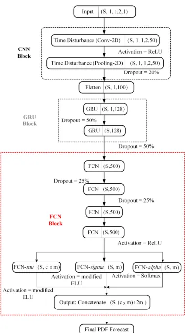
IV. PROPOSEDDEEPMIXTURENETWORKARCHITECTURE The structure of the designed deep mixture neural network is depicted in Fig.1. To associate the PDF forecasts to the look-ahead times, the residential load data corresponding to the time-lags (lag = 2 [2][11]) are selected as input dataset,xifor

the proposed PDF forecasting approach. The input set is a dimensional tensor with(S,1,1,2,1)size. The proposed end-to-end deep mixture approach consists of three main blocks, including CNN, GRU, and FCN blocks, which is described in the following subsections.

Fig. 1. Structure of designed deep mixture neural networks

A. CNN Block

In this paper, the CNN block consists of a convolution layer and a pooling layer. The convolution operator outputs feature maps by convolving the feature maps from the previous layer with filter sets. Max pooling layer is utilized to strengthen the features learned and expressed in the previous layers. This layer usually takes the maximum of the input value to create its own feature maps and is applied to each feature map independently. Max pooling layer reduces information redundancy and size to enhance computational efficiency and numerical stability. As can be seen in Fig.1, the raw input set of the convolution layer converts to (S,1,1,2,50)vectors (S stands for sample). Max pooling pools the maximum over each time interval as its output feature map and forms the features as vectors with dimension(S,1,1,2,50).

(6)

B. GRU Block

The GRU block learns short and long-term dependencies and captures temporal features. The GRU block comprises two GRU layers to allow the proposed deep mixture network to freely determine the amount of information to use in each time interval. Each GRU layer is characterized by the update gateu(m, L, t), and reset gater(m, L, t), as follows:

u(m, L, t) =f[ωuy(m, L, t)+Ruh(L, t−1)+bu(m, L)] (8) r(m, L, t) =f[ωry(m, L, t) +Rrh(L, t−1) +br(m, L)] (9) h(L, t) = (1−u(m, L, t))h(L, t−1) +u(m, L, t)∼h(L, t) (10) ∼ h(L, t) =f[ωhy(m, L, t) +Ru(r(m, L, t)h(L, t−1))] (11) where GRU parameters including allω∈Rd×k,R∈Rd×k,

and b ∈ Rd are learning weights, recurrent parameters, and

biases, respectively, shared by all time intervals and learned during training. Furthermore, k is a hyper-parameter and

denotes the element-wise product. The ReLU activation function is adopted for GRU gates, and hidden and candidate states. The update gate controls how many hidden states h(.)

must be updated, and the reset gate controls the impression of the hidden state h(.) at previous time step t−1 on the candidate state ∼h.

The outputs of the CNN block are flattened and the first GRU layer is initialized with (S,1,100). When passing through GRU layers, the input of these recurrent-based layers convert to (S,1,128) and (S,128) in the output of first and second GRU layers, respectively. Theoretically, two GRU layers are sufficient to handle highly fluctuating time series, such as small-scale solar generation [19]. Furthermore, after experimenting with more layers, we concluded that increasing the number of GRU layer does not bring any performance improvement. Afterwards, the output of these two layers are regularized via dropout with 50% probability. Dropout is carried out to prevent overfitting and reduces the information required for training of the deep mixture network [48]. C. FCN Block

The deep mixture network ends with several FCN layers, making up the FCN block. Selecting the FCN layers is highly sensitive, since striking a balance between maximum usage capability in the learning process and preventing overfitting, degradation, and gradient vanishing are challenging and re-quire comprehensive trial and error. In the end, we selected four FCN layers. In addition, to control the dimension of the GRU, the first four FCNs are trained end-to-end to enhance the performance without further machinery [49], while to prevent overfitting two FCN layers are dropped out with 25% probability. The next three FCNs construct the coefficient of the modified MDN. FCN-alpha, FCN-sigma, and FCN-mu approximateαn(x, t),σn(x, t), andµn(x, t) in a parallelized

manner. In the final step, the approximated parameters to forecast PDF based on (1) are concatenated.

V. RESULTS ANDDISCUSSION

For our experiments, we used real smart meter household load data of London city, collected between 1 February 2012 to 1 February 2013 , for 5567 houses sampled at 30-minute resolution [50]. The input data is load power consumption of the residential loads and corresponding meteorological data i.e. temperature, humidity, solar irradiance, and wind speed. Furthermore, to validate the proposed method structure, we consider a single residential load dataset within 1-min resolu-tion (available online at [51]) as an extreme PRLF problem. This dataset comprises a household with five family members over the period of 1 June 2012 to 30 June 2012. To eval-uate different methods, we implemented the proposed PRLF methods and other methods in a rolling approach and used fixed windows of data to train parameters and tested based on the out-of-sample data. 70% of the dataset is dedicated to training, and 30% for testing. To address the applicability of the proposed methodology for load forecasting, three different cases are discussed, i) A single residential customer targeting smart house scheduling, ii) 121 residential customers targeting residential microgrids, and iii) 3516 household load data are aggregated, targeting distribution system operators decision making. All the forecasting methods are implemented in the TensorFlow package in a PC with Intel Core i7-5960X CPU@ 3.00 GHz, 32-GB RAM memory.

Mean absolute percentage error (MAPE) and root mean square error (RMSE), as used in [40] for load forecasting using deep learning networks, are used as performance metrics:

RM SE= v u u u t N P t=1 (yre−yf)2 N (12) M AP E = N P t=1 |yre−yf yre | N (13)

where yre is the real value, yf is the forecast value, and

N is the number of yf. Furthermore, to evaluate the PDF

forecasting comprehensively, two additional metrics are used. The continuous ranked probability score (CRPS) assesses the calibration and sharpness of the forecasted PDF simultane-ously, as [52] : CP RSt= 1 N N X i=1 1 Z 0 CDF(yf(t))−CDF(yre(t))dy (14)

whereCDF(yf(t))/CDF(yre(t))is the predictive/real

cu-mulative distribution function [31]. Cross-entropy (CE) is an-other metric that is utilized in this paper for PRLF assessment, which is defined as:

CE=−

N X

i=1

p(Y|X) log (p(Y|X)) (15) CE is more sensitive to rare events than CRPS. If the mea-sured load values are very different to the mean value of load, with CRPS, PRLF method results are very good. However, with CE, if this perturbation is out of the distribution, CE shows that the PRLF method has infinite error. The general

(7)

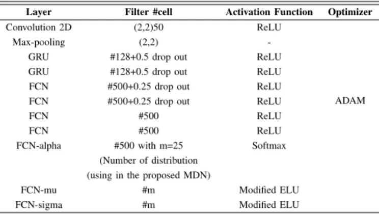
framework of the proposed deep mixture density network with CNN, GRU, and fully-connected layers is given in Table II. The proposed deep mixture density network involves the 2D-CNN with 950 epochs and two GRUs with 128 units. Note that mshows the number of the distribution, which is used in the proposed deep mixture density network.

TABLE II

PARAMETERS OF THE PROPOSED DEEP MIXTURE DENSITY NETWORK

Layer Filter #cell Activation Function Optimizer

Convolution 2D (2,2)50 ReLU

ADAM

Max-pooling (2,2)

-GRU #128+0.5 drop out ReLU GRU #128+0.5 drop out ReLU FCN #500+0.25 drop out ReLU FCN #500+0.25 drop out ReLU

FCN #500 ReLU

FCN-alpha #500 with m=25 Softmax (Number of distribution

(using in the proposed MDN)

FCN-mu #m Modified ELU

FCN-sigma #m Modified ELU

For the sake of comparison, some state-of-the-art PRLF models are applied to construct PDF with the same dataset including 2D-CNN, GRU, and LSTM as deep structure-based forecasting models, and random forest (RF) and feedforward neural network (FFNN) as shallow based forecasting models to verify the CNN-GRU performance. Firstly, state-of-the-art structures, which are integrated into the proposed MDN are:

• 2D-CNN with 950 epochs, (2,2)50 (filter), including two convolutional layers and four FCN layers with ReLU activation function.

• GRU is utilized with 1000 epochs, 128 units, two GRU and four FCN layers, and the ReLU activation function. • LSTM is implemented with ReLU activation function, 1000 epochs and 128 units, with two LSTM and four FCN layers.

• RF is merged into the proposed MDN with 350 trees. • FFNN integrated into the proposed MDN with 1024

epochs, one input layer, two hidden layers, one output layers and 500 cells.

Furthermore, the proposed deep mixture method is com-pared with the Monte-Carlo dropout technique and kernel density estimator (KDE) to demonstrate the superiority of the proposed method in reconstructing PDF. Furthermore, the combined probabilistic load forecasting method CPRLF of [39] is also considered for benchmarking. CRPLF comprises of three Gaussian process regression (GPR) and four neural network layers, using CRPS as loss function and optimized as a quadratic problem. The detailed parameters of the CRPLF are given in [39].

A. Case I

In this subsection, the performance of the proposed deep mixture for the PDF prediction of a single household load, as the most fluctuating load, is examined.

Fig. 2. CNN-GRU mixture predictive distribution and actual values at a sample day (a) 00:00, (b) 8:30, (c) 13:00, (d) 20:30 in Case I

Fig. 3. PIs with different confidence intervals obtained by proposed deep mixture model in Case I

Predicted PDF for various hours of a day and the as-sociated real values obtained by the designed CNN-GRU mixture network are shown in Fig.2. Figs 2(a) and 2(c) shows individual PDFs for off-peak (00:00) and mid-peak (08:30) hours, respectively. In addition, peak hours individual PDFs are shown in Figs 2(b) and 2(d). The real recorded residential load values are also depicted in Fig.2, in order to verify the closeness of the PDFs predicted by the proposed deep mixture. Furthermore, the sharpness of predicted PDF is clear in Fig.2. To explicitly demonstrate the performance, the prediction intervals with look-ahead time up to 48-time intervals obtained by the proposed CNN-GRU mixture network approach and actual observations in a sample day (January 29, 2012), are depicted in Fig.3, where the confidence covers the range of 10%-80%. Fig.3 shows that the designed CNN-GRU mixture network can cover the observation in constructed PIs. The

(8)

sophisticated PIs are highly variable with time, unlike the consistency of the proposed deep mixture model with highly variable household load behavior.

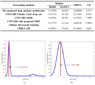
Table III compares different data-driven methods, and we can observe that the proposed CNN-GRU mixture network significantly outperforms 2D-CNN, GRU, LSTM, RF, and FFNN. For instance, RMSE of CNN-GRU is 0.1592, while RMSE of the GRU and LSTM are 0.22541 and 0.22611, respectively. The mixture CNN-GRU improves the accuracy of GRU by more than 29.23% and enhances the LSTM mixture network median accuracy by more than 29.58%. In addition, the RMSE and MAPE values of RF and FFNN show that the CNN-GRU improves the accuracy of median prediction by more than 56.02 % and 58.28% in terms of MAPE, respectively and the proposed CNN-GRU MDN enhances the accuracy of RF and FFNN close to 47.55% and 58.15% in terms of RMSE. From the results in Table I, the CRPS values show the superiority of the CNN-GRU mixture in predicting the whole distribution. The CRPS values obtained by different deep mixture load forecasting methods designed in this paper indicate that CNN-GRU improves the accuracy of predicted PDFs by more than 18.63%, 24.13%, 34.25% for 2D-CNN, GRU, and LSTM, respectively. Besides, the CE metrics confirms the previous analyses based on RMSE, MAPE, and CRPS metrics. The comparative results in terms of all four metrics values indicate that among all short-term forecasting models based MDN structures, FFNN mixture networks performs worst due to its shallow nature. The proposed deep mixture network significantly improves the predictive performance over the presented shallow mixture network by 47.77% based on CRPS. Furthermore, Table IV compares three state-of-the-art and the CPRLF method of [39]. In the state-of-the-art methods CNN-GRU is integrated into the proposed MDN without adversarial training, Monte Carlo drop out, and KDE. The CNN-GRU method exhibits the highest overall accuracy, whereas the proposed MDN without adversarial training is slightly inferior to the Monte- Carlo drop out and KDE. In addition, the proposed deep mixture structure has improved the accuracy of the CRPLF by more than 63.95% and 49.78% in terms of MAPE and CRPS values, respectively.

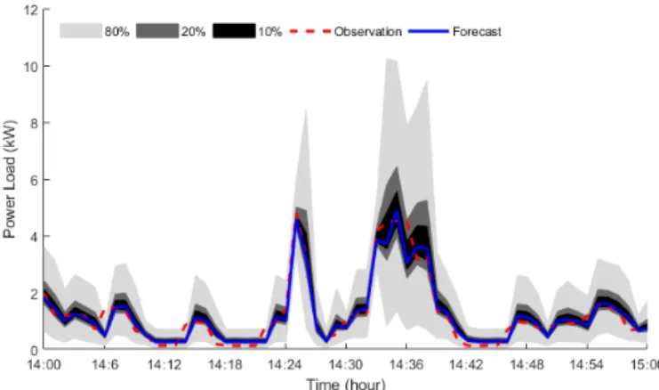
A single residential load with high level of accuracy and extremely small time resolution case can be considered as one of the most challenging time series forecasting problem in the power system. Therefore, the results obtained by the proposed deep mixture network in 1-min time resolution is also discussed. Figs. 4(a) and 4(b) show the forecasted PDF for two different time intervals at 14:06 and 15:42, respectively, indicating that the real-value appears in the forecasted PDFs with high probability. Fig. 5 illustrates PIs derived from the forecasted PDFs of a single residential load within 1-min time resolution for 60 time intervals between 14:00 and 15:00 in the sample day, with confidence in the range 80%-10%, showing that the forecasted intervals can properly cover the observations. Fig. 5 shows how the proposed deep mixture density network reacts to the high intermittency in a single residential load with 1-min time resolution.

The results obtained by different mixture density networks

including deep and shallow based models are given in Table V. The superiority of the proposed deep mixture density network is significant. As an example, in terms of CRPS, the CNN-GRU mixture network improves the accuracy of the other state-of-the-art deep mixture networks including 2D-CNN, GRU, and LSTM based mixture density networks by about 27.14%, 55.91%, and 64.96%, respectively. In comparison with shallow-based mixture density networks, the proposed method improves the accuracy of RF-based network by over 79.35% and 80.03% in terms of CRPS and CE, respectively. Also, the proposed deep mixture architecture shows more than 82% improvement in comparison with FFNN in terms of all four metrics.

Furthermore, the comparison between the proposed deep mixture density network and Monte-Carlo drop out, KDE, and CRPL is given in Table VI. The results obtained by the proposed probabilistic deep network show more than 63.05% and 74.50% in comparison with the state-of-the-art methods and Monte-Carlo drop out and the KDE, respectively. In addition, the proposed method outperforms CPRLF with 80.93% and 80.55% in terms of CE and CRPS, respectively.

TABLE III

PERFORMANCE OFFORECASTINGMETHODS FOR ASINGLEHOUSEHOLD LOAD

Forecasting methods Median CRPS% CE

RMSE MAPE%

The proposed deep mixture architecture 0.15952 10.024 0.08490 5.257

2D-CNN+The proposed MDN 0.16153 10.124 0.10435 5.952 GRU+The proposed MDN 0.22541 18.591 0.11191 6.089 LSTM+The proposed MDN 0.22611 18.8534 0.12913 6.447 RF+The proposed MDN 0.30357 22.7922 0.11592 8.655 FFNN+The proposed MDN 0.3812 24.032 0.16258 9.306 TABLE IV

PERFORMANCE OFPDF METHODS FOR ASINGLEHOUSEHOLDLOAD

RMSE MAPE%

CNN-GRU+Monte Carlo drop out 0.21153 16.124 0.11435 6.952

CNN-GRU+KDE 0.25541 18.591 0.12191 7.089

CNN-GRU+the proposed MDN

0.17715 12.136 0.09120 5.9851

without adversarial training

CPRLF [39] 0.39913 27.814 0.16905 9.627

(a) (b)

Fig. 4. CNN-GRU mixture predictive distribution and actual values at a sample day with 1-min time resolution (a) 14:06, (b) 15:42 in Case I

(9)

Fig. 5. PIs with different confidence intervals obtained by proposed deep mixture model with 1-min time resolution in Case I

TABLE V

PERFORMANCE OF FORECASTING METHODS FOR A SINGLE HOUSEHOLD LOAD WITHIN 1-MIN RESOLUTION

RMSE MAPE%

2D-CNN+The proposed MDN 0.02914 13.1270 0.029531 1.1495 GRU+The proposed MDN 0.07215 19.9134 0.048803 2.0598 LSTM+The proposed MDN 0.07392 21.6324 0.061419 2.3357 RF+The proposed MDN 0.11176 28.0975 0.104218 5.6787 FFNN+The proposed MDN 0.15318 32.2785 0.384916 6.9058 B. Case II

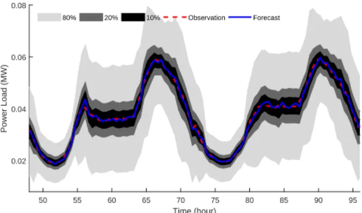
In this case, PRLF is carried out for a typical low voltage microgrid that consists of 121 residential loads. Fig. 6 depicts the predicted PDFs by designed deep mixture network and corresponding real values. These figures provide a sample set of forecasting PDFs, with full probability description of a set of small-scale aggregative loads. Almost all real values placed in the middle of PDF curves demonstrate the high accuracy of the proposed network and its practical applications in short/long term planning of residential microgrids.

To show the performance of the proposed neural network in capturing the inherent uncertainty and nonstationarity asso-ciated with household loads, Fig.7 shows the forecasted PIs with different confidence intervals for 48 hours. In the Fig.7, real residential load values are always placed in the PIs and actual values trajectories are tracked using the constructed PIs. Table VII is intended to demonstrate the superiority of the designed CNN-GRU mixture with respect to the other designed mixture networks. This table shows that the disaggre-gated loads are more fluctuating than aggredisaggre-gated loads, even with aggregated loads with small-scale level. Secondly, CNN-GRU mixture outperforms the rest of the designed mixture neural networks. As an example, CNN-GRU mixture has improved the 2D-CNN, GRU, LSTM, RF and FFNN mixture accuracy by more than 17.09%, 43.54%, 49.88%, 59.78% and 64.23%, respectively, based on the CE metric.

In addition, the proposed approach is compared with GRU + the proposed MDN without adversarial training, CNN-GRU+ Monte-Carlo drop out, CNN-CNN-GRU+KDE, and CRPLF in Table VIII. The proposed PRLF method is more accurate

TABLE VI

PERFORMANCE OF PDF METHODS FOR A SINGLE HOUSEHOLD LOAD WITHIN 1-MIN RESOLUTION

RMSE MAPE%

CNN-GRU+KDE 0.15623 23.0462 0.084387 4.7655

0.03604 15.2547 0.036425 1.8942

CPRLF [39] 0.18479 28.6278 0.110656 5.9463

Fig. 6. CNN-GRU mixture predictive distribution and actual values at a sample day for (a) 00:00, (b) 8:30, (c) 13:00, (d) 20:30 in Case II

than the proposed MDN without adversarial training, Monte-Carlo drop out, KDE, and CPRLF methods and improves the accuracy of the proposed MDN without adversarial training, Monte-Carlo drop out, and KDE by more than 39.53%, 53.35%, 60.56%, and 66.94%, respectively, in terms of CE.

C. Case III

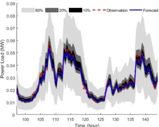
3516 residential loads are aggregated to form set of large-scale residential loads. The predicted PDFs for several hours-ahead of a sample day is depicted in Fig.8. In peak (Figs 8 (c) and (d)) mid-peak (Fig.8 (b)), and off-peak hours (Fig 8(a)) the results display great accuracy in aggregated loads at megawatt level. The predicted PDF for look-ahead hours can provide full statistical information for retail and wholesale market participants and distribution or transmission system operators with a high level of accuracy, which is demonstrated by inserting real values in the middle of the PDF. Furthermore, anticipated PIs in this case are shown in Fig.9, which we see that real values lie in middle of PDFs. The superiority of the proposed deep mixture network in comparison with state-of-the-art and previous presented method is verified by results in Tables IX & X.

(10)

50 55 60 65 70 75 80 85 90 95 Time (hour) 0.02 0.04 0.06 0.08 Power Load (MW) 80% 20% 10% Observation Forecast

Fig. 7. PIs with different confidence intervals obtained by proposed deep mixture model in Case II

TABLE VII

PERFORMANCE OFFORECASTINGMETHODS FOR ASET OF SMALL-SCALEAGGREGATIVERESIDENTIALLOAD

RMSE MAPE%

2D-CNN+The proposed MDN 0.003077 6.7697 0.005160 2.8985 GRU+The proposed MDN 0.004480 11.9473 0.006562 4.2563 LSTM+The proposed MDN 0.004547 11.9823 0.007001 4.7952 RF+The proposed MDN 0.127431 18.8491 0.014193 5.9757 FFNN+The proposed MDN 0.290020 20.0456 0.026876 6.1654 VI. CONCLUSION

In this paper, a direct PRLF model based on deep mixture networks was proposed. The proposed model is capable of capturing the uncertainty of a single household load as well as small/large scale aggregated loads. First, the mixture density network is reformulated to mitigate the limitations of its stan-dard form in terms of NaN values of variance by integrating the log-sum-exp trick and adversarial training. Then, an end-to-end deep mixture network exploits the strengths of CNN to extract feature maps, GRU to capture temporal features, and concatenated FCN to construct proposed MDN coefficients to forecast PDF. To verify the performance of the proposed method, three cases based on the aggregated/disaggregated loads with 1-min (as an extreme PRLF problem) and 30-min time resolutions are studied in this paper. The state-of-the-art deep- and shallow-based models are designed for the sake of comparison with the proposed neural network model. The obtained results show more than 20% improvement in accuracy compared to deep structure-based methods and more than 60% accuracy improvement in comparison with RF and FFNN mixture network. Furthermore, the designed CNN-GRU method is merged into the proposed MDN without adversarial training and Monte-Carlo dropout methods to address the superiority of the proposed predictive PDF estimators. The results shows more than 25% accuracy improvement. In addi-tion, the results obtained by the proposed deep mixture density network is also compared with the CRPLF method and shows at least 47% improvement in terms of all accuracy metrics. The obtained results show the great achievement of the proposed method in probabilistic forecasting of the residential loads

TABLE VIII

PERFORMANCE OFPDF METHODS FOR ASET OFSMALL-SCALE AGGREGATIVERESIDENTIALLOAD

RMSE MAPE%

CNN-GRU+KDE 0.02980 12.254 0.02119 6.094

0.005740 9.2547 0.00569 3.9746

CPRLF [39] 0.11576 21.632 0.02797 7.268

Fig. 8. CNN-GRU mixture predictive distribution and actual values at a sample day for (a) 00:00, (b) 8:30, (c) 13:00, (d) 20:30 in Case III

from a single customer to large-scale aggregated loads, which can be implemented as separate modules to be embedded smart buildings/ microgrid control centers/ distribution system control centers.

ACKNOWLEDGMENT

This work was partly supported by the European Com-mission under the ’H2020-EU.3.3.1- Reducing energy con-sumption and carbon footprint by smart and sustainable use’ program topic, according to the Grant Agreement No. 767625.

REFERENCES

[1] M. Rastegar, “Impacts of residential energy management on reliability of distribution systems considering a customer satisfaction model,” IEEE Transactions on Power Systems, vol. 33, no. 6, pp. 6062–6073, Nov 2018.

[2] W. Kong, Z. Y. Dong, D. J. Hill, F. Luo, and Y. Xu, “Short-term residential load forecasting based on resident behaviour learning,”IEEE Transactions on Power Systems, vol. 33, no. 1, pp. 1087–1088, Jan 2018. [3] H. Shi, M. Xu, and R. Li, “Deep learning for household load forecastinga novel pooling deep rnn,”IEEE Transactions on Smart Grid, vol. 9, no. 5, pp. 5271–5280, Sept 2018.

[4] Y. Wang, N. Zhang, Y. Tan, T. Hong, D. S. Kirschen, and C. Kang, “Combining probabilistic load forecasts,”IEEE Transactions on Smart Grid, pp. 1–1, 2018.

(11)

Fig. 9. PIs with different confidence intervals obtained by proposed deep mixture model in Case III

TABLE IX

PERFORMANCE OFFORECASTINGMETHODS FOR ASET OF LARGE-SCALEAGGREGATIVERESIDENTIALLOAD

RMSE MAPE%

2D-CNN+The proposed MDN 0.02474 1.52936 0.044170 5.9584

GRU+The proposed MDN 0.033122 2.51983 0.078941 6.2548

LSTM+The proposed MDN 0.032267 2.33757 0.062364 6.3600

RF+ The proposed MDN 0.05281 5.34392 0.12655 8.1712

FFNN+The proposed MDN 0.05001 5.50106 0.132456 8.2563

[6] H. Zen and A. Senior, “Deep mixture density networks for acoustic modeling in statistical parametric speech synthesis,” in 2014 IEEE International Conference on Acoustics, Speech and Signal Processing (ICASSP), May 2014, pp. 3844–3848.

[7] M. Khodayar, O. Kaynak, and M. E. Khodayar, “Rough deep neural architecture for short-term wind speed forecasting,”IEEE Transactions on Industrial Informatics, vol. 13, no. 6, pp. 2770–2779, Dec 2017. [8] N. Mohan, K. Soman, and S. S. Kumar, “A data-driven strategy for

short-term electric load forecasting using dynamic mode decomposition model,”Applied Energy, vol. 232, pp. 229 – 244, 2018.

[9] K. G. Boroojeni, M. H. Amini, S. Bahrami, S. Iyengar, A. I. Sarwat, and O. Karabasoglu, “A novel multi-time-scale modeling for electric power demand forecasting: From short-term to medium-term horizon,”Electric Power Systems Research, vol. 142, pp. 58 – 73, 2017.

[10] C. Bikcora, L. Verheijen, and S. Weiland, “Density forecasting of daily electricity demand with arma-garch, caviar, and care econometric models,”Sustainable Energy, Grids and Networks, vol. 13, pp. 148 – 156, 2018.

[11] Z. Shi, H. Liang, and V. Dinavahi, “Direct interval forecast of uncertain wind power based on recurrent neural networks,”IEEE Transactions on Sustainable Energy, vol. 9, no. 3, pp. 1177–1187, July 2018. [12] G. J. Tsekouras, N. D. Hatziargyriou, and E. N. Dialynas, “An optimized

adaptive neural network for annual midterm energy forecasting,”IEEE Transactions on Power Systems, vol. 21, no. 1, pp. 385–391, Feb 2006. [13] Y. Wang, Q. Xia, and C. Kang, “Secondary forecasting based on deviation analysis for short-term load forecasting,”IEEE Transactions on Power Systems, vol. 26, no. 2, pp. 500–507, May 2011.

[14] A. Lahouar and J. B. H. Slama, “Day-ahead load forecast using random forest and expert input selection,”Energy Conversion and Management, vol. 103, pp. 1040 – 1051, 2015.

[15] Y. Chen, P. B. Luh, C. Guan, Y. Zhao, L. D. Michel, M. A. Coolbeth, P. B. Friedland, and S. J. Rourke, “Short-term load forecasting: Similar day-based wavelet neural networks,” IEEE Transactions on Power Systems, vol. 25, no. 1, pp. 322–330, Feb 2010.

[16] S. Li, P. Wang, and L. Goel, “A novel wavelet-based ensemble method for short-term load forecasting with hybrid neural networks and feature

TABLE X

PERFORMANCE OFPDF METHODS FOR ASET OFLARGE-SCALE AGGREGATEDRESIDENTIALLOADS

RMSE MAPE%

CNN-GRU+KDE 0.2254 8.649 0.11342 6.025

0.06525 3.2541 0.0754 5.5136

CPRLF [39] 0.09421 7.485 0.12280 8.814

selection,” IEEE Transactions on Power Systems, vol. 31, no. 3, pp. 1788–1798, May 2016.

[17] S. Afrasiabi, M. Afrasiabi, B. Parang, and M. Mohammadi, “Integration of accelerated deep neural network into power transformer differential protection,”IEEE Transactions on Industrial Informatics, pp. 1–1, 2019. [18] M. Q. Raza, M. Nadarajah, J. Li, and K. Y. Lee, “Multivariate ensemble forecast framework for demand prediction of anomalous days,” IEEE Transactions on Sustainable Energy, pp. 1–1, 2018.

[19] M. Ravanelli, P. Brakel, M. Omologo, and Y. Bengio, “Light gated recurrent units for speech recognition,”IEEE Transactions on Emerging Topics in Computational Intelligence, vol. 2, no. 2, pp. 92–102, 2018. [20] S. Lai, L. Xu, K. Liu, and J. Zhao, “Recurrent convolutional neural

networks for text classification.” inAAAI, vol. 333, 2015, pp. 2267– 2273.

[21] W. Zhang, H. Quan, and D. Srinivasan, “An improved quantile regression neural network for probabilistic load forecasting,”IEEE Transactions on Smart Grid, pp. 1–1, 2018.

[22] D. Sez, F. vila, D. Olivares, C. Caizares, and L. Marn, “Fuzzy prediction interval models for forecasting renewable resources and loads in micro-grids,” IEEE Transactions on Smart Grid, vol. 6, no. 2, pp. 548–556, March 2015.

[23] M. A. Hosen, A. Khosravi, S. Nahavandi, and D. Creighton, “Improving the quality of prediction intervals through optimal aggregation,” IEEE Transactions on Industrial Electronics, vol. 62, no. 7, pp. 4420–4429, July 2015.

[24] Y. Wang, Z. Zhou, A. Botterud, and K. Zhang, “Optimal wind power uncertainty intervals for electricity market operation,”IEEE Transactions on Sustainable Energy, vol. 9, no. 1, pp. 199–210, Jan 2018. [25] R. Li and Y. Jin, “A wind speed interval prediction system based

on multi-objective optimization for machine learning method,”Applied Energy, vol. 228, pp. 2207 – 2220, 2018.

[26] Z. Men, E. Yee, F.-S. Lien, D. Wen, and Y. Chen, “Short-term wind speed and power forecasting using an ensemble of mixture density neural networks,”Renewable Energy, vol. 87, pp. 203 – 211, 2016.

[27] S. B. Taieb, J. W. Taylor, and R. J. Hyndman, “Hierarchical proba-bilistic forecasting of electricity demand with smart meter data,”URL: https://robjhyndman.com/papers/HPFelectricity.pdf, 2017.

[28] L. Alfieri and P. De Falco, “Wavelet-based decompositions in proba-bilistic load forecasting,”IEEE Transactions on Smart Grid, pp. 1–1, 2019.

[29] C. Feng, M. Sun, and J. Zhang, “Reinforced deterministic and proba-bilistic load forecasting via q-learning dynamic model selection,”IEEE Transactions on Smart Grid, pp. 1–1, 2019.

[30] S. Haben, G. Giasemidis, F. Ziel, and S. Arora, “Short term load forecasting and the effect of temperature at the low voltage level,”

International Journal of Forecasting, vol. 35, no. 4, pp. 1469–1484, 2019.

[31] Y. Wang, D. Gan, M. Sun, N. Zhang, Z. Lu, and C. Kang, “Probabilistic individual load forecasting using pinball loss guided lstm,” Applied Energy, vol. 235, pp. 10 – 20, 2019.

[32] A. Elvers, M. Vo, and S. Albayrak, “Short-term probabilistic load fore-casting at low aggregation levels using convolutional neural networks,” in2019 IEEE Milan PowerTech, 2019, pp. 1–6.

[33] W. Xie, P. Zhang, R. Chen, and Z. Zhou, “A nonparametric bayesian framework for short-term wind power probabilistic forecast,” IEEE Transactions on Power Systems, pp. 1–1, 2018.

[34] S. Chai, Z. Xu, and Y. Jia, “Conditional density forecast of electricity price based on ensemble elm and logistic emos,”IEEE Transactions on Smart Grid, pp. 1–1, 2018.

(12)

[35] T. Hong and S. Fan, “Probabilistic electric load forecasting: A tutorial review,”International Journal of Forecasting, vol. 32, no. 3, pp. 914– 938, 2016.

[36] T. Hong, P. Pinson, S. Fan, H. Zareipour, A. Troccoli, and R. Hyndman, “Probabilistic energy forecasting: Global energy forecasting competition 2014 and beyond,”International Journal of Forecasting, vol. 32, no. 3, pp. 896–913, 2016.

[37] S. Arora and J. W. Taylor, “Forecasting electricity smart meter data using conditional kernel density estimation,”Omega, vol. 59, pp. 47–59, 2016. [38] K. Chen, K. Chen, Q. Wang, Z. He, J. Hu, and J. He, “Short-term load forecasting with deep residual networks,”IEEE Transactions on Smart Grid, pp. 1–1, 2018.

[39] T. Li, Y. Wang, and N. Zhang, “Combining probability density forecasts for power electrical loads,”IEEE Transactions on Smart Grid, pp. 1–1, 2019.

[40] W. Kong, Z. Y. Dong, Y. Jia, D. J. Hill, Y. Xu, and Y. Zhang, “Short-term residential load forecasting based on lstm recurrent neural network,”

IEEE Transactions on Smart Grid, vol. 10, no. 1, pp. 841–851, Jan 2019.

[41] A. Kavousi-Fard, A. Khosravi, and S. Nahavandi, “A new fuzzy-based combined prediction interval for wind power forecasting,”IEEE Transactions on Power Systems, vol. 31, no. 1, pp. 18–26, Jan 2016. [42] C. Robert, “Machine learning, a probabilistic perspective,” CHANCE,

vol. 27, no. 2, pp. 62–63, 2014.

[43] A. Kurakin, I. Goodfellow, and S. Bengio, “Adversarial machine learning at scale,”arXiv preprint arXiv:1611.01236, 2016.

[44] A. Nøkland, “Improving back-propagation by adding an adversarial gradient,”arXiv preprint arXiv:1510.04189, 2015.

[45] D. P. Kingma and J. Ba, “Adam: A method for stochastic optimization,”

arXiv preprint arXiv:1412.6980, 2014.

[46] A. L. Maas, A. Y. Hannun, and A. Y. Ng, “Rectifier nonlinearities improve neural network acoustic models,” in in ICML Workshop on Deep Learning for Audio, Speech and Language Processing. Citeseer, 2013.

[47] D.-A. Clevert, T. Unterthiner, and S. Hochreiter, “Fast and accurate deep network learning by exponential linear units (elus),”arXiv preprint arXiv:1511.07289, 2015.

[48] N. Srivastava, G. Hinton, A. Krizhevsky, I. Sutskever, and R. Salakhut-dinov, “Dropout: a simple way to prevent neural networks from over-fitting,”The Journal of Machine Learning Research, vol. 15, no. 1, pp. 1929–1958, 2014.

[49] J. Long, E. Shelhamer, and T. Darrell, “Fully convolutional networks for semantic segmentation,” inThe IEEE Conference on Computer Vision and Pattern Recognition (CVPR), 2015.

[50] London datastore. [Online]. Available: https://data.london.gov.uk [51] IEEE Power-Energy Society (PES) open dataset. [Online]. Available:

https://site.ieee.org/pes-iss/data-sets

[52] Y. Lin, M. Yang, C. Wan, J. Wang, and Y. Song, “A multi-model combination approach for probabilistic wind power forecasting,”IEEE Transactions on Sustainable Energy, vol. 10, no. 1, pp. 226–237, Jan 2019.