Scholarship@Western
Scholarship@Western
Electronic Thesis and Dissertation Repository
10-1-2018 10:30 AM
Development Of Material Model Subroutines For Linear And
Development Of Material Model Subroutines For Linear And
Nonlinear Response Of Elastomers
Nonlinear Response Of Elastomers
Asim Gillani
The University of Western Ontario
Supervisor Liying Jiang
The University of Western Ontario Co-Supervisor Samuel Asokanthan
The University of Western Ontario
Graduate Program in Mechanical and Materials Engineering
A thesis submitted in partial fulfillment of the requirements for the degree in Master of Engineering Science
© Asim Gillani 2018
Follow this and additional works at: https://ir.lib.uwo.ca/etd
Part of the Applied Mechanics Commons
Recommended Citation Recommended Citation
Gillani, Asim, "Development Of Material Model Subroutines For Linear And Nonlinear Response Of Elastomers" (2018). Electronic Thesis and Dissertation Repository. 5837.
https://ir.lib.uwo.ca/etd/5837
This Dissertation/Thesis is brought to you for free and open access by Scholarship@Western. It has been accepted for inclusion in Electronic Thesis and Dissertation Repository by an authorized administrator of
The nature of elastomers has been extensively studied ever since the vulcanization of rubber in the
19th century. Elastomers have been heavily employed in various fields, such as automobile,
aerospace, robotics, biomimetics, dynamics and energy harvesting. Due to their molecular nature,
these materials display hyperelastic and viscous response when deformed. Their response has been
studied in a number of works, which tend to explain their nature through the theory of polymer
dynamics or using rheological models. As elastomers are designed as actuators, generators or
artificial tissues with complex geometries, the need for finite element analysis to study their
response is becoming more essential. The purpose of this study is to develop user defined
subroutines (UMATs) to capture the viscoelastic and hyperelastic response of elastomeric
materials in ABAQUS CAE. Two UMATs have been formulated based on the existing theory of
linear viscoelasticity and hyperelasticity. The developed UMATs are then tested using ABAQUS
CAE software on their accuracy, robustness and versatility. The UMAT for predicting the linear
response of elastomers can capture the time and rate-dependent response of material. However, it
showed some offset from experimental results since the material is nonlinear in nature. The UMAT
for predicting the nonlinear behavior of elastomers quite accurately capture the hyperelastic
response of the material.
Keywords
Elastomers, viscoelasticity, hyperelasticity, user material subroutine (UMAT), finite element
[iii]
Abstract ... ii
Table of Contents ... iii
List of Tables ... v
List of Figures ... vi
List of Appendices ... viii
CHAPTER 1 ... 1
1
Introduction ... 1
1.1
Elastomers ... 1
1.2
Characteristics of elastomers ... 2
1.3
Applications of elastomers ... 3
1.4
Objectives ... 5
1.5
Thesis Structure ... 6
CHAPTER 2 ... 7
2
Literature review on fundamental material models for elastomers ... 7
2.1
Hyperelastic models for elastomeric materials ... 7
2.2
Viscoelastic models for elastomeric materials ... 12
2.2.1
Element under a simple strain………..13
2.2.2
Rheological models………..16
2.2.3
Modeling of viscoelastic elastomers……….21
CHAPTER 3 ... 24
3.1.1
Stress and strain………24
3.1.2
Boltzmann superposition principle………...25
3.2
Numerical formulation for linear response of elastomers... 25
3.3
Development of UMAT for linear viscoelastic response ... 32
3.3.1
Formulation of UMAT for linear viscoelastic analysis………....32
3.4
Testing with ABAQUS ... 37
3.5
Summary ... 47
CHAPTER 4 ... 48
4
Finite element modeling of nonlinear response of elastomers ... 48
4.1
Constitutive equations for materials under large deformations ... 48
4.1.1
Equation of stresses for nonlinear response……….48
4.2
Development of UMAT for nonlinear hyperelastic response ... 50
4.3
Testing with ABAQUS ... 54
4.4
Summary ... 61
CHAPTER 5 ... 62
5
Conclusion and future working ... 62
5.1
Conclusion ... 62
5.2
Future work ... 63
APPENDIX ... 64
Appendix. Basic Definitions for terms used in UMAT ... 64
[v]
List of Tables
Table 3-1 Parameters for VHB 4910 obtained after parametric study ... 42
Table 3-2 Convergence test data for linear viscoelastic UMAT. ... 46
Table 4-1 Material parameters for testing ... 55
Figure 2-1 An element under a simple shear strain ... 13
Figure 2-2 Relaxation test for a viscoelastic material [10]. ... 15
Figure 2-3 Creep test for a viscoelastic material [10]. ... 16
Figure 2-4 The spring and damper elements. ... 17
Figure 2-5 The Maxwell element. ... 18
Figure 2-6 The Kelvin-Voigt model. ... 19
Figure 2-7 (a) Generalized Maxwell model; (b) Generalized Kelvin model. ... 20
Figure 2-8 The Zener model. ... 20
Figure 3-1
Relaxation test of a Maxwell element [70] ... 26
Figure 3-2 Generalized Maxwell rheological model with N Maxwell chains. ... 28
Figure 3-3 A unit element under simple tension. ... 38
Figure 3-4 Deformed configuration of a unit element under tension. ... 38
Figure 3-5 A unit element under a simple shear. ... 39
Figure 3-6 Deformed configuration of a unit element under a simple shear. ... 39
Figure 3-7 Comparison of stress-strain for ABAQUS simulation and analytical calculation for
tensile test... 40
Figure 3-8 Comparison of stress-strain for ABAQUS simulation and analytical calculation for
shear test... 41
[vii]
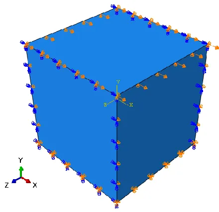
Figure 3-11 Complex geometry configuration of a specimen. ... 44
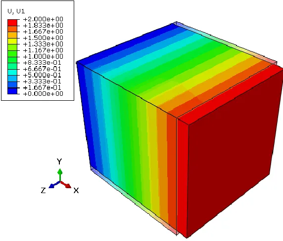
Figure 3-12 Displacement profile at time t=9 seconds. ... 44
Figure 3-13 Von Mises stress at time t=9 seconds. ... 45
Figure 3-14 Reaction force vs displacement under a cyclic loading for VHB 4910. ... 45
Figure 3-15 Variation of principal stress in y-direction with number of elements. ... 46
Figure 3-16 Variation of maximum von Mises stress with number of elements. ... 47
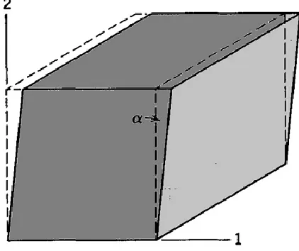
Figure 4-1 Uniaxial deformation of single element. ... 56
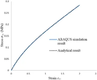
Figure 4-2 Comparison of analytical and FE results from ABAQUS for simple tension. ... 57
Figure 4-3 Simple shear for single element. ... 58
Figure 4-4 Comparison of analytical results with FE results from ABAQUS for a shear test. .... 58
Figure 4-5 Comparison between experimental results for VHB4910 and ABAQUS simulation 59
Figure 4-6 Variation of principal stress in y-direction with number of elements. ... 60
Figure 4-7 Variation of maximum von Mises stress with number of elements. ... 61
Figure A-1 Flow chart for the interaction of ABAQUS and UMAT. ...
Error! Bookmark not
CHAPTER 1
1
Introduction
Ever since the discovery of vulcanization of rubber in 1893 [1] to the introduction of dielectric
elastomers at the end of the 20thth century [2], elastomers have been an important part of
research and scientific discovery. Elastomers consist of polymer networks formed by
cross-linking highly mobile and flexible polymer chains. These materials have been extensively
employed in various engineering applications such as vibration damping, automotive industry,
robotics, biomechanics, and aerospace, just to name a few [3]. Their capability of undergoing
large deformation has made their mechanics an active research area for many years [1]. The
capability of elastomers to sustain strains of over a few hundred percent and the exhibition of
nonlinear time and rate dependent response is due to their hyperelastic and viscous nature.
Hence, their mechanics has been a prime focus in the research community [4]. Substantial
efforts have been devoted to the development of rheological models to understand the
finite-deformation and viscoelastic response of these materials. Their applications in the field of
actuation and energy harvesting has made the demand of understanding the experimental
responses of elastomeric materials through computational methods a necessity. Finite element
analysis of complex geometries and complicated stress fields observed in various applications
of these materials has become the recent target of many research studies. The motivation behind
the present study stems itself from the growing demand of numerical techniques to model the
mechanical behavior of elastomeric materials and to simulate their linear and nonlinear
responses. To serve this purpose, customized material models are usually added into the
libraries of finite element simulation software like ABAQUS CAE through user-defined
subroutines called UMATs. The primary objective of this work is to formulate finite element
(FE) models to study the linear and nonlinear responses of elastomeric materials through
developing UMAT codes in ABAQUS. The FE models are further validated through available
experimental data.
1.1 Elastomers
Polymers are materials which are composed of long molecular chains of covalently bonded
atoms, with each chain being a repetition of much smaller units called monomers [5].
Most common types of elastomers include rubbers, polyurethanes (materials for making fabric
and plastics), polybutadiene (materials for making wheels or tires), neoprene (materials for
insulations and belts) and silicone [6].
Elastomers are among the most extensively used materials nowadays. With the
discovery of cutting edge electroactive materials like dielectric elastomers, their applications
in the field of robotics, biomimetics, dynamics and energy harvesting have made them
immensely popular both in academia research fields and industry [7].
1.2 Characteristics of elastomers
Almost without exception, elastomers belong to a class of polymers which are viscoelastic in
nature[8]. The strong and flexible cross-linked ground polymer networks in these materials are
the main reason for them undergoing large deformation (hyperelasticity). Whereas elastomeric
materials demonstrate a time and rate dependent response attributed to the diffusion of these
polymer chains [3]. The classical theory of linear elasticity deals with the properties of
materials which are elastic in nature, i.e., the stress-strain relation is of direct proportionality,
as per Hooke’s law [9]. On the other hand, the classical theory of hydrodynamics, deals with
the properties of viscous liquids, for which the stress is rather proportional to the strain rate
instead of the direct relation between the stress and the strain. Both these models are
idealizations for materials with infinitesimal strains[9]. Deviations from Hookean and
Newtonian behavior are observed when dealing with finite deformation, especially for
materials which can undergo substantial dimensional changes without fracturing, such as
polymeric solutions and undiluted uncross-linked polymers [10]. Viscoelastic materials
possess properties of both viscous and elastic materials, for example, when a sinusoidal
oscillating load is applied on elastomeric materials, their strain will neither be in phase as in
elastic materials, nor will be 900 out of phase as in viscous liquids, it will be somewhere in
between [10].
The viscoelastic nature of elastomers has been immensely studied and has been the
subject for research using different models, details of which will be discussed in the subsequent
chapters. In this section some important characteristics of elastomers will be discussed.
a) The predominant characteristics of elastomers is their ability of elastic recovery after
under ideal circumstances, the material will return to their original dimensions after the
removal of stress [1].
b) Elastomers have the capability to undergo large deformation, even more than 300% in
some cases [6], this is one of the main reasons they are used for a variety of actuating
or dynamic purposes;
c) Elastomers are characterized by high fracture toughness under static or dynamic
stresses and better abrasion resistance than that of some metals like steel [1].
d) Dielectric elastomers, one type of elastomers, possess electromechanical coupling
properties, which enables them for applications in transduction technology as actuators,
sensors and energy harvesters [7]. Due to their capability of sustaining large
deformation, they have applications in actuation. The efficiency of electromechanical
coupling for elastomeric materials is higher compared to some other traditional
transduction materials such as piezoelectric [11]. Materials such as silicone rubbers
have shown strains over 30%, actuation pressures of 1.3 MPa and energy densities of
0.22 J/cm3 [12] for example;
e) Some elastomers have compatible properties in terms of surface chemistry to
biomaterials, making them suitable for making artificial tissues [6];
f) Some elastomers like Rubbers are also capable of adhering to most other materials,
enabling different hybrid constructions. In combination with fibers, such as rayon,
polyamide, polyester, glass or steel-cord, the tensile strength of the hybrid is increased
considerably with a reduction in extendibility. By joining elastomers with metals,
components which combine the elasticity of elastomers with the rigidity of metals can
be achieved [1].
1.3 Applications of elastomers
Due to the characteristics described above, there is a vast multitude of applications in which
elastomers can be used. Below are just some of the generic applications of these materials to
prove how vital it is to develop an understanding of their mechanics. Rubbers are some of the
most abundantly used elastomeric materials on the planet [1]. Elastomers have excellent sealing
capability, in fact, the very first use of rubber-like materials was to form a coating over shoes
to make them water resistant [1]. Due to their effectiveness as sealants, these materials are used
as gaskets, oil pipes, steam hoses, silicone gels, and electrical cables etc. Due to their
absorbers. Elastomers are characterized by great fracture toughness under static or dynamic
stresses and by better abrasion resistance than that of steel. Due to these features, elastomers
are used in automotive parts, aerospace and industrial facilities for loading and unloading heavy
materials. It was discovered in the late 20th century that elastomers show great dielectric
capabilities. Their efficient electromechanical coupling and the capability to undergo large
deformation have attracted much attention. Even more than 500% of stretching strain[11] can
be achieved in theory. Therefore, dielectric elastomers are excellent candidates for actuators.
These actuation devices can be used in switches, robotics, electronics and various automation
devices, just to name a few. In addition to their large deformation capability, these materials
do not produce any noise as compared to mechanical actuators [13], which aids in better
acoustic control. Properties like high specific energy density [13], high speed response [14],
and good overall performance makes these materials highly desirable for use as actuators in
robotics and aero-space applications. Elastomers have also shown promise in harvesting energy
from a variety of sources such as ocean waves, wind, water currents and human motion [15].
Due to their high energy density and conversion efficiency, these materials can be used as
robust and simple “direct drive” generators [16]. Several types of energy harvesters which use
dielectric elastomers have been tested bearing positive results. One such type of energy
harvesters is buoy-mounted generator. This generator performed quite successfully during sea
trials. Nowadays, the use of larger amounts of dielectric elastomer materials to generate energy
in the range of megawatts is being studied and further investigated [15]. Elastomers are being
engineered for both small-scale energy scavenging [17] and large scale energy generation [18].
Unlike piezoceramics, elastomers have the potential for large scale energy harvesting as they
are highly stretchable and having excellent force coupling efficiency (which increases the
electromechanical conversion) [19-21]. Elastomers are also used as artificial human tissue due
to their capability of deforming under applied electric field and softness in nature. The changes
in configuration for various organs are caused by electrical signals and impulses generated
from the brain, like the expanding and contracting of pupils, or beating of the heart or any
motion performed by the hands, arms or feet. Now, consider a material (dielectric elastomer)
which can react in an analogous manner under applied electric field as human organs, this has
1.4
Objectives
As discussed in previous sections, due to their large deformation and transduction capabilities,
elastomers have shown tremendous promise in a large variety of applications. However, owing
to their complex nonlinear nature which is strongly affected by material properties such as
viscosity and hyperelasticity, understanding the response of these materials, under applied
loading either mechanical or electrical, has challenged and perplexed researchers for decades
[20].
Most of the work done in the past, focusing on studying the hyperelastic and
viscoelastic behavior of elastomers, is based on models which attempt to predict the behavior
of these materials [20]. Simple models have been developed to provide understanding of the
responses of elastomers, using mechanical analogies [8-9, 22, 23]. However, for studying the
structures with complex geometries, under complicated loading conditions, and with complex
material behaviors, one needs to resort to numerical solution techniques. In recent years,
several works have tried to form a computational basis for these materials, which can be used
to develop FEA models [24-28]. However, these models are complex and mostly confined by
specific functionality, or do not cover a wider range of testing capabilities or are limited by the
lack of understanding the various failure modes and processes that take place when electric
field is applied to these materials.
In the work of Zhou [3], a micro-macro constitutive model was developed to study the
viscoelastic behavior and relaxation process of elastomeric materials. The model is capable of
showing the variation in the diffusion process of polymer chains when under deformation and
suggests the use of hyperelastic models to capture nonlinear viscoelastic behavior of
elastomeric materials. The long-term goal of this work is to develop user defined subroutines
(UMAT) based on this model and their testing using finite element software like
ABAQUS/CAE. The task of the present research work is to develop UMAT for
ABAQUS/CAE which can capture the response of elastomeric materials. For this purpose, an
attempt has been made to discuss the procedure for constructing a finite element model to
develop UMAT subroutines for studying both linear and nonlinear responses of elastomers.
Following is a description of what will be covered in this thesis:
1) Examining the linear viscoelastic behavior of elastomers; formulation of finite element
2) Examining non-linear hyperelastic response of elastomeric materials; formulation of
finite element models and their implementation in ABAQUS CAE software.
The FE models will be developed based on standard routines and procedures, which provides
a framework for future implementation of complex viscoelastic models in the ABAQUS
software for complex elastomeric structures, even under coupled field loading conditions.
1.5 Thesis Structure
Following the general introduction and objectives in Chapter 1, a literature review and basic
understanding of different material models used to define the hyperelastic and viscoelastic
response of elastomeric materials will be discussed in Chapter 2. Chapter 3 will discuss in
detail the linear viscoelastic modeling of elastomeric materials; a finite element formulation
will be developed which will help in developing a UMAT for ABAQUS/CAE SIMULA. This
UMAT will be used to simulate experimental data available for an elastomeric material and
results will be discussed. In Chapter 4 the non-linear hyperelastic response of these materials
will be discussed utilizing the strain energy density to formulate a computational model based
on which a UMAT for ABAQUS/CAE SIMULA will be developed and tested using already
existing experimental data. Finally, Chapter 5 concludes the thesis and provides suggestions
CHAPTER 2
2
Literature review on fundamental material models for
elastomers
To analyze the response behavior of elastomers and provide guidelines for their design,
extensive studies have been carried out over the years. From research papers on mechanics of
elastomers to books on their viscoelasticity and hyperelasticity, there are abundant
investigations which attempt to explain the response of elastomers. The coming section
presents a review of relevant literature on the modeling of the linear and non-linear deformation
of elastomeric materials and the mechanical analogies developed in the past decades for
understanding the response of these materials.
2.1 Hyperelastic models for elastomeric materials
The accurate modeling of constitutive laws governing the response of any material is of key
importance, so that experimental results can be predicted. Experimental measurements of the
stress-strain relationships for rubbers gave Mooney [22] and Rivlin [23] enough evidence that
the linear theories of elasticity, especially the Hooke’s law [29] used since the 17th century
[30], was no longer an adequate approach to understand the mechanical properties of
elastomeric materials when undergoing large deformation. These observations can be simply
witnessed by looking at a stress to strain curve for any elastomeric material [31].
Hence, to form an understanding of the non-linear behavior exhibited by elastomeric
materials which undergo large deformation, a classical theory of nonlinear elasticity was
developed with details outlined in the works of R.W. Ogden [32] and G. A. Holzapfel [33].
Computational formulations have also been developed using the non-linear continuum
approaches by Holzapfel [33] and K Mish et al. [29].
The theory of nonlinear elasticity which contributes to the development of constitutive
models for hyperelastic materials such as elastomers [33], is mainly classified into two
categories, i.e., physical (mechanistic) and phenomenological models. If a model is derived
based on the arguments about the underlying structure of the material, it is regarded as a
mechanistic model. Whereas if a mathematical model is formed and tailored to fit
general definition of these two types of models, clear distinction cannot be made between
mechanistic and phenomenological models, as later some phenomenological models are shown
to have interpreted the physical nature of materials. For these models, the nonlinear
stress-strain relationship is derived from a stress-strain energy function, which should be selected on the
basis of the macromolecular structure of the material [20, 33, 30]. Over the years, there have
been developed quite a few approaches in literature, which use the strain energy density
function to develop the constitutive models for hyperelastic materials [36-37]. All the models
developed for describing the hyperelastic behavior of elastomers are mainly based on three
approaches: statistical mechanics treatments, invariant-based continuum mechanics treatments
and stretch-based continuum mechanics treatments as mentioned by Boyce and Arruda [36].
Here, focus is given to Green’s hyperelastic materials [37], for which the stress-strain
relation is derived from a strain energy density function. The issue lies in the complexities
posed by the nonlinearity of the stress to the stretch relations [33]. The strain energy function
is defined in terms of invariants , and , which could be the invariants of the stretch
(deformation) or strain tensor [22, 23, 33]. For the statistical mechanic approaches, it is
assumed that the elastomeric material is a structure composed of randomly oriented long
polymer chains as described by Treloar [38]. When the elongation in the polymer chain is
significantly less than its fully extended length, the strain energy density of the material can be
described with the Gaussian model as described by Treloar [39], i.e.,
( ) =1
2 ( + + − 3), (2.1)
where N is the number of polymer chains, is the Boltzmann’s constant and is the absolute
temperature; , and are the principal stretches.
Here we will first briefly elaborate some fundamentals on the deformation of the solids.
The deformation of the elastomers is described by the deformation gradient defined as
= ,
(2.2)
where describes the vector representing material points in deformed configuration and is
the vector for the material point in the reference (undeformed and unstressed) configuration.
= . , = . . (2.3)
The conventional three invariants in terms of both the right and left C-G strain tensors are given
as
= ( ), = ( ( )) − ( ) ), = ( ),
= ( ), = ( ( )) − ( ) ), = ( ). (2.4)
Alternatively, these invariants of the deformation tensor can also be expressed in terms of the
principal stretches as
= + + ,
= ∗ + ∗ + ∗ ,
= ∗ ∗ .
(2.5)
However, when the elongation of the polymer chains approaches to the extensibility of
the polymer chain, the prediction by the Gaussian model significantly differs from the
observation in experiments [20]. In order to avoid the limitation of the Gaussian model, a more
focused approach was discussed by Wang and Guth [40], which takes into account more
accurate individual chain statistics. This material model proposes an assumption of a
representative network structure, which is called 3- Chain model [40]. Similar models were
introduced later, such as the 4- Chain tetrahedral model introduced by Flory and Rehner [41]
and the 8- Chain model introduced by Arruda and Boyce recently [42]. In the chain models, a
chain stretch is defined which is dependent on the , as
= 1
3∗ ( )
/
.
(2.6)
For example, the strain energy density function for the 8-chain model is given as,
= ∗ ∗ ∗ √ ∗ − √ ∗ ln sinh ( ) , (2.7)
here
=
√ , (2.8)
where is the number of links in the chain and is the inverse Langevin function. Although
material close to its extensibility, they deviate from experimental results [20] under small or
moderate deformation. It should be noted that the Gaussian model and chain models are
examples of mechanistic models as they are based on molecular chain theories.
Rivlin [23] developed a generalized Rivlin model with the strain energy density
function defined in terms of these three invariants. Elastomeric materials are generally
incompressible, i.e., they show little to no change in volume under deformation [30, 31, 34,
35], with ∗ ∗ = 1. Hence = 1. Therefore, the generalized Rivlin model is simplified
as
= ∗ ( − 3) ∗ ( − 3)
,
,
(2.9)
where are material constants. The Neo-Hookean model retained only the first invariant of
the deformation tensor [43], i.e.,
= ∗ ( − 3). (2.10)
The Mooney- Rivlin Model [43] is also a special case of the generalized Rivlin model and the
strain energy density function is defined as
= ∗ ( − 3) + ∗ ( − 3). (2.11)
Yeoh [43] discovered that a model based on the higher powers of the first invariant of the
deformation tensor gave better results for moderate to large deformation. For this model, the
strain energy density function is given as
= ∗ ( − 3) + ∗ ( − 3) + ( − 3) . (2.12)
It should be mentioned that none of the models described in equations (2.9) to (2.12)
account for the extensibility limit of the material. However, for a real polymer network, there
is a limit to which a polymer chain can be extended [20]. To account for this, Gent [24]
proposed a model which is an alternative to the model with higher orders of . In this model,
a material parameter accounting for the stretching limit of the polymer network is
introduced, which is in the form of
= − ∗
2 ∗ ln 1 − − 3
. (2.13)
Here the macro-scale shear modulus of the material and the material extensibility parameter
logarithmic function in the equation the stretch ratio must satisfy 1 − > 0 and the
maximum stretch ratios are limited by the value of . For the limiting case when
approaches infinity, this model reduces to the Neo-Hookean model. The interesting thing about
the Gent model is that it does not involve a number of fitting constants as in the models from
equation (2.9) to (2.12). Since the Gent model has a much simpler mathematical form, it has
commonly been adopted to describe the constitutive behavior of hyperelastic materials.
In addition to the models based on statistical mechanics and invariant-based continuum
mechanics treatment have been discussed, A stretch-based continuum mechanics treatment has
also been employed to model the hyperelastic behavior of elastomers with the strain energy
density function defined in terms of the principal stretches. One example is the Ogden model
[44], which gives the strain energy density as
= ( + + − 3). (2.14)
here and are material constants that can be determined from experimental data fitting.
For particular values of those material constants and some constraint conditions, the Ogden
model can be reduced to either the Neo-Hookean solid or the Mooney-Rivlin material [25].
The defined strain energy density functions are used to determine the stresses acting on the
material, which are often expressed in terms of the strain invariants [22, 24, 43]. The advantage
of using strain invariants is that they are independent of the frame of reference used to define
the sample geometry of the material under consideration. From equation (2.9) to (2.13), the
strain energy is a function of the strain invariants, given as
= ( , , ). (2.15)
Since the bulk modulus of elastomers is often three orders of magnitude larger than the shear
modulus [26] in general, which makes elastomers nearly incompressible. Hence, is taken as
unity, reducing equation (2.15) to
= ( , ). (2.16)
From the defined strain energy density function, the first Piola-kirchhoff stress is defined as
= .
(2.17)
Here the subscript defines vector in tensor notation where denotes the plane perpendicular
three-dimensional cartesian coordinate system the values of and are from 1 to 3.
Correspondingly, the Cauchy stress is determined as
=1 .
(2.18)
The Cauchy stress according to the strain energy density function in equation (2.16) is given
as
=2 1 ̅ + ̅ ̅ − ̅ ̅ + 2 ̅ ̅
3 − 1
̅
+ .
(2.19)
Here the bar on top of strain invariants indicates isochoric invariants which are defined as ̅ =
/ and ̅ = / . When the strain energy density function is defined, the stresses can
be formulated accordingly. For example, the Cauchy stress for the Ogden model defined by
equation (2.14) is given as
= ( ) ( )+ ( ) ( )+ ( ) ( ),
(2.20)
where, ( ) and ( ) are eigen vectors from spectral decomposition of .
2.2 Viscoelastic models for elastomeric materials
As discussed in chapter 1, the nature of elastomers is viscoelastic. Most of the basic constitutive
models for elastomers are based on theories of linear and nonlinear viscoelasticity [8]. Even
though most developments in the theory of viscoelasticity are recent, the basic linear and
isothermal field theory has been available for a much longer time [27]. While there were several
early contributions by Maxwell, Kelvin and Voigt, the classical theory for linear viscoelasticity
was first presented in 1874 by Boltzmann [28]. He presented the first formulation for
three-dimension isotropic viscoelasticity. Maxwell suggested the superposed elastic-viscous
formulation for the stress relaxation under constant strain and Voigt introduced a similar
formulation for creep under constant stress [45].
Viscoelastic relations may be expressed in both integral and differential forms. Integral
form is a very general representation of the nature of viscoelasticity and is more suitable for
theoretical studies [46]. Differential forms are derived from rheological models that provide a
used rheological models for describing linear viscoelasticity are discussed and their differential
formulation is derived.
The behavior of a viscoelastic material is majorly defined by two tests: the stress
relaxation test and the creep strain test. From these tests, moduli are deduced from fitting the
experimental data which can then be used to describe several viscoelastic responses of these
materials [10]. Dynamic tests are also conducted to define frequency related moduli, which is
an important feature of viscoelastic materials [47]. The responses of viscoelastic materials are
discussed in detail in the literature [8-10, 26, 47]. The fundamentals for understanding the
rheological models in these references are discussed below.
2.2.1 Element under a simple strain
We start with a simple shear test, where the two opposite faces of a material element are
displaced by sliding one face relative to the other, resulting in pure shear stress. Boltzmann
[28] provided a simple superposition principle, according to which the effects of mechanical
history for the material element are linearly additive. It means that all the strain histories for
the material over time can be integrated, giving the constitutive equation as [8],
Figure 2-1 An element under a simple shear strain
here ̇ = is the shear strain rate, ( ) is the relaxation modulus, and the integration
is carried out over all past times to the present time . Two important things must be noted,
if ( ) approaches zero as approaches infinity, equation (2.21) describes the nature of a
viscoelastic liquid; while if ( ) remains finite for large , this will describe the nature of a
viscoelastic solid [10]. Another way to describe the viscoelastic behavior of the material is in
terms of the stress rate rather than the strain rate [10], i.e.,
( ) = ( − ′) ̇ ( ′) ′,
(2.22)
with ̇ being the rate of stress. ( ) is the creep compliance.
The above relations are of key significance in understanding the responsive nature of
viscoelastic materials. If the shear relaxation modulus or the creep compliance of any material
is known, the responses for any experiment in shear can be predicted, as long as the deformation
is sufficiently small[10].
2.2.1.1 Stress relaxation
In a relaxation test, a strain is introduced at a constant rate of ̇ = / to a viscoelastic
material for a very brief duration of time , until it reaches a maximum value at time and
then is maintained. It is observed that although the strain on the material is maintained, the
stress reaches a maximum value at time but then reduces gradually until it reaches a
minimum value and then becomes constant with time. This phenomenon is called stress
relaxation as graphically described in figure 2-2 below. For such a relaxation test, equation
(2.21) can be written as
( ) = ( − ′)( / ) ′.
(2.23)
Applying the mean theorem for integration [48], equation (2.23) can be deduced as
( ) = ( − + ), 0 ≤ ≤ 1.
(2.24)
Setting to zero results in
This equation shows that the modulus G(t) is a function of the loading interval. The important
thing to be noted is that if the elemental body is perfectly elastic, the relaxation shear
modulus G is simply defined as σ/γ.
Figure 2-2 Relaxation test for a viscoelastic material [10].
2.2.1.2 Creep
During a creep experiment an increasing stress with a constant rate of ̇ = / is applied to
the element shown in figure 2-1 for a very brief duration of time . Then it reaches a maximum
value at time , and then the stress is kept constant for a sufficiently long time as described in
figure 2-3. For this scenario, the material response in strain can be described from equation
(2.22) as,
( ) = ( − ) / ′.
(2.26)
Here is the strain and is the maximum stress. The stress is applied within time and is kept
constant after time . Applying the mean theorem for integration we get a similar result as
( ) = ( ) ∗ ( ). (2.27)
For perfectly elastic materials the relation = 1/ holds [10].
Figure 2-3 Creep test for a viscoelastic material [10].
2.2.2 Rheological models
In the previous section two major experiments were described to explain the response of a
viscoelastic material, i.e., the relaxation test and the creep test. From these tests, the material
moduli describing the stress-strain relation can be determined. Knowing these material
parameters allows the modeling of a viscoelastic material, which is done by the help of
mechanically analogous systems imitating the response of the material under consideration.
These mechanical analogies help simplify the material modeling, dealing with
polymers and elastomers with complex polymer chains. These molecular chains and links are
responsible for the behavior a material shows when deformed. Instead of dealing with the
mechanics of these molecular chains, representative mechanical analogies or rheological
2.2.2.1 Basic elements: spring and dashpot
The mechanical analogies consist of components such as the Hookean spring element and the
Newtonian dashpot or damper [46]. The Spring element describes Hooke’s relation [49]
between loading and displacement, i.e.,
( ) = ( ), (2.28)
here is the modulus of elasticity. The dashpot on the other hand is an ideal viscous element
and follows Newtonian law for viscosity [50], which states that the force causing the viscous
deformation is directly proportional to the rate of deformation,i.e.,
( ) = ̇( ) (2.29)
here ̇ = / is the rate of strain and is the viscosity coefficient.
Figure 2-4 The spring and damper elements.
Combining the Hookean spring and the Newtonian dashpot, different models are
obtained which are used to describe the response of a viscoelastic material. The simplest
viscoelastic models are named after scientists J.C. Maxwell and Lord Kelvin [46].
2.2.2.2 Maxwell model
The Maxwell model [9, 46] is a combination of a Hookean spring and a Newtonian dashpot
Figure 2-5 The Maxwell element.
The spring element is assigned with a stiffness (force/displacement) analogous to a modulus
contribution (shear modulus) or (Young’s modulus) depending on which type of loading
is being studied. Also, the dashpot or damper is assigned with a frictional resistance (force
/velocity), which is analogous to a viscosity contribution. The Hookean spring element follows
the Hooke’s law for stress-strain relation. For the damper the relation between the stress and
strain is governed by Newton’s equation for viscous fluids. For the Maxwell element, the stress
on spring and the damper is the same while the total strain is the summation of the two
components, resulting in
̇ = +1 . (2.30)
If the material is under a constant strain, the stresses decay gradually. However, one limitation
of this model is that it cannot capture viscoelastic creep.
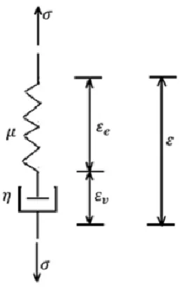
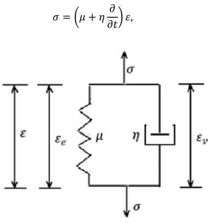
2.2.2.3 Kelvin-Voigt model
The Kelvin-Voigt model [9, 46] combines a spring and a dashpot in parallel, as shown in figure
2-6. For this model, the strain for the dashpot and the spring are equal, and the total stress for
the element is the sum of the stress on the spring and the dashpot, which gives the following
= + , (2.31)
Figure 2-6 The Kelvin-Voigt model.
Under constant stress, the model can predict the creep scenario. However, the limitation
of the model is that its capacity in the prediction of relaxation is less accurate. Once the material
parameters are determined through data fitting, these models could be used to describe the
linear viscoelastic behavior of materials.
2.2.2.4 Generalized models
Maxwell and Kelvin-Voigt models are good for qualitative and conceptual analysis, but as
indicated by Tobolsky and Andrew [45] that single Maxwell or Kelvin-Voigt element is not
enough to describe the behavior of polymers or elastomers. Due to the considerable number
and variety of molecular chains, the material behavior can be better represented if more than
one element in parallel is used. These models may have Maxwell elements in parallel with a
spring or Kelvin-Voigt elements in series with either a spring or a damper, and are named as
Wiechert’s model or Generalized models [51]. Figure 2-7 shows the generalized Maxwell
Figure 2-7 (a) Generalized Maxwell model; (b) Generalized Kelvin model.
As was discussed in the previous section, for the mechanical analogies being used to
better reflect the behavior of any viscoelastic material, the models are put under the same
forcing as in one of the tests explained above. Their response is derived and then the results are
plotted against the experimental data. Number of chains varies until the experiment data can
be captured. Several types of generalized models are used to describe different materials in the
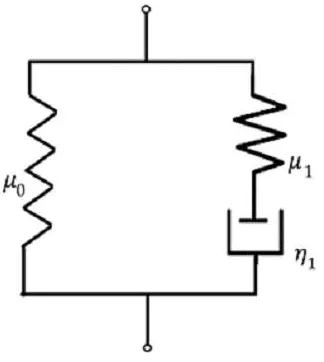
literature. One type of the generalized Maxwell models is called Zener model [52], which is
simply a single Maxwell element in parallel with a Hookean spring element as shown in figure
2-8 below.
Figure 2-8 The Zener model.
The relaxation or retardation time is defined as the ratio of the viscosity modulus for
the dashpot to the modulus of spring element of the Maxwell element [8, 9, 46], i.e.,
The expansion series used for the solution of generalized models is called Prony series
developed by Gaspard Riche de Prony [53].
2.2.3 Modeling of viscoelastic elastomers
One of the earliest works for modeling viscoelastic behavior of materials can be traced back to
Tobolsky and Andrews [45], where they worked on a molecular approach to describe the
mechanical behavior of such materials when classical theories of solid mechanics and fluid
mechanics were insufficient. Tobolsky and Andrew [45] focused majorly on rubbers, carrying
out several creep and relaxation tests to validate their models.
Later, Read [54] provided a method for stress analysis of compressible viscoelastic
materials. In this paper he proposed that the classical theory of elasticity could be used to
describe the time-dependent behavior of viscoelastic materials by utilizing mathematical tools
such as Fourier integrals. Such treatments could also be extended to anisotropic materials.
Lee [55] focused on the stress analysis of linear viscoelastic materials such as polymers
and plastics. Motivated by the mathematical problems and the increasing use of inelastic
materials. Lee published another work on the stress analysis of linear viscoelastic materials
later [56]. It was asserted in this paper that either differential or integral operators can be used
to define stress-strain relations for these materials, but it was more convenient to use integral
operators for creep and relaxation functions.
With the advent of nonlinear continuum mechanics in the early 1960’s, Coleman and
Noll [57] proposed fundamental assumptions for linear viscoelasticity. In their work, they
presented the theory of infinitesimal viscoelasticity based on the assumption that at
microscopic level the material could be represented by a combination of springs and dashpots
connected in complex networks. Further, they discussed the order of error in computing stress
when different theories were used for stress-strain constitutive relations. Pipkin [58] suggested
nonlinear integrals can be used to approximate the basic constitutive law for viscoelastic solids
subjected to small deformation under appropriate assumptions. Based on the work of other
researchers such as Green and Rivlin [59] and Noll [60], Pipkin reviewed the derivation of
these nonlinear integrals relating stress and strain, for isotropic and incompressible materials.
representation of nonlinear viscoelastic response to an arbitrary strain or stress history. They
tested their working on experimental data for tensile creep tests.
In 1968, Zienkiewicz and coworkers developed general numerical procedures for
solving broad range of viscoelastic problems [62]. Their research was mainly concerned with
creep analysis of concrete and rock. The finite element method for solving elastic problems has
been extended to account for the viscoelasticity. Later Taylor et al. also proposed numerical
procedures for solving linear viscoelasticity problems [63], in which they also took into account
the thermal effects.
Schapery[64] proposed a three-dimensional nonlinear constitutive model which was
aimed at the simulation of nonlinear responses of some metals and plastics. In this work various
methods of characterizing nonlinear viscoelastic solids were attempted.
Partom and Schanin [65] presented a nonlinear viscoelastic formulation based on the
generalized Maxwell model with linear springs and nonlinear dashpots. Their approach was
based on the evolution of the stresses and the internal state variables, which was used to predict
creep response for clamped beams under uniaxial loading. Such a procedure was claimed
simpler and more straightforward than the multiple and single integral representation adopted
in earlier works. Based on their work, Keren et al. [66] developed a finite difference code for
a two dimensional axisymmetric problem. Another approach to account for nonlinear
viscoelasticity was adopted by Rendell et al. [67] . This approach was based on the coupling
model of relaxation, which was found to better relate the viscoelastic behavior and features
observed during experiments with molecular theory. The simulations resulting from their
model revealed many key features observed through experimental strain histories.
In 1989 Gramoll et al. [68] developed a numerical procedure to solve nonlinear
viscoelastic problems of orthotropic materials such as fiber reinforced plastics (FRP) laminate
composites. However, their model was not sufficient to accurately predict the evolution of
strain and stresses over time. They further improved this numerical procedure by using Newton
Raphson method to solve the nonlinear problems, and further calibrated their numerical
simulation using experimental results. In the beginning of 1990s, Krishnaswamy et al.[69],
presented a finite algorithm to solve both linear and nonlinear problems for viscoelastic
response of materials. Their work was mainly focused on failure of material under cracks, and
materials. Kaliske and Rothert [70] also developed a formulation for three dimensional
viscoelasticity at small and finite strains based on the generalized Maxwell model for finite
element implementation. They presented simulations of time dependent deformations of rubber
structures.
Considering the lack of proper understanding and shortcomings in addressing
thermo-mechanical coupling, and large deformation in earlier work, Reese and Govindjee [71]
proposed a model for finite thermo-viscoelasticity. This model was claimed to be physically
reasonable and numerically tractable. Masuero and Creus [72] worked on nonlinearities caused in materials due to cracks and notches by developing nonlinear viscoelastic finite
element model to simulate the behavior of the material. This work was based on Schapery’s
[62]nonlinear viscoelastic formulation.
A comprehensive review on the nonlinear constitutive laws in viscoelasticity was
conducted by Drapaca et al. [73] and Wineman [74]. Drapaca et al. gave a review of classical
representation of continuum laws for viscoelastic materials, whereas Wineman reviewed all
aspects of modeling in viscoelastic materials from a phenomenological stand point. It was
concluded by Wineman that there were no generally accepted well-defined forms of
CHAPTER 3
3
Finite element modeling for linear viscoelastic
response
In this chapter, formulation for the linear response of viscoelastomers is developed based on a
generalized Maxwell rheological model. Moreover, the developed formulation is implemented
in ABAQUS CAE as a user material subroutine (UMAT). A comparison between the
simulation result from the UMAT and the experimental data of a uniaxial tensile test is also
given in this chapter. Furthermore, the robustness of the developed UMAT is tested by
simulating viscoelastomers subjected to complex loads.
3.1 Basic theory
The basic theory of linear viscoelasticity is introduced below, which will lead to a better
understanding of the formulation for finite element implementation.
3.1.1 Stress and strain
The response of viscoelastomers is strongly affected by its intrinsic viscous and elastic
properties. The response of a material is the way the material deforms under the application of
a load. Consider a reference configuration (undeformed and stress-free) of an elastomer, the
material point in this configuration is identified by the position vector . After deformation the
current position of this material point is given by = ( , ), where describes the motion of
material point from the reference to the current configuration. The deformation gradient [75]
is defined as follows:
= , =
⎣ ⎢ ⎢ ⎢ ⎢ ⎢ ⎡
⎦ ⎥ ⎥ ⎥ ⎥ ⎥ ⎤
= . (3.1)
= ( + )= + . (3.2)
Under deformation, the stress of the material can be expressed as Cauchy stress (true stress) or first Piola-Kirchoff stress P (nominal stress). With the deformation gradient tensor
F, these two stresses are interconvertible, i.e.,
= . (3.3)
Here is the determinant of the deformation tensor and is the inverse of the deformation
tensor .
3.1.2 Boltzmann superposition principle
According to the superposition principle, for all linear systems, the net response caused by
multiple stimuli can be regarded as the sum of the responses caused by each individual
stimulus. In other words, if an input to function produces a response X and an input
produces a response Y, then input ( + ) produces response (X + Y) [47], i.e.,
X + Y = ( + ) = ( ) + ( ). (3.4)
3.2 Numerical formulation for linear response of
elastomers
This section is focused on developing a generic three-dimension formulation for linear
response of a viscoelastomer, which is structured based on the work of Kaliske and Rothert
[70]. The formulation is derived based on a generalized Maxwell rheological model. First, a
one-dimension modeling framework for small strain of viscoelastic solids is revisited. Then a
three-dimensional formulation for finite element simulation of viscoelastomers is proposed.
For a single Maxwell element (see figure 2-5), the stress-strain relation (as first given
in equation (2.30)) can also be expressed as
̇ +1 = ̇. (3.5)
= exp − . (3.6)
The value of the constant is determined by the initial conditions. When a relaxation test is
considered, i.e., (0) = ( ) = constant, figure 3-1 shows the stress response of the material
under such a relaxation test [70].
Figure 3-1 Relaxation test of a Maxwell element [70]
From figure 3-1, the initial stress on the material is governed by the elastic response,
i.e., at time = 0 the stress on the material is (0) = (0).With this initial condition,
constant C in the homogenous solution can be solved. Since the strain in the experiment is
constant, i.e., the strain rate is zero, it leads to the particular solution of equation (3.5) as =
0. Thus, the solution of equation (3.5) is determined as
( ) = exp − (0). (3.7)
Here the relaxation function is defined as
Г( ) = exp − , (3.8)
which indicates the viscoelastic characteristics of the material. The above derivation can be
extended to a generalized Maxwell model, see figure 2-7 (a). Let the modulus of the spring
element parallel to the Maxwell elements be and the moduli for the spring components of
the Maxwell elements be , , … , where is the total number of Maxwell elements as
given as , , … . The overall stress acting on the generalized model is equal to the
sum of the stresses acting on the Hookean spring and the parallel Maxwell elements. Adopting
the generalized Maxwell model, the stress of the material is expressed as
( ) = (0) + exp − (0) = Г( ) (0).
(3.9)
Here is the relaxation time for each Maxwell element, which equals to the ratio of viscosity
constant for each damper to the modulus of the spring in the Maxwell element. The relaxation
function becomes
Г( ) = + exp − .
(3.10)
A normalized form of the relaxation function is given below as
( ) =Г( )= 1 + exp − .
(3.11)
Here is the ratio of to . For incremental strain ∆ of the material, the Cauchy stress is
expressed as
( ) = Г( − ) . (3.12)
Here the initial response commences at any time . Although only the relaxation of the material
is considered, a very similar formulation can also be obtained for the creep test. For equation
(3.12), the relaxation function Г( − ) is given as
Г( − ) = + exp (− − )
(3.13)
Expanding equation (3.12), the stress is written as
( ) = ( ) + exp − − ( ) .
Figure 3-2 Generalized Maxwell rheological model with N Maxwell chains.
Since is a constant and the sum of all the responses for strain ( ) over the time is ( ),
equation (3.14) is thus rewritten as
( ) = ( ) + − − ( ) , (3.15)
resulting in
( ) = ( ) + ℎ ( ) (3.16)
Here ( ) is the stress for the elastic element (the Hookean spring), and ℎ ( ) defines the
internal stresses in the Maxwell elements, i.e.,
ℎ ( ) = exp − − ( ) (3.17)
From equations (3.15) and (3.16), and ( ) = ( )/ , equation (3.17) can be expressed in
the other format as,
ℎ ( ) = exp − − ( ) . (3.18)
In a relaxation test, the internal stress variable ℎ ( ) approaches to zero if the time
approaches infinity [70]. This means that under a constant deformation, the stress on the
material will eventually relax to the value of the elastic portion (
lim
In the formulation below, a finite difference method is applied to equation (3.18) to
determine ℎ ( ) [70]. Consider a time interval [ , ] and a time step ∆ = − , the
multiplicative split of the exponential term leads to
exp − = exp − + ∆ = exp − exp −∆ . (3.19)
For the defined time interval, the deformation is kept constant for each time increment from
to . Thus, stress is only a function of time. Integrating equation (3.18) up to time
results in,
ℎ ( ) = exp −( − ) ( ) . (3.20)
The deformation history can be separated into two steps, i.e., from 0 ≤ ≤ and from ≤
≤ , which further leads to the following formulation,
ℎ ( ) = exp −( − ) ( )
+ exp −( − ) ( ) .
(3.21)
Since ∆ = − , equation (3.21) can be rewritten as
ℎ ( ) = exp −∆ exp − − ( )
+ exp − − ( ) .
(3.22)
Comparing equation (3.22) and equation (3.18), we can find that
ℎ ( ) = exp −( − ) ( ) . (3.23)
Therefore equation (3.22) is written as
ℎ ( ) = exp −∆ ℎ ( ) + exp − − ( ) . (3.24)
The integral in the above equation can be simplified using a similar finite difference approach
on ( ), i.e.,
( ) = lim
∆ →
∆ ( )
∆ = lim∆ →
−
∆ . (3.25)
Introducing the time discretized approximation of the second order into the formula, a
ℎ = exp −∆ ℎ +
1 − exp −∆
∆ [ − ].
(3.26)
This indicates that all the values for ℎ ( ) are dependent on the preceding values of ℎ . If those
values are known, subsequent values for any given time step can be determined using the
iterative formulation shown in equation (3.26). Utilizing the iterative formulation equation
(3.16) becomes
= + ℎ , (3.27)
which defines a one-dimensional numerical formulation for a linear response of
viscoelastomers. One can observe that the relaxation function has been replaced by an
exponential series which is dependent on individual moduli of spring and damper in the model.
To introduce the three-dimension formulation, tensor notation is adopted in equation
(3.27), i.e.,
= + ℎ . (3.28)
Here the elastic stress is defined as
= . (3.29)
The superscript in emphasizes that this tensor describes an elastic relation between the
stress and the strain. The fourth order tensor is the stiffness matrix which is defined by
generalized Hooke’s law for elastic materials [76]. The formulation derived above is based on
the following assumptions: 1) the material under consideration is linear in nature, i.e., its
stiffness is constant; 2) the deformation the material undergoes is also linear, i.e., Boltzmann
superposition, Hookean and Newtonian principles for linearity apply; 3) the material is
homogenous and isotropic. Consider that the Voigt notation [77] is convenient to use, it is
introduced here and leads to
= , (3.30)
= ⎣ ⎢ ⎢ ⎢ ⎢ ⎡ ⎦ ⎥ ⎥ ⎥ ⎥ ⎤ , (3.31)
with = , = , = , = = , = = , = =
. Similarly, the strain tensor with Voigt notation is given as
= ⎣ ⎢ ⎢ ⎢ ⎢ ⎡ ⎦ ⎥ ⎥ ⎥ ⎥ ⎤ . (3.32)
The stiffness matrix defines the relation between elastic stress and strain, which takes the
form for the isotropic material as
= ⎣ ⎢ ⎢ ⎢ ⎢
⎡ 00 00 00
0 0 0
0 0 0 0 0
0 0 0 0 0
0 0 0 0 0 ⎦
⎥ ⎥ ⎥ ⎥ ⎤ = ⎣ ⎢ ⎢ ⎢ ⎢
⎡ + 2 + 2 00 00 00
+ 2 0 0 0
0 0 0 0 0
0 0 0 0 0
0 0 0 0 0 ⎦
⎥ ⎥ ⎥ ⎥ ⎤ , (3.33)
where and are Lame’s constants [78]. Also, 3 = 3 + 2 with being the bulk modulus
of the material. Thus, the internal stress variables in equation (3.26) can be rewritten as
ℎ = exp −∆ ℎ +
1 − exp −∆
∆ [ − ].
(3.34)
Expanding equation (3.28), the incremental formulation for the Cauchy stress is given as
=
+ exp −∆ ℎ +
1 − exp −∆
∆ [ − ].
Equation (3.35) provides an iterative formulation for the stress of a viscoelastic
material. Using this formulation, a user material subroutine (UMAT) will be developed to solve
complex problems using FEM software like ABAQUS CAE.
3.3 Development of UMAT for linear viscoelastic response
A UMAT is a user material subroutine that defines a constitutive relation of the material.
Details and format of UMATs can be found in the ABAQUS/ STANDARD manuals and
subroutine guides [78, 79].
3.3.1 Formulation of UMAT for linear viscoelastic analysis
The development of the UMAT is based on constitutive equation (3.35). Three essentials are
required to complete a UMAT, including defining the material parameters, the constitutive
equation and the material Jacobian matrix.
Stress-strain constitutive equation
In this case study, we only consider three Maxwell elements in parallel with the Hookean
spring. Therefore, the constitutive equation (3.35) is expressed as
= + exp −∆ ℎ + exp −∆ ℎ + exp −∆ ℎ
+ 1 +
1 − exp −∆
∆ +
1 − exp −∆
∆
+
1 − exp −∆
∆ [ ∆ ],
(3.36)
where ∆ = − .
State variables
In the development of the generalized formulation we used a state variable approach [46],
where we replaced the relaxation function with an approximated exponential series. The
internal stresses in the Maxwell elements given by the function ℎ are defined as state variables
in the UMAT. These stresses will be updated in each iteration using the relation defined by
Stiffness matrix
The Lame’s constants described in previous section satisfy 3 = 3 + 2 . Here = . So,
= − . Hence, as per equation (3.33) the stiffness matrix for the elastic component of
the model is given as
= ( , ) = ⎣ ⎢ ⎢ ⎢ ⎢ ⎢ ⎢ ⎢ ⎡ +4
3 −
2
3 −
2
3 0 0 0
−2
3 +
4
3 −
2
3 0 0 0
−2
3 −
2
3 +
4
3 0 0 0
0 0 0 0 0
0 0 0 0 0
0 0 0 0 0 ⎦
⎥ ⎥ ⎥ ⎥ ⎥ ⎥ ⎥ ⎤ . (3.37)
Jacobian matrix
The material Jacobian which is also known as the tangent modulus is the slope for the
stress-strain curve obtained from the constitutive equation. It is the requirement for ABAQUS/
STANDARD UMAT only [78]. For a small deformation problem, or a large deformation
problem with no or very little volume change (incompressible material), the Jacobian is
calculated by ∆
∆ [78, 79]. Here, ∆ is a small increment in Cauchy stress and ∆ is the
increment in strain. The matrix formed may be non-symmetric and depends on the constitutive
equation for stress and strain. In this case, equation (3.36) is used to calculate the Jacobian
matrix, i.e.,
ℂ = ∆
∆ = 1 +
1 − exp −∆
∆ , (3.38)
where is the stiffness matrix defined in equation (3.37).
UMAT code
The UMAT code is given below, with detailed interpretation given in Appendix.
C************************************************************************************* ********
C* This UMAT is based on generalized Maxwell model with three Maxwell element chains.
C************************************************************************************* ***
SUBROUTINE UMAT(STRESS,STATEV,DDSDDE,SSE,SPD,SCD,
1 RPL,DDSDDT,DRPLDE,DRPLDT,
2 STRAN,DSTRAN,TIME,DTIME,TEMP,DTEMP,PREDEF,DPRED,CMNAME, 3 NDI,NSHR,NTENS,NSTATEV,PROPS,NPROPS,COORDS,DROT,PNEWDT, 4 CELENT,DFGRD0,DFGRD1,NOEL,NPT,LAYER,KSPT,KSTEP,KINC) C
INCLUDE 'ABA_PARAM.INC' C
CHARACTER*8 CMNAME
DIMENSION STRESS(NTENS),STATEV(NSTATEV),
1 DDSDDE(NTENS,NTENS),DDSDDT(NTENS),DRPLDE(NTENS), 2 STRAN(NTENS),DSTRAN(NTENS),TIME(2),PREDEF(1),DPRED(1), 3 PROPS(NPROPS),COORDS(3),DROT(3,3),DFGRD0(3,3),DFGRD1(3,3) DIMENSION D(3,3), SM1OLD(6), SM2OLD(6), SM3OLD(6),
1 SM1(6), SM2(6), SM3(6), SM1DOT(6), SM2DOT(6), SM3DOT(6), G(6,6) REAL*8 M1,M2,M3
C
C PROPS(1) THROUGH PROPS(3) ARE THE SHEAR MODULI IN PASCALS C MU0=PROPS(1)=14.59E3
C MU1=PROPS(2)=11.87E3 C MU2=PROPS(3)=41.35E3 C MU3=PROPS(4)=19.75E3
C PROPS(5) THROUGH PROPS(7) ARE THE RELAXATION TIMES IN SECONDS C TAU1=PROPS(5)=960.4
C TAU2=PROPS(6)=1.044 C TAU3=PROPS(7)=19.3
C PROPS(8) IS THE BULK MODULUS OF THE MATERIAL=10^3*PROPS(1) C PROPS(8)=14590E3
C C
C DEFINING STATE VARIABLES FOR INTERNAL STRESSES FOR MAXWELL ELEMENTS C DO I=1,6 SM1OLD(I)=STATEV(I) ENDDO DO I=1,6 SM2OLD(I)=STATEV(I+6) ENDDO DO I=1,6 SM3OLD(I)=STATEV(I+12) ENDDO C
C DEFINING THE VALUES FOR M1, M2 AND M3 C
C
M1=(PROPS(5)*PROPS(2)-
1 PROPS(5)*PROPS(2)*EXP(-DTIME/PROPS(5)))/(PROPS(1)*DTIME) M2=(PROPS(6)*PROPS(3)-
1 PROPS(6)*PROPS(3)*EXP(-DTIME/PROPS(6)))/(PROPS(1)*DTIME) M3=(PROPS(7)*PROPS(4)-
1 PROPS(7)*PROPS(4)*EXP(-DTIME/PROPS(7)))/(PROPS(1)*DTIME) C
C DEFINING THE TERMS TO BE USED IN STIFFNESS MATRIX C
![Figure 2-2 Relaxation test for a viscoelastic material [10].](https://thumb-us.123doks.com/thumbv2/123dok_us/1923178.1252461/23.612.116.484.136.444/figure-relaxation-test-for-a-viscoelastic-material.webp)
![Figure 2-3 Creep test for a viscoelastic material [10].](https://thumb-us.123doks.com/thumbv2/123dok_us/1923178.1252461/24.612.175.425.121.355/figure-creep-test-a-viscoelastic-material.webp)
![Figure 3-1 Relaxation test of a Maxwell element [70]](https://thumb-us.123doks.com/thumbv2/123dok_us/1923178.1252461/34.612.206.413.176.386/figure-relaxation-test-maxwell-element.webp)