Cabray L. Haines is a former senior associate economist and Richard J. Rosen is a senior economist and economic advisor in the Economic Research Department of the Federal Reserve Bank of Chicago.
Introduction and summary
Home prices have been in the news a lot lately. In particular, some observers fear that the swift increase in prices during the early part of the new century may have constituted a housing price bubble.1 This con-cern has been prompted primarily by the rapidity of the rise, both compared with previous years and rela-tive to growth in rents.2 The home price increases, how-ever, occurred during a period of rising incomes and falling mortgage rates. The changes in both income and mortgage rates made housing more affordable and should therefore have led to higher home prices, all else being equal. In this article, we document changes in prices for the country as a whole and for many major markets. We examine whether changes in the economy, including income and mortgage rates, are enough to ex-plain home price changes, both nationally and locally.
To determine whether there has been a bubble— and whether the bubble is bursting—we need to know what home prices “should” be. We use data from 1980 through (midyear) 2006 to create a simple reduced-form model of single-family home prices. Our focus is on the relationship between home prices and mort-gages rates. We use a metric that measures the fraction of income necessary to cover the mortgage payments
on a home. We find that this metric helps explain
home prices and that, as expected, falling mortgage rates are associated with higher prices.
Our sample period includes times when home prices were growing rapidly and times when they were not. One focus of this article is to determine whether the past few years are truly different from prior years, that is, whether there is a housing bubble, either in the nation as a whole or in selected markets. As noted, in recent years, home prices have increased more than rents. We show that they have also creased relative to changes in mortgage rates and in-come. When we estimate our regression model, we
find that, on average, home prices are above their pre -dicted levels in the post-1999 part of our sample. How-ever, this result does not hold true uniformly across the country. Markets on the coasts, especially those in California, Florida, and the Northeast, have prices
significantly above predicted levels. Some other markets
have prices below predicted levels. Thus, to the extent that prices have been overheating, the phenomenon is limited to some markets, many of which have
tradition-ally exhibited volatile prices. Still, if factors such as
the recent increases in mortgage rates cause prices to move toward their predicted levels, there could be
significant corrections on the horizon in some markets. When we focus on the Seventh Federal Reserve
District,3 we find little evidence of a housing price bubble. Home prices in the larger markets in the
Seventh District show some volatility, but are gener -ally in line with other markets in the interior of the country. In the smaller markets, home prices have not deviated much from their predicted values. Background
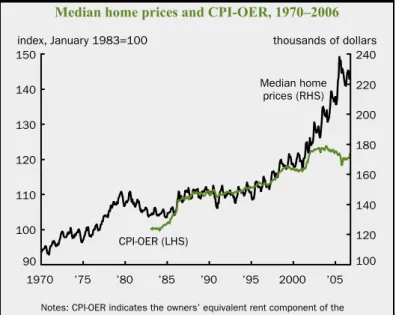
Figure 1 charts the median sale price of an
exist-ing U.S. sexist-ingle-family home over the last 36 years
(all dollar values are in constant 2006 dollars).4 Over the period, prices were generally increasing, except for several years in the early 1980s. The median home price was $118,500 in 1972. It increased to $148,700
in late 1980 before high mortgage rates and inflation
pushed prices down. Prices fell through 1984, reaching a minimum of $131,400 near the end of that year. There then was a period of moderate price increases
Bubble, bubble, toil, and trouble
A. FIguRE 1
Median home prices and CPI-OER, 1970–2006
1970 ’75 ’80 ’85 ’90 ’95 2000 ’05 90 100 110 120 130 140 150 100 120 140 160 180 200 220 240
index, January 1983=100 thousands of dollars
Notes: CPI-OER indicates the owners’ equivalent rent component of the Consumer Price Index. LHS means left-hand scale. RHS means right- hand scale. All dollar values are in constant 2006 dollars. Sources: National Association of Realtors and U.S. Bureau of Labor Statistics from Haver Analytics.
Median home prices (RHS)
CPI-OER (LHS)
from 1984 through 1994, with prices increasing at a 1.2 percent annual rate. After that, prices increased at an accelerating pace through 2000, rising at 2.1 per-cent per year; at the end of 2000, the median home price was $169,400. This increase was similar to that of the 1970s. But starting around the turn of the cen-tury, the rise in home prices really began to accelerate. Prices went up at an annual rate of 7.9 percent from the end of 2000 to their peak of $238,600 in June
2005. Some believe that the rapid increase in housing
prices is a sign of a bubble.5 From June 2005 through August 2006, prices fell 6.6 percent, which some saw as the beginning of the end of the alleged bubble.6
As a first pass at determining whether prices are
too high, we can break the value of owning a home into two parts. An owner-occupied house combines a
flow of services with an investment good. The home -owner gets to live in the house in lieu of renting a simi-lar unit and also gets a potential return on the equity in the house. In a stable market, the return on home equity should parallel that of other investments with
a similar risk profile. That is, one should compare the
sum of the return plus the rental value of living in the home to the return on other similarly risky investments. One way to decompose the change in home prices into the rental equivalent portion and the return on equity portion is to compare home prices with rental prices. We use the owners’ equivalent rent component
of the Consumer Price Index (henceforth, CPI-OER)
as a proxy for the stream of earnings from renting a house.7 The ratio of the median sale price of an existing
single-family home to CPI-OER gives a picture
of home buyers’ expectations of price ap-preciation on their purchases. This is, in essence, a price-to-earnings ratio (Leamer, 2002). Home prices rising much faster than the stream of rental income could be a sign that a bubble is forming, or at least that prices are rising faster than funda-mentals.
Figure 1 compares the evolution of
the CPI-OER since its inception in 1983 with that of home prices. As the figure
shows, home prices and the rental index moved together until the late 1990s. At that point, the rate of increase in prices began to exceed the change in the rent in-dex by a substantial margin. Even so, this shift may be misleading, since housing markets are by their nature local, and ex-amining national trends can miss impor-tant differences across markets. Indeed,
prices vary significantly between localities. To illus
-trate, figure 2 graphs the median sale price of an ex
-isting single-family home in San Francisco, Chicago,
and Kansas City, three major metropolitan markets (where markets are metropolitan statistical areas, or
MSAs). Prices went up in all three markets, but not at
the same rate. Home prices in Chicago rose at a 0.8 percent annual rate through 2000, before shooting up
7.3 percent per year after that. Prices in San Francisco
went up more consistently and at a faster pace than in the other two markets prior to 2000, rising at a 3.7 percent annual pace from 1980 through 2000 and then increasing at a 6.3 percent pace from 2000 on. Kansas City, on the other hand, has seen prices rise more slow-ly in the last few years—at onslow-ly a 0.9 percent annual
rate. Some observers have taken the rapid increases in price in markets such as Chicago and San Francisco
as an indication of overheated prices.8 However, these results do not necessarily mean that there is a housing
bubble in San Francisco or Chicago and that housing
prices are too low in Kansas City. They do, however, suggest that we need to examine prices on a local level, as most studies of housing do.
Literature review
A number of researchers have asked whether in-creases in home prices or the price-to-rent ratio mean that prices are too high.9 One of the first studies to examine a large sample of home prices found that
A. FIguRE 2
Median home prices for selected metropolitan statistical areas, 1980–2006 0 200 400 600 800 1980 ’82 ’84 ’86 ’88 ’90 ’92 ’94 ’96 ’98 2000 ’02 ’04 ’06 thousands of dollars San Francisco, CA Chicago, IL Kansas City, MO
Note: All dollar values are in constant 2006 dollars. Source: National Association of Realtors from Haver Analytics.
year-to-year price changes in the 1970s and 1980s were correlated, and that prices at any given time did
not fully reflect all available information, such as in
-terest rates (Case and Shiller, 1989). That left open
the possibility that home prices in the 1980s were too high. Could the momentum resulting from the price correlation lead to a bubble?
More recent research has addressed the question of whether home prices are too high and whether there is a bubble in the context of the recent run-up in price. These papers typically start with a model of what home prices should be or how they should change. In doing so, the studies fall into two groups. One group decon-structs the price of a home into its constituent parts (for
example, Himmelberg, Mayer, and Sinai, 2005). The
cost of owning a home is a function of the foregone interest from the funds used to buy the home; the net tax impact of owning, depreciation, and maintenance; a risk premium for owning rather than renting; and any transaction costs. Deducting any expected capital gains gives the “imputed rent,” which is an estimate of the
benefit of living in the house plus any mispricing. If
this imputed rent is high relative to actual rents, then
a home can be said to be overvalued. Studies that de
-construct home prices like this typically find, at most,
limited overpricing in the last decade (for example,
Himmelberg, Mayer, and Sinai, 2005; McCarthy and Peach, 2004; and Smith and Smith, 2006). One issue
with models like this is that they are sensitive to assump-tions, especially regarding the expected capital gains.
Other studies estimate reduced-form models, looking for correlations between home prices and factors that are likely to
influence the supply or demand for hous -ing. For example, when incomes rise, households may be able to afford to spend more on homes. Thus, a number of stud-ies have tested whether home prices (or their changes) are correlated with income (or its changes). In general, prices seem to rise with income (see, for example, Case
and Shiller, 2003; and Lamont and Stein,
1999).10 Other factors, such as interest (mortgage) rates and population, also can affect home prices. The limitation of pa-pers of this type is that they are reduced forms rather than structural models. Thus,
if the models are not carefully specified,
the correlations they estimate can be
spu-rious. Still, these models find little evi -dence of across-the-board overpricing.
Since home prices are at least partial -ly driven by factors in a local market, virtual-ly every study estimates prices at the state or metropolitan
market level. Some studies find evidence that homes
in selected local markets are overpriced (for example,
Case and Shiller, 2003; and Himmelberg, Mayer, and Sinai, 2005), but others claim that there is not signifi -cant overpricing (for example, McCarthy and Peach, 2004). In the papers that found some overpricing, the areas where prices were estimated to be “too high” were often locations where the ability to build new houses was limited relative to demand. There is
evi-dence that zoning restrictions are associated with high
prices and that prices may behave differently in “superstar” cities than in other areas (Glaeser, Gyourko,
and Saks, 2005; and Gyourko, Mayer, and Sinai, 2006).
This brings up a related point that where homeowners are subject to more risk, prices may be more sensitive
to shocks (Lamont and Stein, 1999; and Sinai and Souleles, 2003). Homeowners may be subject to
more risk where homes are expensive (leading to homeowners having higher leverage) or where de-mand is inelastic, such as in superstar cities (McCarthy and Peach, 2004). Thus, what appears to be a bubble
in some markets might just be a reflection of normal -ly high volatility in those markets.
The general consensus of the academic literature is that home prices are largely in line with fundamen-tals. Overpriced markets, if any, are limited in num-ber and in the scope of overpricing. This is in contrast to some nonacademic studies. For example, one re-cent analysis found that markets accounting for
A. FIguRE 3
Mortgage-servicing index and average mortgage rates, 1972–2006 0 10 20 30 40 50 0 5 10 15 20 1972 ’76 ’80 ’84 ’88 ’92 ’96 2000 ’04 percent percent Average mortgage rate (RHS) Mortgage-servicing index (LHS)
Notes: LHS means left-hand scale. RHS means right-hand scale. The construction of the mortgage-servicing index is described in the text. Sources: Authors’ calculations based on data from the National Association of Realtors, Freddie Mac, and U.S. Bureau of Labor Statistics from Haver Analytics.
40 percent of all single-family home value are over-priced by at least 34 percent (Global Insight and National City Corporation, 2006). Of course, this disparity may exist because of the lags that are com-mon to getting academic studies published. The non-academic studies include data through 2005 and into 2006, while few of the academic studies include the more recent data. One contribution of our study is that we include data through midyear 2006. This helps us to determine whether the differences be-tween the academic and nonacademic research are a function of the approach or of the period studied. Home prices and mortgage rates
To determine whether home prices are too high, we need to have an estimate of what they should be. In this article, we use a reduced-form model to estimate home prices. As a start, in this section, we explore a simple relationship between prices and mortgage rates.
During the recent increase in home prices, long-term interest rates, including mortgage rates, were de-clining to very low levels.11 If potential homeowners determine the price they are willing to pay based on
the size of the mortgage payment it generates, then
lower interest rates can lead to higher home prices.
To estimate this effect, we define the mortgage-ser
-vicing index (MSI) to be the ratio of the mortgage
payment on the median-priced existing single-family home to the median household income, where we as-sume that home buyers use a down
pay-ment equal to 20 percent of the purchase
price and finance the rest of the transac
-tion with a 30-year fixed-rate mortgage (Rosen, 2005).12 The index reflects the proportion of income necessary to make mortgage payments, and lower values of the index signal that housing is more af-fordable.13 Figure 3 graphs the MSI since 1972, along with the average interest rate
on a 30-year fixed-rate mortgage for ref -erence. Viewed through this lens, housing has become less affordable recently (that is, the index is higher) after a period of relatively affordable prices over the last 15 years. It took about 26.8 percent of the median household’s income to pay the mortgage on a house with the median sale price in 2005. This was the highest value of the index since 1991. As mortgage rates have continued to trend slightly up in
2006, the MSI has continued to rise. This
has occurred, even though housing prices have begun to decline. As of June 2006,
the MSI was approximately 28.3 percent. The last time the MSI was significantly higher was
a result of the run-up in mortgage rates in the late 1970s, after which the index remained elevated until
mortgage rates had declined for about five years.
The past few years are somewhat reminiscent of the late 1970s in another way. Mortgage rates started rising in 1978, and real housing prices continued to
rise for two more years. Similarly, mortgage rates have
been inching up in the last two years, but real housing prices have continued to climb rapidly. This has led
to a big increase in the MSI, indicating decreased hous -ing affordability. One issue is whether real hous-ing prices will start to decline as they did in the early 1980s. It is important to note one big difference be-tween the last few years and the late 1970s–early 1980s
period: Inflation was high then and is relatively low
now. In the earlier period, nominal housing prices rose but real prices fell. Now, there is much less scope for a decline in real prices if nominal prices do not fall.
Since there is some belief that housing prices are slow
to react to downward pressure, this may make a signif-icant downward shift in real housing prices less likely.
The 1994 increases in interest rates also offer ev-idence on—and a possible alternative for—what will happen to housing prices. Mortgage rates rose from 7.3 percent in 1993 to 8.4 percent in 1994, leading to
an increase in the MSI from 23.1 percent in 1993 to
signaled that housing was less affordable in 1994 than in 1993, this quickly reversed, with affordability in-creasing in 1995 as the index declined to 24.1 percent. The index remained roughly at that level through 2004, even as housing prices rose. Two differences between the mid-1990s and the late 1970s–early 1980s periods are that the increases in mortgage rates were
tempo-rary and that inflation did not increase. This implies
that if the increase in mortgage rates in recent months is not sustained, housing affordability may revert to its previous level.
Model of predicted housing prices
Figure 3 suggests that housing prices might respond to changes in mortgage rates and income levels. This section introduces other factors that can help explain housing price changes. Our objective is to set out a model of predicted housing prices and use that model to determine whether housing prices were above their
predicted level in the early part of this decade. Since
housing markets are by their nature local, and examin-ing national trends can miss important differences across markets, we examine local markets. As
men-tioned previously, we define local markets as metro -politan statistical areas, and we include 43 of the
largest MSAs in our sample.
A number of the factors that we use to explain housing prices are related to each other, so we use re-gression analysis to predict housing prices. We em-ploy a reduced-form model similar to previous work
(especially Case and Shiller, 2003), but with a special
focus on mortgage affordability. The baseline empiri-cal model is:
1) HOME PRICE = f(AFFORDABILITY INDEX, other controls),
where we pool annual data for our 43 local markets. The home price series used for our results is based on the
U.S. Office of Federal Housing Enterprise Oversight (OFHEO) index (adjusted for inflation). The OFHEO
index is a repeat sales measure of single-family home prices, so it is less vulnerable to changes in the stock of homes than is the median sale price of an existing home. It also is among the longest time series of home
prices available for a large number of MSAs. To con -vert the index to a dollar-value equivalent, we set the 1980 value of our home price index to equal the me-dian sale price of an existing single-family home at that time (the results are similar using other years, or the sample mean, as the base). We then compute sub-sequent years’ index values by using the percentage change in the OFHEO index.
We now describe the other variables in our anal-ysis, which, with the exception of the affordability in-dex, are drawn from previous studies of housing prices. Table 1 presents summary statistics for our sample.
The affordability index is designed to be a cousin
of the MSI. Since the MSI is calculated using home
prices, we do not want to use it as a right-hand side variable in our regressions. However, we want to in-clude the effect of interest rates on the affordability
of a home. We define theAFFORDABILITY INDEX as median household income divided by the yearly
payment on a fixed-rate 30-year $100,000 mortgage
with a 20 percent down payment. This is inversely
re-lated to the MSI. When mortgage rates fall, the af -fordability index increases and it becomes easier for a potential owner to afford a house at a given price.
In contrast, a lower value of the MSI indicates greater
affordability.
TaBLE 1
Summary statistics for the sample, 1980–2006
Standard
Variable Mean Median deviation
HOME PRICE (index) 161.65 137.46 79.56
AFFORDABILITY INDEX 6.71 6.62 2.13
INCOME ($ thousands) 50.19 49.22 7.02
UNEMPLOYMENT (percent) 5.55 5.24 1.89
POPULATION DENSITY (per square mile) 640.80 446.55 541.11
CONSTRUCTION COST (index) 4,210.27 4,128.19 185.34
MEDIAN AGE 33.62 33.60 2.78
Notes: The home price in year t is derived from the median price of an existing single-family home in 1980 augmented by the change in the U.S. Office of Federal Housing Enterprise Oversight’s repeat-sale home index between 1980 and year t. The affordability index is the median household income divided by the payment on a $100,000, 20 percent down, 30-year fixed-rate mortgage. Income is the median annual household income. Construction cost is the Engineering News-Record’s national Building Cost Index. All variables except construction cost (and the mortgage rate) are for the local market. All dollar values are in constant 2006 dollars.
Sources: Authors’ calculations based on data from the National Association of Realtors, U.S. Office of Federal Housing Enterprise Oversight, Freddie Mac, U.S. Bureau of Labor Statistics, U.S. Census Bureau, Engineering News-Record, and Haver Analytics.
In addition to the affordability index, we include two other measures of households’ ability to pay for a home. As mentioned earlier, previous studies have noted that prices are correlated with income (for example,
Case and Shiller, 2003). Income enters the affordabil -ity index, since higher incomes mean that, all else be-ing equal, a household can afford a more expensive home. However, it is possible that income exerts an independent effect on prices. A wealthier household may have more disposable income and may therefore choose to consume more housing. For this reason, we include INCOME, the median household income in a market, as a control. Also, UNEMPLOYMENT, the
unemployment rate in an MSA (as reported by the U.S. Bureau of Labor Statistics), is included to pick
up local economic conditions. When there is a lot of employment, demand for housing is likely to be high.
The population characteristics in a market may affect both the supply and demand for housing. A grow-ing population may indicate an increasgrow-ing demand for housing. Also, a densely populated market is
consis-tent with difficulties in building new housing because
land is scarce. Hence, greater population density might indicate housing supply limitations. To capture this, we include POPULATION DENSITY, the population per square mile in a market, as a control variable. In addition, the age distribution of a population may af-fect home prices, as different age groups have differ-ent housing needs and may be more or less willing to pay for housing. We include the variable MEDIAN AGE, the median age of the population (available only at the state level), to probe such effects.
Another factor that might influence home prices
is the cost of construction. We use CONSTRUCTION COST, the national Building Cost Index published monthly by the Engineering News-Record. Previous
housing studies have also used this index (Somerville,
1999). Unfortunately, it is not available for all markets in our sample, so we use the national index.
Finally, there are some factors that influence home
prices that we cannot directly control for because of data limitations. For example, there is evidence that land supply issues affect home prices. In areas with
tight land supply, imposing strict zoning constraints
increases prices (for example, Glaeser, Gyourko, and
Saks, 2005). In general, the ratio of land values to home
values affects the variability of home prices (Bostic,
Longhofer, and Redfearn, 2006). Additionally, there
is evidence that income dispersion can affect home prices (Van Nieuwerburgh and Weill, 2006). We par-tially address these concerns by including market
dummy variables (that is, MSA fixed effects) in many
of our regressions. This controls for the attractiveness
of superstar cities, as well as any land supply, zoning
constraints, or income dispersion differences that are not picked up by other variables. The implicit assump-tion is that these characteristics do not change over the sample period, something we return to later in this article.
Table 2 presents the results of regressions of home prices on the affordability index and controls. The regression in column 1 includes only the index on the right-hand side. The results indicate that when lower mortgage rates or higher income make housing more affordable, prices increase. The regression in column 2 adds in the other control variables. The
co-efficient on AFFORDABILITY INDEX is smaller in
magnitude than in the first regression, but still posi
-tive and significant. To evaluate the economic impact
of the index on home prices, we examine the effect on predicted prices when mortgage rates fall from 10 percent to 9 percent, given a household income of $50,000. This change increases AFFORDABILITY INDEX from 5.93 to 6.47, resulting in a predicted in-crease in HOME PRICE of 10.596 × (6.47 – 5.93) = 5.72. At the sample mean for HOME PRICE of 161.65, this translates to an increase in (real) home prices of 3.5 percent.
The other control variables in the regression gen-erally have the expected signs. Increasing household income raises home prices above and beyond income’s indirect effect on affordability. Higher construction costs are partially passed through to home prices. Higher population density is also associated with higher home prices. Finally, home prices rise as the median age of a market falls.
The first two regressions assume that any pricing
differences one market has compared with another are constant. However, it is possible that the reaction of the level of home prices to changes in affordability and income is related to how expensive housing is in that market. To put it another way, the level of home prices might be more sensitive to changes in affordabili-ty and income in expensive superstar markets than in less expensive markets. To let the model permit this, we introduce separate affordability and income variables for each market (that is, we form interaction terms between the market dummies and AFFORDABILITY INDEX, and also between the market dummies and INCOME). The results of a regression with these new terms are reported in column 3 of table 2. We
present the average values for the coefficients on AFFORDABILITY INDEX and INCOME, as well as
the coefficients on the other variables. The average coefficients on AFFORDABILITY INDEX and INCOME are similar to those in the regression in
column 2. Moreover, these averages do not hide
sig-nificant differences across markets. No markets have a coefficient on AFFORDABILITY INDEX that is
sig-nificantly negative, and only two of 43 have a coeffi -cient on INCOME that is significantly negative at the 10 percent confidence interval. One difference be -tween the results in this regression and those in
col-umn 2 is that the coefficients on POPULATION DENSITY and the MEDIAN AGE are not significant
once we include the interaction terms.
The regression analysis allows us to examine how actual prices changed relative to their predicted
val-ues over our sample period. We define the price gap
as the actual price minus the predicted price, divided by the predicted price. A positive price gap is a sign of a potentially overheated market. We use the regres-sion in column 3 of table 2 to derive predicted prices (the results are similar when we use the other regres-sions). Figure 4 charts the price gap for the 43
mar-kets, or MSAs, in our sample. We also include a panel with the average price gap for all the MSAs.
Reviewing the all-market average, the first panel in figure 4, we see that the price gap is generally less
than 10 percent. There also appears to be some per-sistence in the gap, which may indicate that home prices are slow to adjust to changes in the economic
and interest rate environment. The price gap reached its (in-sample) peak in 1991, before falling through 1998. During the run-up in prices since 2000, actual prices were generally within 3 percent of their pre-dicted levels. This implies that, on average, price changes in recent years were driven by changes in fundamentals. As we noted earlier, however, housing markets are local in nature, and the picture changes when we examine local markets.
The results presented in figure 4 show that prices
in the last few years have been high relative to their predicted values in most markets. For 26 of 42 mar-kets (excluding New Orleans), prices are above their predicted values, with prices exceeding predicted val-ues by over 10 percent in 19 markets.14 In most of these markets, the price gap is higher since 2000 than at any previous time in the sample period, often climbing steadily from 1998 through 2006. This trend suggests that something may have changed around 1998, which is consistent with the story that some markets became overheated at approximately the turn of the century.
It is important to note that 16 of 42 markets have prices below predicted values at the end of the sam-ple period. Thus, to the extent that there is overpric-ing, it is not uniform across the country. As mortgage TaBLE 2
Regression results, 1980–2006 Dependent variable: HOME PRICE
1 2 3 AFFORDABILITY INDEX 13.009 10.596 8.709 (0.000)*** (0.009)*** INCOME 1.812 2.023 (0.044)** UNEMPLOYMENT –2.241 –0.747 (0.159) (0.687) CONSTRUCTION COST 0.073 0.071 (0.003)*** (0.004)*** POPULATION DENSITY 0.267 0.247 (0.001)*** (0.206) MEDIAN AGE –6.088 –3.896 (0.032)** (0.250) Observations 1,158 1,158 1,158 R-squared 0.764 0.822 0.906
**Significant at the 5 percent level. ***Significant at the 1 percent level.
Notes: Market dummies are included in all regressions but not shown above. In the regressions in column 3, the values listed for AFFORDABILITY INDEX are the average of 43 interaction terms of the index with market dummies, while the values listed for INCOME are the average of 43 interaction terms of household income with market dummies. Robust p values are in parentheses.
Sources: Authors’ calculations based on data from the U.S. Office of Federal Housing Enterprise Oversight, Freddie Mac, U.S. Bureau of Labor Statistics, U.S. Census Bureau, Engineering News-Record, and Haver Analytics.
FIguRE 4
Price gap for large U.S. markets, 1980–2006
Average of all metropolitan statistical areas
percent price deviation Atlanta, GApercent price deviation
Austin, TX
percent price deviation Boston, MApercent price deviation
Buffalo, NY
percent price deviation Charlotte, NCpercent price deviation
Chicago, IL
percent price deviation Cincinnati, OHpercent price deviation
1980 ’85 ’90 ’95 2000 ’05 0 25 50 1980 ’85 ’90 ’95 2000 ’05 –50 –25 0 25 50 1980 ’85 ’90 ’95 2000 ’05 0 25 50 1980 ’85 ’90 ’95 2000 ’05 0 25 50 1980 ’85 ’90 ’95 2000 ’05 0 25 50 1980 ’85 ’90 ’95 2000 ’05 0 25 50 1980 ’85 ’90 ’95 2000 ’05 0 25 50 1980 ’85 ’90 ’95 2000 ’05 0 25 50 –50 –25 –50 –25 –50 –25 –50 –25 –50 –25 –50 –25 –50 –25
FIguRE 4 (ConTInuEd)
Price gap for large U.S. markets, 1980–2006
Cleveland, OH
percent price deviation Columbus, OHpercent price deviation
Dallas, TX
percent price deviation Denver, COpercent price deviation
Detroit, MI
percent price deviation Hartford, CTpercent price deviation
Houston, TX
percent price deviation Indianapolis, INpercent price deviation
1980 ’85 ’90 ’95 2000 ’05 0 25 50 1980 ’85 ’90 ’95 2000 ’05 0 25 50 1980 ’85 ’90 ’95 2000 ’05 0 25 50 1980 ’85 ’90 ’95 2000 ’05 0 25 50 1980 ’85 ’90 ’95 2000 ’05 0 25 50 1980 ’85 ’90 ’95 2000 ’05 0 25 50 1980 ’85 ’90 ’95 2000 ’05 0 25 50 1980 ’85 ’90 ’95 2000 ’05 0 25 50 –50 –25 –50 –25 –50 –25 –50 –25 –50 –25 –50 –25 –50 –25 –50 –25
FIguRE 4 (ConTInuEd)
Price gap for large U.S. markets, 1980–2006
Kansas City, MO
percent price deviation Las Vegas, NVpercent price deviation
Los Angeles, CA
percent price deviation Louisville, KYpercent price deviation
Miami, FL
percent price deviation Milwaukee, WIpercent price deviation
Minneapolis, MN
percent price deviation Nashville, TNpercent price deviation
1980 ’85 ’90 ’95 2000 ’05 0 25 50 1980 ’85 ’90 ’95 2000 ’05 0 25 50 1980 ’85 ’90 ’95 2000 ’05 0 25 50 1980 ’85 ’90 ’95 2000 ’05 0 25 50 1980 ’85 ’90 ’95 2000 ’05 0 25 50 1980 ’85 ’90 ’95 2000 ’05 0 25 50 1980 ’85 ’90 ’95 2000 ’05 0 25 50 1980 ’85 ’90 ’95 2000 ’05 0 25 50 –50 –25 –50 –25 –50 –25 –50 –25 –50 –25 –50 –25 –50 –25 –50 –25
FIguRE 4 (ConTInuEd)
Price gap for large U.S. markets, 1980–2006
New Orleans, LA
percent price deviation New York, NYpercent price deviation
Norfolk–Virginia Beach, VA
percent price deviation Oklahoma City, OKpercent price deviation
Orlando, FL
percent price deviation Philadelphia, PApercent price deviation
Phoenix, AZ
percent price deviation Pittsburgh, PApercent price deviation
1980 ’85 ’90 ’95 2000 ’05 0 25 50 1980 ’85 ’90 ’95 2000 ’05 0 25 50 1980 ’85 ’90 ’95 2000 ’05 0 25 50 1980 ’85 ’90 ’95 2000 ’05 0 25 50 1980 ’85 ’90 ’95 2000 ’05 0 25 50 1980 ’85 ’90 ’95 2000 ’05 0 25 50 1980 ’85 ’90 ’95 2000 ’05 0 25 50 1980 ’85 ’90 ’95 2000 ’05 0 25 50 –50 –25 –50 –25 –50 –25 –50 –25 –50 –25 –50 –25 –50 –25 –50 –25
FIguRE 4 (ConTInuEd)
Price gap for large U.S. markets, 1980–2006
Portland, OR
percent price deviation Providence, RIpercent price deviation
Rochester, NY
percent price deviation Sacramento, CApercent price deviation
Salt Lake City, UT
percent price deviation San Antonio, TXpercent price deviation
San Diego, CA
percent price deviation San Francisco, CApercent price deviation
1980 ’85 ’90 ’95 2000 ’05 0 25 50 1980 ’85 ’90 ’95 2000 ’05 0 25 50 1980 ’85 ’90 ’95 2000 ’05 0 25 50 1980 ’85 ’90 ’95 2000 ’05 0 25 50 1980 ’85 ’90 ’95 2000 ’05 0 25 50 1980 ’85 ’90 ’95 2000 ’05 0 25 50 1980 ’85 ’90 ’95 2000 ’05 0 25 50 1980 ’85 ’90 ’95 2000 ’05 0 25 50 –50 –25 –50 –25 –50 –25 –50 –25 –50 –25 –50 –25 –50 –25 –50 –25
FIguRE 4 (ConTInuEd)
Price gap for large U.S. markets, 1980–2006
Seattle, WA
percent price deviation St. Louis, MOpercent price deviation
Tampa, FL
percent price deviation Washington, DCpercent price deviation
1980 ’85 ’90 ’95 2000 ’05 0 25 50 1980 ’85 ’90 ’95 2000 ’05 0 25 50 1980 ’85 ’90 ’95 2000 ’05 0 25 50 1980 ’85 ’90 ’95 2000 ’05 0 25 50 –50 –25 –50 –25 –50 –25 –50 –25
Sources: Authors’ calculations based on data from the U.S. Office of Federal Housing Enterprise Oversight, Freddie Mac, U.S. Bureau of Labor Statistics, U.S. Census Bureau, Engineering News-Record, and Haver Analytics.
rates fell through the 1990s into the new century, some
markets, such as Rochester, New York, had constant
or falling real prices. Thus, it is no surprise that the price gap became more negative in these markets. How-ever, some markets, such as Charlotte, North Carolina, had prices that went up, but no faster than incomes did. In cases like these, lower interest rates translated to more affordable housing and, thus, higher
predict-ed prices. Since prices did not rise as quickly as ex -pected, the price gap grew more negative, even as prices increased. The existence of rising prices alone does not imply that prices are overheated.
The markets for which the price gap is the largest since 2000 are primarily located in California, Florida, and the coastal parts of the Northeast. Many of these
markets can be characterized as centered on superstar
cities, and the remainder are in areas of the country that are very attractive to live in. In addition, most of these markets have prices that are very volatile.
Ex-amining figure 4 shows that the ups and downs in the
Californian and northeastern markets are more ex-treme than in other parts of the country. Thus, if a
bubble is defined as prices that are out of line with
previous pricing patterns, then it is hard to say that there is a home price bubble in these markets.
The only other markets with prices at least 20
per-cent above their predicted levels are Las Vegas, Seattle,
Portland, Phoenix, and Washington, DC. For these markets and for Orlando and Tampa, the price gap is by far at its highest level in the post-2000 period. If there is a bubble in any of the 43 markets we study, the evidence suggests that it is most likely in these seven. Before knowing for sure that there is a bubble, however, we must know whether the changes that led to the high price gap in these markets are temporary. For example, the change in affordability in Las Vegas occurred during a period when Las Vegas was the
fast-est growing metropolitan area in the U.S. If the new
population is fundamentally different from long-time residents, then the new higher home prices could persist. One way to discover a bubble is when it bursts. As noted earlier, there is some evidence that markets
may be starting to cool. Yet, the panels in figure 4
in 2006. This reflects the fact that mortgage rates in -creased in 2006, but prices continued to rise in most markets (at least according to the OFHEO price in-dex). However, the change in the path of mortgages rates in 2005 began to affect home prices in later 2005 and into 2006. In 2005, 40 of 42 markets had an increase in (real) home prices, but this fell to 32 of 42
markets in the first six months of 2006.
One interesting question is how prices changed in the markets with the biggest price gap in 2004 or, alternatively, the largest increases in the price gap since 2001, compared with markets with a much low-er price gap. If thlow-ere was a bubble in those markets, and if the bubble was beginning to burst, then we should expect the high-price-gap markets to have seen the weakest price performance in 2006. We di-vide the sample markets into three groups based on the level of the price gap in 2004 and also on the change in price gap from 2001 through 2004. Table 3 presents data on how prices and the price gap changed for the different terciles in 2001 –04, 2005, and 2006.
As mortgage rates leveled in 2005 and began to rise in 2006, the hottest markets continued to see home price increases, and the rates of increase exceed those in cooler markets (see table 3). To the extent that hot markets are considered to have price bubbles, there is no evidence from the data that the bubbles have burst.
The regressions reported in table 2 predict the level of home prices as a function of the levels of the affordability index and the other controls. An alterna-tive is to examine how home prices are predicted to change as a function of changes in the controls. This has an econometric advantage in some circumstances (such as when the home price series is nonstationary). To examine changes, we use:
2) ∆ΗΟΜΕ PRICE = f(∆AFFORDABILITY INDEX, changes in the other controls),
where we include interaction terms with the MSA
dummies and use all the controls, as in the third re-gression in table 2. One issue when using price changes is that we cannot use in-sample estimates to examine the differences between predicted and actual price levels (the form of the regression forces these values to be
equal in the final year if they are equal in the first
year). Instead, we estimate the model for the period
1980–1999. We then use the regression coefficients to
predict changes in prices from 2000 through 2006. Table 4 reports the results of regressions using equation 2 for both the full sample period 1980–2006
and when we use data through 1999 only. The results are broadly consistent with the regressions in which we examined price levels. One interesting thing is
that the model appears to fit better when we do not
include the 2000–2006 data. This suggests that some-thing might have changed in the new century.
The rapid increase in prices since 2000 is reflect -ed in the estimat-ed price gap for 2006. We divide markets into three groups based on the average price growth from 1980 through 1999. Table 5 reports on the average difference between actual and predicted prices in 2006 for the three groups of markets. To get predicted prices, we take the actual 1999 price and assume that subsequent changes follow the pattern based on the results in the estimation of equation 2 over the period 1980–1999. As the table reports, prices increased much faster than predicted from 2000 through 2006. This is true for markets where there already had been a big run-up in price and for markets where there had not been such a surge. The price gap contin-ued to increase in 2005 and 2006. Comparing tables 3 and 5 shows that the out-of-sample predictions using equation 2 imply a slower increase in prices than when the predictions are based on equation 1. This is likely because we estimated equation 1 including the
post-1999 run-up in prices. Still, neither model indicates
that there are yet widespread changes consistent with a decrease in prices in markets with overvaluation. One cautionary point, however, is that the OFHEO data have yet to show the broad (if small) decreases
in price reflected in some data (such as the median
sale price of an existing single-family home, which, as noted earlier, is lower in 2006 than its peak value in June 2005).
Housing conditions in Seventh Federal Reserve district markets
In this section, we examine housing markets in the
Seventh Federal Reserve District in more detail. The main sample used previously includes four Seventh
District markets—Chicago, Detroit, Indianapolis, and Milwaukee. Now, we include results for nine additional
markets in the region. After briefly reviewing the char -acteristics of these markets, we look at how home prices in these markets have behaved relative to predictions.
Table 6 gives summary statistics for the 13 Seventh District markets we examine. The first thing to notice
is that the markets not in the main sample are a lot smaller than Chicago and the other markets in the main sample. Also, household income, and hence the affordability index, is slightly lower. The table also presents data on the median sale price of an existing
single-family home. Again, there are big differences between the large and small markets. The median sale price for a home in Chicago is nearly two times the
price in the smaller Seventh District mar -kets that we focus on.
We want to estimate the price gap for
the smaller Seventh District markets. There
are two options for doing so: estimating the gap by running the baseline regres-sion (equation 1) for the smaller markets
or simply using the coefficients from the
large-market regression. The choice turns out to matter. Population density has a different impact on large and small markets.
If we use the large-market coefficients
(those reported in column 2 of table 2) to estimate, we get a positive price gap that is increasing through 2005 for all the small
Seventh District markets (not pictured). With the large-market coefficients used to
estimate the price gap, Des Moines, Iowa; Davenport, Iowa; Peoria, Illinois; and
Rockford, Illinois, have an estimated gap
in 2005 that is comparable to the highest of the main sample. This may indicate that prices in these markets are
overheat-ed, but it likely reflects the fact that we
are trying to predict small-market prices with a large-market model.
TaBLE 3
Percent changes in home prices and the price gap, 2000–06 A. Terciles based on the price gap in 2004
Price changes (annual rate) Change in price gap Average price
Tercile gap, 2004 2001–04 2005 2006 2001–04 2005 2006
Large price gap 7.3 10.5 13.0 11.5 16.9 6.0 11.4
Medium price gap –1.8 4.0 5.9 7.2 –4.6 –4.3 8.9
Small price gap –7.7 2.4 5.2 7.3 –12.0 –1.9 12.9
B. Terciles based on the change in the price gap, 2001–04
Price changes (annual rate) Change in price gap
Average change in the price gap,
Tercile 2001–04 2001–04 2005 2006 2001–04 2005 2006
Large price gap change 17.2 11.0 15.1 14.9 17.2 7.3 12.5
Medium price gap change –2.3 3.8 7.3 9.5 –2.3 –1.3 11.0
Small price gap change –14.6 2.0 1.7 1.7 –14.6 –6.2 9.7
Sources: Authors’ calculations based on data from the U.S. Office of Federal Housing Enterprise Oversight, Freddie Mac, U.S. Bureau of Labor Statistics, U.S. Census Bureau, Engineering News-Record, and Haver Analytics.
TaBLE 4
Regression results for changes in price level Dependent variable: ∆HOME PRICE
1980–2006 1980–99 ∆AFFORDABILITY INDEX 0.0007 0.0018 ∆INCOME 0.0013 0.0021 ∆UNEMPLOYMENT –0.5661 –0.2492 (0.584) (0.593) ∆CONSTRUCTION COST 0.0241 0.0058 (0.041)** (0.154) ∆POPULATION DENSITY 0.2268 0.2386 (0.280) (0.007)*** ∆MEDIAN AGE –5.358 –3.961 (0.015)** (0.020)** Observations 1,114 815 R-squared 0.241 0.408
**Significant at 5 percent level. ***Significant at 1 percent level.
Notes: The coefficients listed for ∆AFFORDABILITY INDEX are the average of 43 interaction terms of the change in the index with market dummies, while the values listed for ∆INCOME are the average of 43 interaction terms of the change in household income with market dummies. Robust p values are in parentheses. Sources: Authors’ calculations based on data from the U.S. Office of Federal Housing Enterprise Oversight, Freddie Mac, U.S. Bureau of Labor Statistics, U.S. Census Bureau, Engineering News-Record, and Haver Analytics.
TaBLE 5
Predicted versus actual home prices in 2006
Percent Percent Price change, Home price Price change, Price gap, change in change in
1980–99 in 1999 2000–06 2006 price gap, price gap,
(annual rate, %) ($000) (annual rate, %) (percent) 2005 2006
All markets 0.57 145.10 6.87 34.84 11.56 5.83
Large price change 1.67 152.93 6.65 35.61 8.52 4.38
Medium price change 0.53 140.40 7.41 36.76 13.36 4.91
Small price change –0.49 141.98 6.55 32.15 12.79 8.21
Notes: Large, medium, and small price changes are terciles based on the rate of change in real prices from 1980 through 1999. The price gap is the ratio of the change in the actual price minus the change in the predicted price to the predicted price, where the predicted price is based on the results of the regression reported in column 2 (with the heading 1980–99) of table 4. Starting with the actual price in 1999, the predicted price is calculated by applying the coefficients of the regression to the actual changes in the control variables.
Sources: Authors’ calculations based on data from the U.S. Office of Federal Housing Enterprise Oversight, Freddie Mac, U.S. Bureau of Labor Statistics, U.S. Census Bureau, Engineering News-Record, and Haver Analytics.
TaBLE 6
Summary statistics for the Seventh Federal Reserve District sample, 1980–2006
Population
NAR home Affordability Income Unemployment density
price ($000) index ($000) (percent) (per square mile)
Chicago, IL 196.0 7.5 56.3 6.6 1,193.3 Detroit, MI 143.5 7.2 54.3 8.2 1,111.1 Indianapolis, IN 122.2 6.8 50.3 4.8 360.4 Milwaukee, WI 159.9 6.9 51.6 5.2 996.2 Davenport, IA 97.6a 6.2 46.5 6.7 167.3 Des Moines, IA 120.3 6.9 51.0 4.1 154.2 Grand Rapids, MI 117.3 6.9 51.5 6.5 239.6 Kalamazoo, MI 111.1a 6.2 46.9 5.8 256.0 Lansing, MI 115.7 6.7 50.2 6.0 256.1 Madison, WI 159.5 7.2 53.4 3.4 167.9 Peoria, IL 92.6 6.4 48.2 6.8 148.6 Rockford, IL 92.5 6.6 49.8 7.5 379.2 Saginaw, MI 82.4a 6.2 45.3 8.3 262.4
aNational Association of Realtors’ (NAR) home price data for Davenport start in 1992, for Kalamazoo in 1987, and for Saginaw in 1987, and these
data all end in 2001.
Notes: All values are means. The NAR home price is based on the median (real) sale price of an existing single-family home in each market for 1987–2006. For the Seventh Federal Reserve District markets not in the main sample, unemployment rate is measured at the state level. Also, there are no data for Saginaw prior to 1982. For all markets except Saginaw, the mean value of the construction cost variable is 4,210.3. Sources: Authors’ calculations based on data from the National Association of Realtors, U.S. Office of Federal Housing Enterprise Oversight, Freddie Mac, U.S. Bureau of Labor Statistics, U.S. Census Bureau, Engineering News-Record, and Haver Analytics.
We believe that estimating the price gap using
the coefficients from a regression of equation 1 on the smaller Seventh District markets provides a better al -ternative. Figure 5 presents estimates of the price gap when we use the small-market regression results as the
basis for our estimates. Recall that figure 4 shows that
Chicago and Milwaukee currently have a slightly posi-tive price gap, while Detroit has a price gap of
essen-tially zero, and Indianapolis has a negative gap. Figure 5 shows that the price gap in the smaller Seventh District
markets shares much more in common with Milwaukee than with the other large markets. The price gap does not bounce around very much and is generally close
to zero from 2000 on. This is evidence against the no -tion that these markets are extremely underpriced or overpriced.
The results for the smaller Seventh District mar -kets offer several lessons. First, there does not appear
to be a bubble in any of the Seventh District markets. Second, there is some evidence that home prices in
the smaller markets may, to a certain extent, react to different factors than those in larger markets. Prices also appear less volatile in these markets. Perhaps
this finding is due to the fact that few small markets
FIguRE 5
Price gap for small Seventh Federal Reserve District markets, 1980–2006 Davenport, IA
percent price deviation Des Moines, IApercent price deviation
Grand Rapids, MI
percent price deviation Kalamazoo, MIpercent price deviation
Lansing, MI
percent price deviation Madison, WIpercent price deviation
1980 ’85 ’90 ’95 2000 ’05 0 25 50 1980 ’85 ’90 ’95 2000 ’05 0 25 50 1980 ’85 ’90 ’95 2000 ’05 0 25 50 1980 ’85 ’90 ’95 2000 ’05 0 25 50 1980 ’85 ’90 ’95 2000 ’05 0 25 50 1980 ’85 ’90 ’95 2000 ’05 0 25 50 –50 –25 –50 –25 –50 –25 –50 –25 –50 –25 –50 –25 Conclusion
The rapid rise of real estate prices in recent years has led some people to fear that we are in the midst of a real estate bubble. This article examines single-family home prices and shows that these prices have indeed increased, but much of the increase has come at a time when mortgage rates were declining and in-comes were rising.15 We present a simple mortgage-servicing index, which indicates that these two factors
kept housing affordability in the United States as a
whole fairly constant for roughly the decade ending
in 2004 as home prices increased. It was only after 2004 that affordability declined.
We estimate a simple model of home prices to control for other factors that can affect home prices. This model shows that while housing remained afford-able, prices in many markets increased more rapidly than the model predicted. This price gap, as we call it, grew to over 20 percent in some markets,
especial-ly in superstar markets, such as San Francisco and New York. These markets are not always indicative of
conditions in the rest of the country, however. There were some markets, especially those in the interior of
FIguRE 5 (ConTInuEd)
Price gap for small Seventh Federal Reserve District markets, 1980–2006 Peoria, IL
percent price deviation Rockford, ILpercent price deviation
Saginaw, MI
percent price deviation
1980 ’85 ’90 ’95 2000 ’05 0 25 50 1980 ’85 ’90 ’95 2000 ’05 0 25 50 1980 ’85 ’90 ’95 2000 ’05 0 25 50 –50 –25 –50 –25 –50 –25
Note: The Seventh Federal Reserve District comprises all of Iowa and most of Illinois, Indiana, Michigan, and Wisconsin. Sources: Authors’ calculations based on data from the U.S. Office of Federal Housing Enterprise Oversight, Freddie Mac, U.S. Bureau of Labor Statistics, U.S. Census Bureau, Engineering News-Record, and Haver Analytics.
the country, in which prices were below their
predict-ed levels in the first half of the 2000s. Thus, if there
was a bubble, it was likely limited in geographical
scope. Still, since the superstar markets are many of
the largest markets in the country, any rapid change in housing prices in these markets could have
impli-cations for the U.S. economy as a whole.
One limitation of this article, and thus of any con-clusions, is that housing data series are typically an average or a median for a market. Thus, there may be trends in housing prices for particular segments of the market that are missed by this or any similar analyses. For example, the most expensive homes in a market may be more vulnerable than the average home to changes in mortgage rates. If so, then prices for these homes might moderate more when rates rise.
Another limitation is that the mortgage-servicing
index assumes that borrowers use a traditional fixed-rate mortgage. Some purchasers may use more aggressive financing options, such as interest-only mortgages
with balloon payments. As mortgage rates rise, these
borrowers may feel greater pressure to sell than those with more traditional mortgages. In addition, as
then-Federal Reserve Chairman Alan Greenspan noted in
2005, there has been an increase in the share of homes purchased for investment.16 Again, speculators may be quicker to sell if house prices start to weaken. This could put additional downward pressure on pric-es in some markets.
Finally, there is anecdotal and some empirical evidence that home prices are starting to decline on a widespread basis after a long period of increases. This decline, if any, is not present in the home price data we use. If it presages the return of prices to their “normal” levels, our modeling suggests that there
1According to Dow Jones’s Factiva electronic indexing service,
more than 4,000 articles in U.S. publications mentioned the term
“housing bubble” in 2005 compared with three in 2000. 2We show evidence of this in figure 1.
3The Seventh Federal Reserve District comprises all of Iowa and most of Illinois, Indiana, Michigan, and Wisconsin.
4We use the Consumer Price Index less shelter as our deflator. 5Often the claim that there is a bubble is based on an increase in prices. However, even if prices are too high, there may not be a bub-ble. According to Edward Leamer, a professor at the University of California, Los Angeles, the term “bubble” might be a misnomer, since housing price declines are “very slow, painful processes” (Abate, 2005).
6See, for example, Foderaro et al. (2006) and Corkery (2006). 7Other rent indexes give similar results.
8See, for example, Simon and Smith (2005), who look at a similar buy versus rent comparison.
9Many nonacademic sources also address this question. For example, National City Bank publishes the results of a valuation model (www.nationalcity.com/corporate/EconomicInsight/
HousingValuation/default.asp), and Moody’s produces similar esti-mates (www.economy.com).
10Gallin (2003) finds no co-integration between home prices and income, but this may be because he ignores the effect of interest rates on prices.
11After declining through 2002, mortgage rates moved in a narrow range for some years before beginning to rise in late 2005 and into 2006.
12The median home price is from the National Association of Realtors,
and median household income is as reported by the U.S. Census
Bureau.
13The MSI does not take into account changes in the quality of housing
(including changes in the size of a home). Thus, the consumption value of housing can increase even as the MSI remains constant.
14We do not include data for New Orleans for 2005 and 2006 (that is, after Hurricane Katrina).
15We do not discuss commercial real estate markets, where there are similar concerns.
16Greenspan (2005).
NOTES
REFERENCES
Abate, Tom, 2005, “Experts see no housing bubble:
Economist notes predicted price cuts haven’t hap-pened,” San Francisco Chronicle, February 10, p. C-1.
Bostic, Raphael W., Stanley D. Longhofer, and
Christian L. Redfearn, 2006, “Land leverage:
De-composing home price dynamics,” University of
Southern California and Wichita State University,
working paper, June.
Case, Karl E., and Robert J. Shiller, 2003, “Is there
a bubble in the housing market?,” Brookings Papers on Economic Activity, Vol. 2003, No. 2, pp. 299–362.
__________, 1989, “The efficiency of the market for
single-family homes,” American Economic Review, Vol. 79, No. 1, March, pp. 125–137.
Corkery, Michael, 2006, “How hot homes get cold,”
Wall Street Journal, April 12.
Foderaro, Lisa W., with Ford Fessenden, Kathleen McGrory, Faiza Akhtar, Sophia Chang, John Koblin, Nate Schweber, Alejandro Lazo, and Avi Salzman,
2006, “Where we live; that sound you hear? The market coming down to earth,” New York Times, April 2.
Gallin, Joshua, 2003, “The long-run relationship
be-tween house prices and income: Evidence from local housing markets,” Board of Governors of the Federal
Reserve System, Finance and Economics Discussion Series, discussion paper, No. 2003-17, April.
Glaeser, Edward L., Joseph Gyourko, and Raven
E. Saks, 2005, “Why have housing prices gone up?,”
Harvard Institute of Economic Research, discussion
paper, No. 2061, February.
Global Insight and National City Corporation,
2006, “House prices in America: Valuation update for
the 2nd quarter of 2006,” report, Waltham, MA, Sep -tember, available at www.globalinsight.com/gcpath/ Q22006report.pdf.
Greenspan, Alan, 2005, “Globalization,” speech
delivered at the Council on Foreign Relations, New York, New York, March 10, available at
www.federalreserve.gov/boarddocs/speeches/2005/ 20050310/default.htm.
Gyourko, Joseph, Christopher J. Mayer, and Todd
Sinai, 2006, “Superstar cities,” National Bureau of
Himmelberg, Charles, Christopher Mayer, and
Todd Sinai, 2005, “Assessing high house prices:
Bub-bles, fundamentals, and misperceptions,” Journal of Economic Perspectives, Vol. 19, No. 4, Fall, pp. 67–92.
Lamont, Owen, and Jeremy C. Stein, 1999,
“Lever-age and house-price dynamics in U.S. cities,” RAND Journal of Economics, Vol. 30, No. 3, pp. 498–514.
Leamer, Edward, 2002, “Bubble trouble? Your house
has a P/E ratio too,” UCLA Anderson Forecast, June.
McCarthy, Jonathan, and Richard W. Peach, 2004,
“Are home prices the next ‘bubble’?” Economic Poli-cy Review, Federal Reserve Bank of New York,
Vol. 10, No. 3, December, pp. 1–17.
Rosen, Richard J., 2005, “Explaining recent changes
in home prices,” Chicago Fed Letter, Federal Reserve
Bank of Chicago, No. 216, July.
Simon, Ruth, and Ray A. Smith, 2005, “In the
hot-test markets, renting is the real bargain,” Wall Street Journal, March 22.
Sinai, Todd, and Nicholas S. Souleles, 2003,
“Own-er-occupied housing as a hedge against rent risk,”
National Bureau of Economic Research, working
paper, No. 9462, January.
Smith, Margaret H., and Gary Smith, 2006,
“Bub-ble, bub“Bub-ble, where’s the housing bubble?,” Brookings Panel on Economic Activity, Washington, DC, un-published draft, March 30–31.
Somerville, C. Tsuriel, 1999, “Residential construc
-tion costs and the supply of new housing: Endogene-ity and bias in construction cost indexes,” Journal of Real Estate Finance and Economics, Vol. 18, No. 1, January, pp. 43–62.
Van Nieuwerburgh, Stijn, and Pierre-Olivier Weill,
2006, “Why has house price dispersion gone up?,”
National Bureau of Economic Research, working paper, No. 12538, September.