ORIGINAL ARTICLE
RDEL: Restart Differential Evolution algorithm
with Local Search Mutation for global numerical
optimization
Ali Wagdy Mohamed
*Statistics Department, Faculty of Sciences, King Abdulaziz University, P.O. Box 80203, Jeddah 21589, Saudi Arabia Operations Research Department, Institute of Statistical Studies and Research, Cairo University, Giza, Egypt
Received 8 October 2013; revised 24 June 2014; accepted 21 July 2014 Available online 24 August 2014
KEYWORDS
Evolutionary computation; Differential evolution; Local search mutation; Restart mechanism; Global numerical optimization
Abstract In this paper, a novel version of Differential Evolution (DE) algorithm based on a couple of local search mutation and a restart mechanism for solving global numerical optimization prob-lems over continuous space is presented. The proposed algorithm is named as Restart Differential Evolution algorithm with Local Search Mutation (RDEL). In RDEL, inspired by Particle Swarm Optimization (PSO), a novel local mutation rule based on the position of the best and the worst individuals among the entire population of a particular generation is introduced. The novel local mutation scheme is joined with the basic mutation rule through a linear decreasing function. The proposed local mutation scheme is proven to enhance local search tendency of the basic DE and speed up the convergence. Furthermore, a restart mechanism based on random mutation scheme and a modified Breeder Genetic Algorithm (BGA) mutation scheme is combined to avoid stagnation and/or premature convergence. Additionally, an exponent increased crossover probability rule and a uniform scaling factors of DE are introduced to promote the diversity of the population and to improve the search process, respectively. The performance of RDEL is investigated and compared with basic differential evolution, and state-of-the-art parameter adaptive differential evolution variants. It is discovered that the proposed modifications significantly improve the performance of DE in terms of quality of solution, efficiency and robustness.
2014 Production and hosting by Elsevier B.V. on behalf of Faculty of Computers and Information, Cairo University.
1. Introduction
Differential Evolution (DE), proposed by Storn and Price [1,2], is a stochastic population-based search method. It shows excellent capability in solving a wide range of optimization problems with different characteristics from several fields and many real-world application problems[3]. Similar to all other Evolutionary algorithms (EAs), the evolutionary process of
* Address: Statistics Department, Faculty of Sciences, King Abdulaziz University, P.O. Box 80203, Jeddah 21589, Saudi Arabia. Tel.: +966 556269723.
E-mail address:[email protected]
Peer review under responsibility of Faculty of Computers and Information, Cairo University.
Production and hosting by Elsevier Egyptian Informatics Journal (2014)15, 175–188
Cairo University
Egyptian Informatics Journal
www.elsevier.com/locate/eijwww.sciencedirect.com
1110-86652014 Production and hosting by Elsevier B.V. on behalf of Faculty of Computers and Information, Cairo University.
DE uses mutations, crossover and selection operators at each generation to reach the global optimum. The performance of DE basically depends on the mutation strategy, the crossover operator. Besides, The intrinsic control parameters (popula-tion size NP, scaling factor F, the crossover rateCr) play a vital role in balancing the diversity of population and conver-gence speed of the algorithm. The advantages are simplicity of implementation, reliable, speed and robustness[3]. However, DE has many weaknesses as all other evolutionary search tech-niques. Generally, DE has a good global exploration ability that can reach the region of global optimum, but it is slow at exploitation of the solution[4]. Additionally, the parameters of DE are problem dependent and it is difficult to adjust them for different problems. Moreover, DE performance decreases as search space dimensionality increases[5]. Finally, the per-formance of DE deteriorates significantly when the problems of premature convergence and/or stagnation occur[5,6]. Con-sequently, researchers have suggested many techniques to improve the basic DE. From the literature[7], these proposed modifications, improvements and developments on DE focus on adjusting control parameters in an adaptive or self-adaptive manner while there are a few attempts in developing new mutations rule. In this paper, In order to overcome these draw-backs of DE, a restart DE with novel local search mutation is proposed, referred to as RDEL, for global numerical optimiza-tion. Therefore, this study develops a new local mutation strat-egy inspired by Particle swarm optimization (PSO) in DE to enhance the local exploitation tendency and to improve the convergence rate of the algorithm. In fact, in the global PSO version, each particle learns from the personal best position and the best position achieved so far by the whole population. Similarly, the main idea of the proposed novel mutation is based on that each vector learns from the position of the best and the worst individuals among the entire population of a particular generation. Additionally, an exponent increased crossover probability rule and a uniform scaling factors of DE are introduced to promote the diversity of the population and to improve the search process, respectively. Furthermore, a restart mechanism based on random mutation scheme and a modified Breeder Genetic Algorithm (BGA) mutation scheme is combined to avoid stagnation and/or premature conver-gence. Extensive numerical experiments and comparisons have been conducted in this paper on a set of 14 well-known high dimensional benchmark functions indicate that the proposed (RDEL) algorithm is superior and competitive with conven-tional DE and several state-of-the-art parameter adaptive DE variants particularly in the case of high dimensional com-plex optimization problems. The rest of the paper is organized as follows. In Section 2, the standard DE algorithm is intro-duced with a review of its operators and parameters. Next, in Section 3, the proposed algorithm is introduced. Section 4 computational results of testing benchmark functions and on the comparison with other techniques are reported and dis-cusses the effectiveness of the proposed modifications. Finally, conclusions and future works are drawn in Section 5. 2. Differential evolution
To start with, a bound constrained global optimization prob-lem can be defined as follows[8]:
minfð~xÞ;~x¼ ½x1;x2;. . .;xD; S:t:xj2 ½aj;bj;8j¼1;2;. . .;D ð1Þ
wherefis the objective function,~xis the decision vector con-sisting of variables, and aj and bj are the lower and upper
bounds for each decision variable, respectively.
In simple DE, generally known as DE/rand/1/bin [1,9], an initial random population consists of NP vectors X!i; 8i¼1;2;. . .;NP, is generated within the boundaries.
These individuals are evolved by DE operators (mutation and crossover) to generate a trial vector. A comparison between the parent and its trial vector is then done to select the vector which should survive to the next generation [9]. DE steps are discussed below:
2.1. Initialization
In order to establish a starting point for the optimization process, an initial population must be created. Typically, each decision parameter in every vector of the initial population is assigned a randomly chosen value from the boundary constraints:
x0
ij¼ajþrandj ðbjajÞ ð2Þ
whererandjdenotes a uniformly distributed number between
[0, 1], generating a new value for each decision parameter. 2.2. Mutation
At generation G, for each target vectorxG
i, a mutant vector
vGþ1
i is generated according to the following:
vGþ1 i ¼x G r1þF ðx G r2x G r3Þ;r1–r2–r3–i ð3Þ
with randomly chosen indices r1,r2,r3e{1, 2,. . .,NP}.Fis a real number to control the amplification of the difference vec-torðxG
r2x
G
r3Þ. According to Storn and Price[2], the range ofF
is in [0, 2]. If a component of a mutant vector violates search space, then the value of this component is generated a new using(2)or new other repair method.
2.3. Crossover
There are two main crossover types, binomial and exponential. In the binomial crossover, the target vector is mixed with the mutated vector, using the following scheme, to yield the trial vectoruGþ1 i . uGþ1 ij ¼ vGþ1 ij ;randðjÞ6CR or j¼randnðiÞ; xG
ij;randðjÞ>CR and j–randnðiÞ;
(
ð4Þ
wherej= 1, 2,. . .,D,rand(j)e[0, 1] is thejth evaluation of a uniform random generator number.CRe[0, 1] is the crossover rate,randn(i)e{1, 2,. . .,D} is a randomly chosen index which ensures thatuGþ1
i gets at least one element fromvGiþ1; otherwise
no new parent vector would be produced and the population would not alter.
In an exponential crossover, an integer valuelis randomly chosen within the range {1, D}. This integer value acts as a starting point in~xj;G, from where the crossover or exchange
of components with !Vi;Gþ1 starts. Another integer value L (denotes the number of components) is also chosen from the interval {1,D-l}. The trial vector (~ui;Gþ1) is created by inherit-ing the values of variables in locationsltol+Lfrom!Vi;Gþ1 and the remaining ones from thex^j;G.
2.4. Selection
DE adapts a greedy selection strategy. If and only if the trial vectoruGþ1
i yields as good as or a better fitness function value
thanxG i, thenu
Gþ1
i is set tox Gþ1
i . Otherwise, the old vectorx G i is
retained. The selection scheme is as follows (for a minimization problem): xGiþ1¼ u Gþ1 i ; fðu Gþ1 i Þ6fðx G iÞ xG i; otherwise ð5Þ
A detailed description of standard DE algorithm is given in Table 1.
2.5. DE literature review
Due to DE cons many researchers have proposed novel tech-niques to overcome these problems as well as improve its per-formance. Storn and Price[2]suggested that NP (population size) between 5D and 10D is preferred, while 0.5 is as a good initial value ofF(mutation scaling factor). The effective value ofFusually lies in a range between 0.4 and 1. As for theCR (crossover rate), an initial good choice ofCR= 0.1; however, since a largeCRoften accelerates convergence, it is appropri-ate to first tryCRas 0.9 or 1 in order to check if a quick solu-tion is possible. After many experimental analysis, Ga¨mperle et al.[10]recommended that a good choice for NP is between 3D and 8D, withF= 0.6 andCRlies in [0.3, 0.9]. Contrarily, Ronkkonen et al.[11]concluded thatF= 0.9 is a good com-promise between convergence speed and convergence rate. Additionally, CR depends on the nature of the problem, so CRwith a value between 0.9 and 1 is suitable for
non-separa-ble and multimodal objective functions, while a value ofCR between 0 and 0.2 when the objective function is separable.
To avoid the seeming contradictions from the literature, some techniques have been designed to adjust control param-eters in adaptive or self-adaptive manner instead of trial-and-error procedure. A Fuzzy Adaptive Differential Evolution (FADE) algorithm was proposed by Liu and Lampinen[12]. They introduced fuzzy logic controllers to adjust crossover and mutation rates. Numerical experiments and comparisons on a set of well known benchmark functions showed that the FADE Algorithm outperformed basic DE algorithm. Like-wise, Brest et al. [9] proposed an efficient technique, named jDE, for self-adapting control parameter settings by encoding the parameters into each individual and adapting them by means of evolution. The results showed that jDE is better than, or at least comparable to, the standard DE algorithm, (FADE) algorithm and other state-of-the-art algorithms when consider-ing the quality of the solutions obtained. Along the same line, Omran et al.[13]proposed a Self-adaptive Differential Evolu-tion (SDE) algorithm. In it,Fwas self-adapted using a muta-tion rule similar to the mutamuta-tion operator in the basic DE. The experiments conducted showed that SDE generally outper-formed DE algorithms and other evolutionary algorithms.
Zaharie[14]introduced an adaptive DE (ADE) algorithm based on the idea of controlling the population diversity and implemented a multi-population approach. Qin et al. [15] introduced a self-adaptive differential evolution (SaDE). The main idea of SaDE is to simultaneously implement two muta-tion schemes: ‘‘DE/rand/1/bin’’ and ‘‘DE/best/2/bin’’ as well as adapt mutation and crossover parameters. The Performance of SaDE evaluated on a suite of 26 several benchmark prob-lems and it was compared with the conventional DE and three adaptive DE variants. The experimental results demonstrated that SaDE was able to obtain better quality solutions and had higher success rate.
Similarly, Zhang and Sanderson[16]introduced a new dif-ferential evolution (DE) algorithm, named JADE, to improve optimization performance by implementing a new mutation strategy ‘‘DE/current-to-pbest’’ with optional external archive and updating control parameters in an adaptive manner. Simulation results show that JADE was better than, or at least competitive to, other classic or adaptive DE algorithms, Particle swarm and other evolutionary algorithms from the literature in terms of convergence performance.
Recently, inspired by SaDE algorithm and motivated by the recent success of diverse self-adaptive DE approaches, Mallipeddi et al. [17] developed a self-adaptive DE, called EPSDE, based on ensemble approach. In EPSDE, a pool of distinct mutation strategies along with a pool of values for each control parameter coexists throughout the evolution pro-cess and competes to produce offspring. The performance of EPSDE was evaluated on a set of bound constrained problems and compared with conventional DE and other state-of-the-art parameter adaptive DE variants. The comparative results showed that EPSDE algorithm outperformed conventional DE and other state-of-the-art parameter adaptive DE variants in terms of solution quality and robustness.
Practically, it can be observed that the main modifications, improvements and developments on DE focus on adjusting control parameters in an adaptive or self-adaptive manner. However, a few enhancements have been implemented to modify the structure and/or mechanism of basic DE algorithm Table 1 Description of standardDEalgorithm.
01. Begin 02. G= 0
Create a random initial population~xG
i, Evaluate
03. fð~xG
iÞ8i;i¼1;. . .;NP
04. ForG= 1 to GEN Do 05. Fori= 1 to NP Do
06. Select randomlyr1„r2„r3„ie[1,NP],jrand= randint(1,D)
07. Forj= 1 to D Do
08. If (randj[0,1] < CR orj=jrand) Then
09. uGþ1 i;j ¼xGr1;jþF ðxGr2;jxGr3;jÞ 10. Else 11. uGþ1 i;j ¼xGi;j 12. End If 13. End For 14. Ifðfð~uGþ1 i Þ6fð~xGiÞÞThen 15. ~xGiþ1¼~uGiþ1 16. Else 17. ~xGþ1 i ¼~xGi 18. End If 19. End For 20. G=G+ 1 21. End For 22. End
rand [0,1) is a function that returns a real number between 0 and 1. randint (min, max) is a function that returns an integer number between min and max. NP, GEN, CR and F are user-defined parameters.
Dis the dimensionality of the problem.
or to propose new mutation rules so as to enhance the local and global search ability of DE and to overcome the problems of stagnation or premature convergence[5,18–32].
3. RDEL: Restart Differential Evolution algorithm with Local Search mechanism
3.1. Local search mechanism
In order to enhance the local search tendency, and to acceler-ate the convergence of DE technique, a new local mutation rule is proposed based on the position of the best and the worst individuals the entire population, respectively. It is worth men-tioning that the proposed mutation is inspired by the structure of PSO algorithm that mimics social-psychological principles such as flocks of birds, schools of fish and ant colonies. Briefly, in the global PSO version, each particle learns from the personal best position and the best position achieved so far by the whole population. Similarly, the main idea of the pro-posed novel mutation is based on that each vector learns from the position of the best and the worst individuals among the entire population of a particular generation. Simply, the new position of each mutant vector depends on the position of the best and worst vectors achieved so far by the whole population of a particular generation by following the same direction of the best and similarly by avoiding the direction of the worst. The modified mutation scheme is as follows:
mGþ1 i ¼x G r1þF1 ðx G bestx G r1Þ þF2 ðx G r1x G worstÞ ð6Þ wherexG
r1 is a random chosen vector andx
G bestandx
G
worstare the
best and worst vectors in the entire population, respectively. The novel local mutation scheme is joined with the basic muta-tion rule through a linear decreasing funcmuta-tion as follows: If uð0;1ÞP 1 G GEN Then ð7Þ mGþ1 i ¼x G r1þF1 ðx G bestx G r1Þ þF2 ðx G r1x G worstÞ ð8Þ Else vGþ1 i ¼x G r1þF3 ðx G r2x G r3Þ ð9Þ whereF1,F2,F3 are three uniform random variables,u(0, 1) returns a real number between 0 and 1 with uniform random probability distribution andGis the current generation num-ber, andGENis the maximum number of generations. Obvi-ously, from mutation Eq. (6), it can be observed that the movement of the mutant vector is carried out in the direction of the best vector and in the opposite direction to the worst one. Thus, the directed perturbation in the proposed mutation resembles the concept of gradient as the difference vector is ori-ented from the worst to the best vectors[34]. Consequently, the proposed directed mutation favors exploitation since all vectors of population are biased by the best direction but are perturbed by the different weights. As a result, the new mutation rule has better local search ability and faster convergence rate. Thus, Therefore, this process can easily reach the location of the glo-bal and/or local optimum in the search space when solve uni-modal and multimodal problems, respectively. In the proposed RDEL algorithm, both local mutation operator and basic mutation operator are selected based on a linear decreasing probability rule Eq.(7). In fact, it can be seen that, from Eq.(7), it favor global exploration at the beginning of the search process since the probability of using the basic mutation
strategy is greater than the probability of using new local muta-tion. However, at latter period, it biases to exploitation ten-dency because the probability of using the local mutation scheme is greater than the probability of using the basic muta-tion rule. As a result, through generamuta-tions, both global explora-tion and local exploitaexplora-tion capabilities are executed. On the contrary, enhancing local search ability of DE may lead to pre-mature convergence or stagnation situations. Hence, a restart mechanism based on random mutation scheme and a modified Breeder Genetic Algorithm (BGA) mutation scheme [33] is combined to avoid both situations. In this mechanism, one of two mutation operators is performed based on a predefined probability.
3.2. Restart mechanism
A restart mechanism is applied for each solution vector that satisfies the following condition: if the difference between two successive objective function values for any vector except the best one at any generation is less than or equal to a prede-termined leveldfor predetermined allowable number of gener-ations K, then one of the above mentioned mutations is applied with equal probability of (0.5). This restart mechanism can be expressed as follows:
If jfcfpj6d forKgenerations;then
If ðuð0;1ÞP0:5Þ;then Apply Random Mutation Else Apply Modified BGA mutation
ð10Þ
wherefcandfpindicate current and previous objective function
values, respectively.
After many experiments, in order to make a comparison with other algorithms with all dimensions, it has been observed thatd= E06 andK= 25 generations are the best settings for these two parameters over all benchmark problems and these values seem to maintain the convergence rate as well as avoid stagnation and/or premature convergence in case they occur. In this paper, these settings were fixed for all dimensions with-out tuning them to their optimal values that may attain good solutions better than the current results and improve the perfor-mance of the algorithm over all the benchmark problems.
Generally, in the random mutation, for a chosen vectorxiat
a particular generation, a uniform random integer numberjrand
between [1,D] is firstly generated and then a real number between (bjaj) is calculated. Then, thejrandvalue from the
chosen vector is replaced by the new real number to form a new vector x0. The random mutation can be described as follows. x0 j¼ ajþrandjðbjajÞ j¼jrand xj otherwise 8j¼1;. . .;D ð11Þ Therefore, it can be deduced from the above equation that random mutation increases the diversity of the DE algorithm and decreases the risk of plunging into local point or any other point in the search space. In order to perform BGA mutation, as discussed by Mu¨hlenbein and Voosen[33], on a chosen vec-tor xi at a particular generation, a uniform random integer
number jrandbetween [1,D] is first generated and then a real
number between 0.1(bjaj)ais calculated. Then, thejrand
value from the chosen vector is replaced by the new real num-ber to form a new vector x0
i. The BGA mutation can be
described as follows.
x0 j¼ xj0:1 ðbjajÞ a j¼jrand xj otherwise ;8j¼1;. . .;D ð12Þ
The + orsign is chosen with probability 0.5.ais com-puted from a distribution which prefers small values. This is realized as follows.
a¼X
15
k¼0
ak2k;ak2 f0;1g ð13Þ
Before mutation, we setai= 0. Afterward, eachaiis mutated
to 1 with probabilitypa= 1/16. Onlyakcontributes to the sum
as in Eq.(12). On average, there will be just oneakwith value
1, say am, then a is given by a= 2m. In this paper, the
modified BGA mutation is given as follows: x0j¼ xjrandjðbjajÞ a j¼jrand
xj otherwise
;8j¼1;. . .;D ð14Þ
where the factor of 0.1 in Eq. (12)is replaced by a uniform random number in (0, 1], because the constant setting of 0.1(bjaj) is not suitable. However, the probabilistic setting
of randj(bjaj) enhances the local search capability with
small random numbers besides it still has an ability to jump to another point in the search space with large random num-bers so as to increase the diversity of the population.
Practically, no vector is subject to both mutations in the same generation, and only one of the above two mutations can be applied with the probability of 0.5. However, both mutations can be performed in the same generation with two different vectors. Therefore, at any particular generation, the proposed algorithm has the chance to improve the exploration and exploitation abilities.
3.3. Crossover scheme
Crossover (CR) reflects the probability with which the trial individual inherits the actual individual’s genes[34]. As a mat-ter of fact, ifCris high, this will increase the population diver-sity. Nevertheless, the convergence rate may decrease and/or the population may prematurely converge. On the other hand, small values ofCr increase the possibility of stagnation and slow down the search process. Additionally, at the early stage of the search, the diversity of the population is large because the vectors in the population are completely different from each other and the variance of the whole population is large.
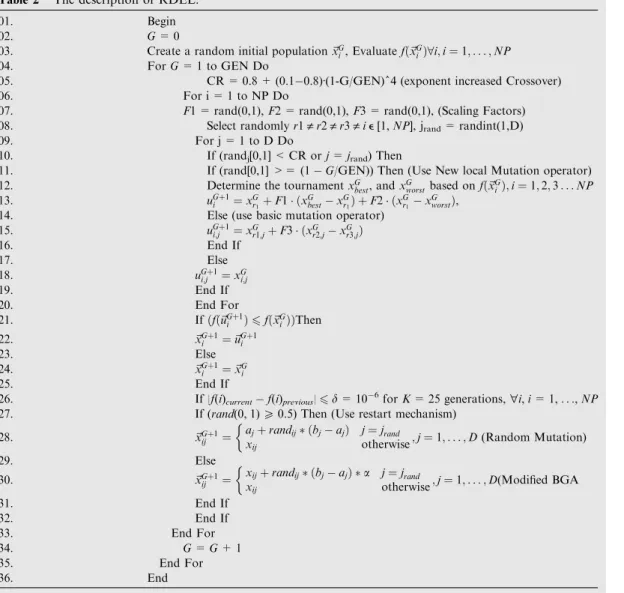
Table 2 The description of RDEL.
01. Begin
02. G= 0
03. Create a random initial population~xG
i, Evaluatefð~xGiÞ8i;i¼1;. . .;NP
04. ForG= 1 to GEN Do
05. CR = 0.8 + (0.10.8)Æ(1-G/GEN)^4 (exponent increased Crossover)
06. For i = 1 to NP Do
07. F1 = rand(0,1),F2 = rand(0,1),F3 = rand(0,1), (Scaling Factors) 08. Select randomlyr1„r2„r3„ie[1,NP], jrand= randint(1,D)
09. For j = 1 to D Do
10. If (randj[0,1] < CR orj=jrand) Then
11. If (rand[0,1] >= (1G/GEN)) Then (Use New local Mutation operator)
12. Determine the tournamentxG
best, andxGworstbased onfð~xiGÞ;i¼1;2;3. . .NP
13. uGþ1 i ¼xGr1þF1 ðx G bestxGr1Þ þF2 ðx G r1x G worstÞ,
14. Else (use basic mutation operator)
15. uGþ1 i;j ¼xGr1;jþF3 ðxGr2;jxGr3;jÞ 16. End If 17. Else 18. uGþ1 i;j ¼xGi;j 19. End If 20. End For 21. Ifðfð~uGþ1 i Þ6fð~xGiÞÞThen 22. ~xGþ1 i ¼~uGiþ1 23. Else 24. ~xGþ1 i ¼~xGi 25. End If 26. If |f(i)currentf(i)previous|6d= 10 6 forK= 25 generations,"i,i= 1,. . .,NP 27. If (rand(0, 1)P0.5) Then (Use restart mechanism)
28. ~xGþ1 ij ¼ ajþrandij ðbjajÞ j¼jrand xij otherwise ;j¼1;. . .;D(Random Mutation) 29. Else 30. ~xGþ1 ij ¼ xijþrandij ðbjajÞ a j¼jrand xij otherwise ;j¼1;. . .;D(Modified BGA 31. End If 32. End If 33. End For 34. G=G+ 1 35. End For 36. End
Therefore,Crshould take a small value in order to avoid the exceeding level of diversity that may result in premature convergence and slow convergence rate. Then, through generations, the variance of the population will decrease as the vectors in the population become similar. Thus, in order to advance diversity and increase the convergence speed, Cr should be a large value. Based on the above analysis and dis-cussion, and in order to balance between the diversity and the convergence rate or between global exploration ability and local exploitation tendency, a dynamic non-linear increased crossover probability scheme is proposed as follows:
Cr¼Crmaxþ ðCrminCrmaxÞ ð1G=GENÞ
k
ð15Þ
whereGis the current generation number,GENis the maxi-mum number of generations,CrminandCrmaxdenote the min-imum and maxmin-imum value of theCr, respectively, andkis a positive number. The optimal settings for these parameters areCrmin= 0.1,Crmax= 0.8 andk= 4. The algorithm starts atG= 0 withCrmin= 0.1 but asGincreases towardGEN, the Crincreases to reachCrmax= 0.8. As can be seen from Eq. (15),Crmin= 0.1 is considered as a good initial rate in order to avoid high level of diversity in the early stage as discussed earlier and by Storn and Price[2]. Additionally,Crmax= 0.8 is the maximum value of crossover that can balance between exploration and exploitation.k is set to its mean value as it is observed, if it is approximately less than or equal to 1 or 2 then the diversity of the population deteriorates for some func-tions and it could cause stagnation. On the other hand, if it is nearly greater than 6 or 7 it could cause premature conver-gence as the diversity sharply increases. The mean value of 4 was thus selected for all dimensions as the default value with all benchmark problems. A detailed description of RDEL is given inTable 2.
4. Experiments and discussion 4.1. Benchmark functions
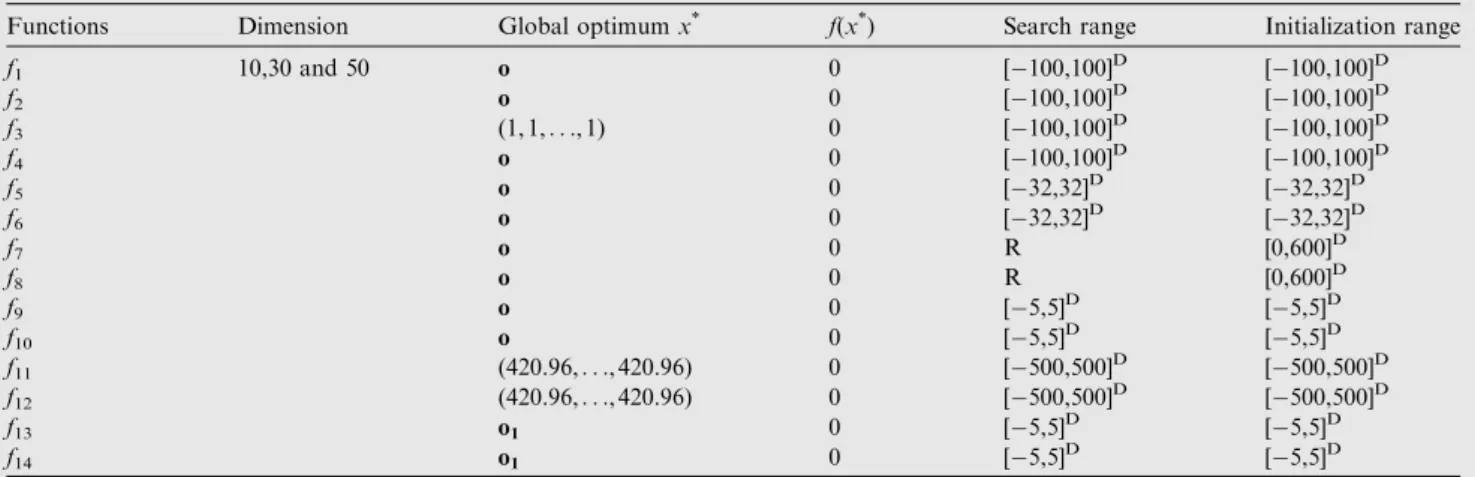
In order to evaluate the performance of the proposed algo-rithm (RDEL), 14 well-known benchmark test functions men-tioned in[5,35]are used. All these functions are minimization problems. Among the functions, f1–f4 are unimodal and
functions f5–f14 are multimodal. However, the generalized Rosenbrock’s function f3 is a multimodal function when D> 3[36]. These 14 test functions are dimension wise scal-able. Definitions of the Benchmark Problems are presented in Appendix A. The initialization ranges, the range of the search space, and the position of the global minimum for these 14 benchmark functions are presented inTable 3.
4.2. Algorithms for comparisons
In order to evaluate the benefits of the proposed modifications, a comparison of RDEL with six state-of-the-art self-adaptive differential evolution algorithms is made. These approaches are SaDE[15], jDE [9], ADE[14], JADE [16], SDE [13]and EPSDE[17]. The above benchmark functionsf1tof14are tested in 10-dimensions (10-D), 30-dimensions (30-D) and 50-dimen-sions (50-D).The maximum number of function evaluations is set to 100,00 for 10D problems, 300,000 for 30D problems and 500,000 for 50D problems. The population size is set to 50 for all dimensions with all functions. For each problem, 30 independent runs are performed and statistical results are pro-vided including the mean and the standard deviation values. The performance of different algorithms is statistically com-pared with RDEL by statisticalt-test with significance level of 0.05. Numerical values 1, 0, 1 (hvalues) represent that the RDEL is inferior to, equal to and superior to the algorithm with which it is compared, respectively. The experiments were car-ried out on an Intel (R) core i7 processor 1.6 GHz and 4 GB-RAM. RDEL algorithm is coded and realized in MATLAB. 4.3. Experimental results and discussions
The results (mean, standard deviation of the best-of-run errors and t-test results) of the comparisons are provided inTable 4 for 10-dimensions problems,Table 5for 30-dimensions prob-lems and Table 6for 50-dimensions problems. Note that the best-of-the-run error corresponds to absolute difference between the best-of-the-run valuefð~xbestÞand the actual
opti-mum f* of a particular objective function i.e. jfð~xbestÞ fj. The results provided by these approaches were directly taken from Ref.[17]. InTables 4–6, results are compared in terms of mean error and standard deviation. From the results, it
Table 3 Global optimum, search ranges and initialization ranges of the test functions.
Functions Dimension Global optimumx* f(x*) Search range Initialization range
f1 10,30 and 50 o 0 [100,100] D [100,100]D f2 o 0 [100,100]D [100,100]D f3 (1, 1,. . ., 1) 0 [100,100]D [100,100]D f4 o 0 [100,100]D [100,100]D f5 o 0 [32,32]D [32,32]D f6 o 0 [32,32]D [32,32]D f7 o 0 R [0,600]D f8 o 0 R [0,600]D f9 o 0 [5,5]D [5,5]D f10 o 0 [5,5]D [5,5]D f11 (420.96,. . ., 420.96) 0 [500,500]D [500,500]D f12 (420.96,. . ., 420.96) 0 [500,500]D [500,500]D f13 o1 0 [5,5] D [5,5]D f14 o1 0 [5,5] D [5,5]D ois the shifted vector.o1is the shifted vector for the first basic function in the composition function.
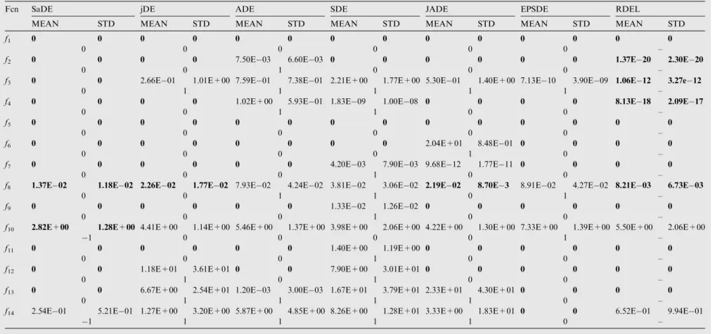
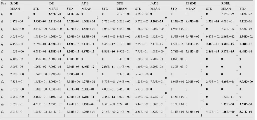
Table 4 Comparison between RDEL and various state-of-the-art methods on 10D problems.
Fcn SaDE jDE ADE SDE JADE EPSDE RDEL
MEAN STD MEAN STD MEAN STD MEAN STD MEAN STD MEAN STD MEAN STD
f1 0 0 0 0 0 0 0 0 0 0 0 0 0 0
0 0 0 0 0 0 –
f2 0 0 0 0 7.50E03 6.60E03 0 0 0 0 0 0 1.37E20 2.30E20
0 0 1 0 0 0 –
f3 0 0 2.66E01 1.01E+00 7.59E01 7.38E01 2.21E+00 1.77E+00 5.30E01 1.40E+00 7.13E10 3.90E09 1.06E12 3.27e12
0 1 1 1 1 1 –
f4 0 0 0 0 1.02E+00 5.93E01 1.83E09 1.00E08 0 0 0 0 8.13E18 2.09E17
0 0 1 1 0 0 –
f5 0 0 0 0 0 0 0 0 0 0 0 0 0 0
0 0 0 0 0 0 –
f6 0 0 0 0 0 0 0 0 2.04E+01 8.48E01 0 0 0 0
0 0 0 0 1 0 –
f7 0 0 0 0 0 0 4.20E03 7.90E03 9.68E12 1.77E11 0 0 0 0
0 0 0 1 0 0 –
f8 1.37E02 1.18E02 2.26E02 1.77E02 7.93E02 4.24E02 3.81E02 3.06E02 2.19E02 8.70E3 8.91E02 4.27E02 8.21E03 6.73E03
0 0 1 1 0 1 –
f9 0 0 0 0 0 0 1.33E02 1.26E02 0 0 0 0 0 0
0 0 0 1 0 0 –
f10 2.82E+00 1.28E+00 4.41E+00 1.14E+00 5.46E+00 1.37E+00 3.98E+00 2.06E+00 4.22E+00 1.30E+00 7.33E+00 1.39E+00 5.50E+00 2.06E+00
1 0 0 0 0 1 –
f11 0 0 0 0 0 0 1.40E+00 1.19E+00 0 0 0 0 0 0
0 0 0 1 0 0 –
f12 0 0 1.18E+01 3.61E+01 0 0 7.90E+00 3.01E+01 0 0 0 0 0 0
0 1 0 1 0 0 –
f13 0 0 6.67E+00 2.54E+01 1.20E03 3.00E03 1.67E+01 3.79E+01 2.33E+01 4.30E+01 0 0 0 0
0 1 1 1 1 0 –
f14 2.54E01 5.21E01 1.27E+00 3.20E+00 5.87E+00 4.85E+00 8.26E+00 1.28E+01 3.33E+00 1.83E+01 0 0 6.52E01 9.94E01
1 1 1 1 1 0 – Restart Differential Evolution algorithm based on Local Search Mutation for global numerical optimization: RDEL 181
Table 5 Comparison between RDEL and various state-of-the-art methods on 30D problems.
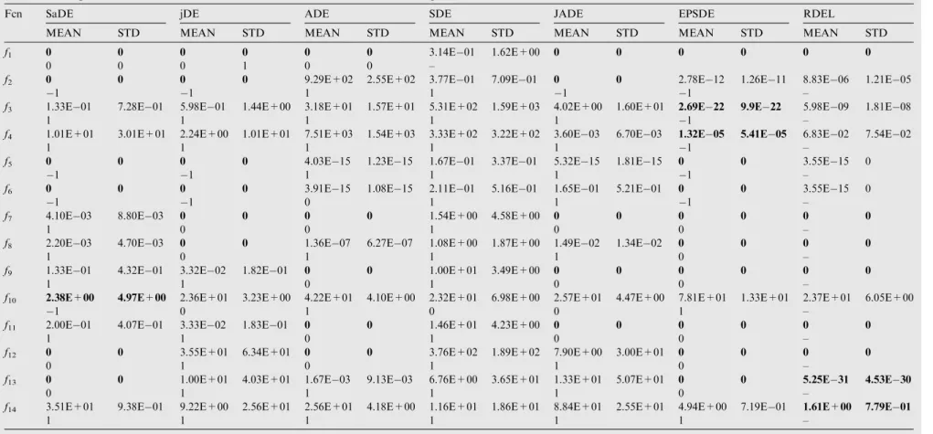
Fcn SaDE jDE ADE SDE JADE EPSDE RDEL
MEAN STD MEAN STD MEAN STD MEAN STD MEAN STD MEAN STD MEAN STD
f1 0 0 0 0 0 0 3.14E01 1.62E+00 0 0 0 0 0 0
0 0 0 1 0 0 –
f2 0 0 0 0 9.29E+02 2.55E+02 3.77E01 7.09E01 0 0 2.78E12 1.26E11 8.83E06 1.21E05
1 1 1 1 1 1 –
f3 1.33E01 7.28E01 5.98E01 1.44E+00 3.18E+01 1.57E+01 5.31E+02 1.59E+03 4.02E+00 1.60E+01 2.69E22 9.9E22 5.98E09 1.81E08
1 1 1 1 1 1 –
f4 1.01E+01 3.01E+01 2.24E+00 1.01E+01 7.51E+03 1.54E+03 3.33E+02 3.22E+02 3.60E03 6.70E03 1.32E05 5.41E05 6.83E02 7.54E02
1 1 1 1 1 1 –
f5 0 0 0 0 4.03E15 1.23E15 1.67E01 3.37E01 5.32E15 1.81E15 0 0 3.55E15 0
1 1 1 1 1 1 –
f6 0 0 0 0 3.91E15 1.08E15 2.11E01 5.16E01 1.65E01 5.21E01 0 0 3.55E15 0
1 1 0 1 1 1 –
f7 4.10E03 8.80E03 0 0 0 0 1.54E+00 4.58E+00 0 0 0 0 0 0
1 0 0 1 0 0 –
f8 2.20E03 4.70E03 0 0 1.36E07 6.27E07 1.08E+00 1.87E+00 1.49E02 1.34E02 0 0 0 0
1 0 1 1 1 0 –
f9 1.33E01 4.32E01 3.32E02 1.82E01 0 0 1.00E+01 3.49E+00 0 0 0 0 0 0
1 1 0 1 0 0 –
f10 2.38E+00 4.97E+00 2.36E+01 3.23E+00 4.22E+01 4.10E+00 2.32E+01 6.98E+00 2.57E+01 4.47E+00 7.81E+01 1.33E+01 2.37E+01 6.05E+00
1 0 1 0 0 1 –
f11 2.00E01 4.07E01 3.33E02 1.83E01 0 0 1.46E+01 4.23E+00 0 0 0 0 0 0
1 1 0 1 0 0 –
f12 0 0 3.55E+01 6.34E+01 0 0 3.76E+02 1.89E+02 7.90E+00 3.00E+01 0 0 0 0
0 1 0 1 1 0 –
f13 0 0 1.00E+01 4.03E+01 1.67E03 9.13E03 6.76E+00 3.65E+01 1.33E+01 5.07E+01 0 0 5.25E31 4.53E30
0 1 1 1 1 0 –
f14 3.51E+01 9.38E01 9.22E+00 2.56E+01 2.56E+01 4.18E+00 1.16E+01 1.86E+01 8.84E+01 2.55E+01 4.94E+00 7.19E01 1.61E+00 7.79E01
1 1 1 1 1 1 –
182
A.W.
Table 6 Comparison between RDEL and various state-of-the-art methods on 50D problems.
Fcn SaDE jDE ADE SDE JADE EPSDE RDEL
MEAN STD MEAN STD MEAN STD MEAN STD MEAN STD MEAN STD MEAN STD
f1 0 0 2.57E29 6.61E29 0 0 2.17E+01 3.85E+01 0 0 0 0 7.79E29 1.12E28
0 0 0 1 0 0 –
f2 1.47E09 5.93E09 2.11E04 2.72E04 1.70E+04 2.72E+03 3.26E+02 3.57E+02 5.20E23 1.13E22 4.47E09 1.75E08 4.58E01 5.12E01
1 1 1 1 1 1 –
f3 1.42E+00 2.44E+00 7.25E+00 1.77E+01 4.55E+01 1.08E+00 5.54E+06 1.36E+07 1.20E+00 1.93E+00 0 0 7.93E06 2.82E05
1 1 1 1 1 1 –
f4 3.05E+03 1.98E+03 1.26E+03 1.39E+03 4.15E+04 4.98E+03 9.46E+03 3.38E+03 1.42E+03 1.55E+03 5.47E+02 9.47E+02 2.66E+02 2.34E+02
1 1 1 1 1 1 –
f5 6.45E01 7.09E01 4.62E15 1.63E15 7.11E11 8.45E12 1.17E+00 7.35E01 7.11E15 1.52E16 8.05E15 2.46E15 3.90E15 1.08E15
1 0 1 1 0 0 –
f6 1.05E+00 6.58E01 4.38E15 1.50E15 6.87E15 8.86E16 9.90E01 7.95E01 1.08E+00 7.78E01 7.11E15 2.46E15 3.67E15 6.48E16
1 0 0 1 1 0 –
f7 6.40E03 1.15E02 2.00E04 1.30E03 0 0 1.40E+01 1.20E+01 5.70E03 1.09E01 0 0 0 0
1 1 0 1 1 0 –
f8 5.00E03 1.26E02 7.00E04 2.90E03 6.49E12 2.56E11 1.14E+01 1.40E+01 3.20E03 5.30E03 0 0 0 0
1 1 0 1 1 0 –
f9 2.09E+00 1.34E+00 1.99E01 3.99E01 0 0 2.39E+01 5.54E+00 0 0 0 0 0 0
1 1 0 1 0 0 –
f10 7.33E+01 1.65E+01 4.09E+01 5.98E+00 1.27E+02 9.79E+01 5.94E+01 1.23E+01 7.75E+01 1.96E+01 2.00E+02 2.90E+01 4.40E+01 9.03E+00
1 1 1 1 1 1 –
f11 1.57E+00 1.28E+00 3.33E01 4.71E01 2.00E01 4.00E01 3.46E+01 5.71E+00 0 0 0 0 0 0
1 1 1 1 0 0 –
f12 3.95E+00 2.16E+01 1.10E+02 1.36E+02 1.28E11 3.45E12 1.07E+03 3.29E+02 5.92E+01 1.15E+02 0 0 1.82E11 0
1 1 1 1 1 1 –
f13 1.67E+01 4.61E+01 2.33E+01 4.96E+01 1.19E08 6.52E08 2.24+01 5.44E+01 1.00E+01 3.16E+01 0 0 1.72E30 3.55E30
1 1 1 1 1 0 –
f14 5.01E+01 1.75E+02 2.41E+01 4.02E+01 1.26E+01 2.16E+00 2.14E+01 2.55E+01 1.52E+01 3.11E+01 3.15E+01 4.13E+01 1.15E+00 3.71E01
1 1 1 1 1 1 0 Restart Differential Evolution algorithm based on Local Search Mutation for global numerical optimization: RDEL 183
can be clearly concluded that RDEL can perform better than other compared algorithms in most of the cases. FromTable 4, it can be obviously seen that RDEL, SaDE and EPSDE exhibit better high quality results for all benchmark problems than jDE, ADE, SDE and JADE. From thet-test results, it can be observed that RDEL is inferior to, equal to, superior to compared algorithms in 2, 53 and 19 cases, respectively out of the total 84 cases. Thus, the RDEL is always either better or equal.Table 5indicates that the RDEL algorithm is supe-rior to the SDE algorithm in all functions in terms of average and Standard deviation values. However, RDEL is surpassed by the SDE algorithm on functionf10. Generally, the perfor-mance of RDEL algorithm is superior in most of the cases to SaDE, jDE, ADE and JADE algorithms, respectively. Finally, it can be observed that the performance of the RDEL and EPSDE algorithms are almost the same and they approx-imately achieved the same results in most of the functions. All in all, from the t-test results, it can be observed that RDEL is inferior to, equal to, superior to compared algorithms in 3, 44 and 41 cases, respectively out of the total 84 cases. Thus, the RDEL is almost either better or equal. According toTable 6, as the dimensionality of the problems increases from 10D to 50D, we can conclude that the performance of all other com-pared algorithms except RDEL and EPSDE deteriorates sig-nificantly. Therefore, it can be deduced that RDEL is superior to all algorithms and is competitive with EPSDE with high quality final solution with lower mean and standard devi-ation values. Moreover, the results show that the proposed RDEL algorithm outperforms EPSDE algorithm on the most difficult functions f4, f10 and f14 by remarkable difference.
From thet-test results, it is obvious that the RDEL are inferior to, equal to, superior to compared algorithms in 6, 22 and 56 cases, respectively out of the total 84 cases. Thus, the RDEL is almost either better or equal. In summary, our proposed RDEL approach can achieve better performance than all other competitive algorithms in terms of both the quality of the final solutions and robustness.
4.4. A parametric study on RDEL
In this section, in order to investigate the impact of the pro-posed modifications, some experiments are conducted. Two different versions of RDEL and conventional DE algorithm have been tested and compared against the proposed one.
1. Version 1: local mutation strategy is used without both the basic mutation scheme and the random and modified (BGA) mutations. (Denoted as RDEL-1.)
2. Version 2: local mutation strategy is combined with ran-dom and modified (BGA) mutations without using the basic mutation strategy. (Denoted as RDEL-2.)
3. Conventional DE: To investigate the gained advancement over the standard DE algorithm. DE/rand/1/bin strategy with (F= 0.5, CR= 0.9) is considered for comparison. These parameter settings are extensively used in the litera-ture[1,7,9]. (Denoted as DE.)
In order to evaluate the final solution quality, efficiency, convergence rate, and robustness produced by all algorithms, the performance of the two different versions of RDEL and
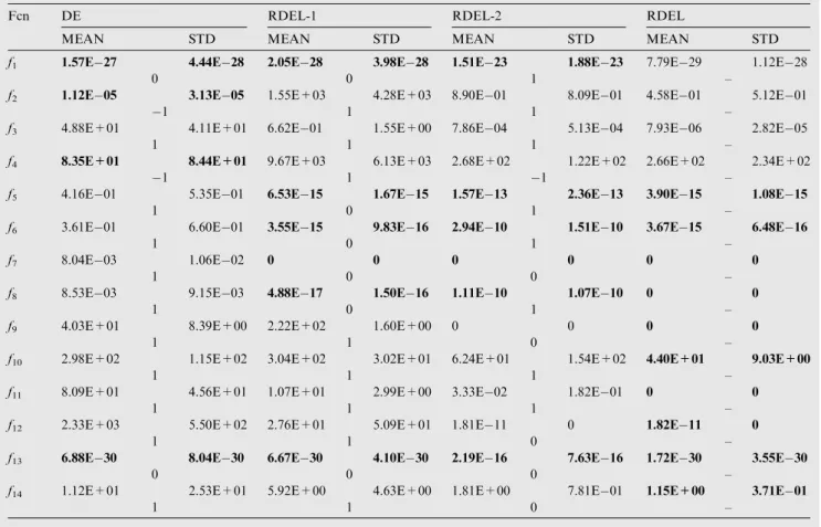
Table 7 Comparison between RDEL and RDEL with different versions and Basic DE on 50D problems.
Fcn DE RDEL-1 RDEL-2 RDEL
MEAN STD MEAN STD MEAN STD MEAN STD
f1 1.57E27 4.44E28 2.05E28 3.98E28 1.51E23 1.88E23 7.79E29 1.12E28
0 0 1 –
f2 1.12E05 3.13E05 1.55E+03 4.28E+03 8.90E01 8.09E01 4.58E01 5.12E01
1 1 1 –
f3 4.88E+01 4.11E+01 6.62E01 1.55E+00 7.86E04 5.13E04 7.93E06 2.82E05
1 1 1 –
f4 8.35E+01 8.44E+01 9.67E+03 6.13E+03 2.68E+02 1.22E+02 2.66E+02 2.34E+02
1 1 1 –
f5 4.16E01 5.35E01 6.53E15 1.67E15 1.57E13 2.36E13 3.90E15 1.08E15
1 0 1 –
f6 3.61E01 6.60E01 3.55E15 9.83E16 2.94E10 1.51E10 3.67E15 6.48E16
1 0 1 –
f7 8.04E03 1.06E02 0 0 0 0 0 0
1 0 0 –
f8 8.53E03 9.15E03 4.88E17 1.50E16 1.11E10 1.07E10 0 0
1 0 1 –
f9 4.03E+01 8.39E+00 2.22E+02 1.60E+00 0 0 0 0
1 1 0 –
f10 2.98E+02 1.15E+02 3.04E+02 3.02E+01 6.24E+01 1.54E+02 4.40E+01 9.03E+00
1 1 1 –
f11 8.09E+01 4.56E+01 1.07E+01 2.99E+00 3.33E02 1.82E01 0 0
1 1 1 –
f12 2.33E+03 5.50E+02 2.76E+01 5.09E+01 1.81E11 0 1.82E11 0
1 1 0 –
f13 6.88E30 8.04E30 6.67E30 4.10E30 2.19E16 7.63E16 1.72E30 3.55E30
0 0 0 –
f14 1.12E+01 2.53E+01 5.92E+00 4.63E+00 1.81E+00 7.81E01 1.15E+00 3.71E01
1 1 0 –
conventional DE algorithm are investigated based on the 50-dimensional functions. The parameters used are fixed as same as those in Section 4.2.
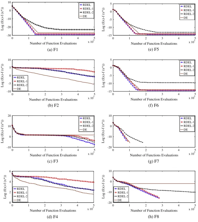
The overall comparison results of the RDEL algorithm against its versions and conventional DE algorithm are sum-marized inTable 7. Furthermore, in order to analyze the con-vergence behavior of each algorithm compared, the convergence characteristics in terms of the best fitness value of the median run of each algorithm for selected functions f3,f4,f6,f8,f10,f12andf13–f14with dimension 50 is illustrated inFig. 1. Indeed, the presented results inTable 7explain that the conventional DE only obtains better results on unimodal functions f1, f2, f4 and composition function f13 while it
completely fails on all multi-modal problems. Obviously, from the t-test results, it can be detected that RDEL is inferior to, equal to, superior to DE/rand/1/bin (F= 0.5, Cr= 0.9) in 2, 2 and 10 problems, respectively. Thus, the RDEL is much more efficient, robust and effective than DE/rand/1/bin (F= 0.5, Cr= 0.9) in finding high quality solution for real parameter optimization problems with dimensions 50. Accord-ingly, it can be deduced that the superiority, efficiency and the remarkable performance of the RDEL algorithm is due to the proposed modifications. On the other hand, concretely, it can be seen that the RDEL-1 algorithm significantly outperforms the conventional DE algorithm on functions (f3,f5–f8,f11,f12 and f14). Thus, it is worth mentioning that the RDEL-1
(a) F1 (b) F2 (c) F3 0 1 2 3 4 5 x 10⁵ -30 -20 -10 0 10
Number of Function Evaluations
Lo g (f(x )-f (x * )) RDEL RDEL-1 RDEL-2 DE 0 1 2 3 4 5 x 10⁵ -10 -5 0 5 10
Number of Functions Evaluations
Lo g (f(x )-f (x * )) RDEL RDEL-1 RDEL-2 DE 0 1 2 3 4 5 x 10⁵ -10 0 10 20
Number of Function Evaluations
Lo g (f(x )-f (x * )) RDELRDEL-1 RDEL-2 DE (d) F4 (e) F5 (f) F6 0 1 2 3 4 5 x 10⁵ 0 2 4 6
Number of Function Evaluations
Log (f(x)-f (x*)) RDEL RDEL-1 RDEL-2 DE 0 1 2 3 4 5 x 10⁵ -15 -10 -5 0 5
Number of Function Evaluations
Log (f(x)-f (x*)) RDEL RDEL-1 RDEL-2 DE 0 1 2 3 4 5 x 10⁵ -15 -10 -5 0 5
Number of Function Evaluations
Log (f(x)-f (x*)) RDEL RDEL-1 RDEL-2 DE (h) F8 0 1 2 3 4 5 x 10⁵ -20 -10 0 10
Number of Function Evaluations
Log (f(x)-f (x*)) RDEL RDEL-1 RDEL-2 DE (g) F7 0 1 2 3 4 5 x 10⁵ -20 -10 0 10
Number of Functions Evaluations
Lo g (f(x )-f (x * )) RDELRDEL-1 RDEL-2 DE
Figure 1 Convergence graph (median curves) of RDEL, RDEL-1, RDEL-2 and DE on 50-dimensional test functionsf1–f14. Restart Differential Evolution algorithm based on Local Search Mutation for global numerical optimization: RDEL 185
algorithm considerably improves the final solution quality. On the contrary, conventional DE algorithm has performed better than RDEL-1 on problem (f2,f4,f9andf10). Besides, they exhi-bit equal performance on 2 functions (f1andf13). Therefore, it is clearly observed that the proposed local mutation scheme with the proposed increased exponent crossover rule consider-ably balances the global exploration ability and local exploita-tion tendency for the majority of funcexploita-tions with different characteristics much more than standard DE algorithm, namely, DE/rand/1/bin strategy with (F= 0.5, Cr= 0.9). Indeed, from the t-test results, RDEL is inferior to, equal to, superior to RDEL-1 algorithm in 0, 6 and 8 problems, respec-tively. On the other hand, it can be seen that by embedding the random mutation and modified (BGA) mutation in RDEL-1 algorithm, extreme and ultimate improvement in the perfor-mance of RDEL-2 has been detected and achieved on func-tions (f2–f4, f9–f12 and f14). However, the joining of the random mutation and modified (BGA) mutation in RDEL-1 algorithm has a slight negative influence on the final solution quality and the convergence speed of RDEL-2 algorithm on functions (f1,f5–f8). Thus, from the t-test results, it can be observed that RDEL is inferior to, equal to, superior to RDEl-2 algorithm in 0, 9 and 5 problems, respectively. Conse-quently, RDEL algorithm is always either better or equal. Overall, it can be concluded that the excellent performance of the RDEL depends on the integration between its
compo-nents and it is superior to conventional DE, RDEL-1, RDEL-2. Additionally, the convergence graph inFig. 1, illus-trates that RDEL, RDEL-1 and RDEL-2 algorithms converge to better or global solution faster than conventional DE, in presented cases with exception to functionf4where basic DE converges faster than all compared algorithms. Accordingly, the main benefits of the proposed modifications are the remarkable balance between the exploration capability and exploitation tendency through the optimization process that leads to superior performance with fast convergence speed and the extreme robustness over the entire range of benchmark functions which are the weak points of all evolutionary algorithms.
5. Conclusion and future work
In order to promote the exploitation capability and speed up the convergence during the evolutionary process of the conven-tional DE algorithm, a restart Differential Evolution algo-rithm with novel local search mutation strategy for solving global numerical optimization problems over continuous space is proposed in this paper. Inspired by PSO algorithm, the pro-posed algorithm introduces a novel local mutation rule based on the position of the best and the worst individuals among the entire population of a particular generation. The mutation rule is combined with the basic mutation strategy through a (i) F9 0 1 2 3 4 5 x 10⁵ -15 -10 -5 0 5
Number of Function Evaluations
Log (f(x)-f (x*)) RDEL RDEL-1 RDEL-2 DE (j) F10 (k) F11 (l) F12 0 1 2 3 4 5 x 10⁵ 1.5 2 2.5 3 3.5
Number of Function Evaluations
Log (f(x)-f (x*)) RDEL RDEL-1 RDEL-2 DE 0 1 2 3 4 5 x 10⁵ -20 -10 0 10
Number of Function Evaluations
Log (f(x)-f (x*)) RDEL RDEL-1 RDEL-2 DE 0 1 2 3 4 5 x 10⁵ -15 -10 -5 0 5
Number of Function Evaluations
Lo g (f(x )-f (x * )) RDEL RDEL-1 RDEL-2 DE (m) F13 (n) F14 0 1 2 3 4 5 x 10⁵ -40 -20 0 20
Number of Function Evaluations
Lo g (f(x )-f (x * )) RDELRDEL-1 RDEL-2 DE 0 1 2 3 4 5 x 10⁵ -40 -20 0 20
Number of Function Evaluations
Lo g (f(x )-f (x * )) RDELRDEL-1 RDEL-2 DE Fig 1.(continued) 186 A.W. Mohamed
linear decreasing probability rule. The proposed mutation rule is shown to enhance the local search capabilities of the basic DE and to increase the convergence speed. Additionally, an exponent increased crossover probability rule is utilized to bal-ance the global exploration and local exploitation. Further-more, a random mutation scheme and a modified Breeder Genetic Algorithm (BGA) mutation scheme are merged to avoid stagnation and/or premature convergence. The proposed RDEL algorithm has been compared with 6 recent state-of-the-art parameter adaptive differential evolution variants over a suite of 14 bound constrained numerical optimization prob-lems. The experimental results and comparisons have shown that the RDEL algorithm performs better in unconstrained optimization problems with different types, complexity and dimensionality; it performs better with regard to the search process efficiency, the final solution quality, the convergence rate, and robustness, when compared with other algorithms. Current research efforts focus on applying the algorithm to solve high dimensions or large scale global optimization prob-lems as well as solving practical engineering optimization problems and real world applications. Finally, it would be very interesting to propose a self-adaptive RDEL version.
Appendix A
(1) Shifted sphere function
f1ðxÞ ¼
XD i¼1
z2
i;z¼xo;o¼ ½o1;o2;. . .;oD
:the shifted global optimum (2) Shifted Schwefel’s Problem 1.2
f2ðxÞ ¼ XD i¼1 mi j¼1zj 2 ;z¼xo;o¼ ½o1;o2;. . .;oD
:the shifted global optimum (3) Rosenbrock’s function f3ðxÞ ¼ XD1 i¼1 ð100ðx2 i xiþ1Þ 2 þ ðxi1Þ 2 Þ
(4) Shifted Schwefel’s Problem 1.2 with noise in fitness
f4ðxÞ ¼X D i¼1 ðX i j¼1 zjÞ 2 ð1þ0:4jNð0;1ÞjÞ;z¼xo;o
¼ ½o1;o2;. . .;oD:the shifted global optimum
(5) Shifted Ackley’s function
f5ðxÞ ¼ 20 exp 0:2 ffiffiffiffiffiffiffiffiffiffiffiffiffiffiffiffi 1 D XD i¼1 z2 i v u u t 0 @ 1 Aexp 1 D XD i¼1 cosð2pziÞ ! þ20þe;z
¼xo;o¼ ½o1;o2;. . .;oD:the shifted global optimum
(6) Shifted rotated Ackley’s function
f6ðxÞ ¼ 20 exp 0:2 ffiffiffiffiffiffiffiffiffiffiffiffiffiffiffiffi 1 D XD i¼1 z2 i v u u t 0 @ 1 Aexp 1 D XD i¼1 cosð2pziÞ ! þ20þe;z¼MðxoÞ;condðMÞ ¼1;o
¼ ½o1;o2;. . .;oD:the shifted global optimum
(7) Shifted Griewank’s function
f7ðxÞ ¼X D i¼1 z2 i 4000 YD i¼1 cos ziffiffi i p þ1;z¼xo;o
¼ ½o1;o2;. . .;oD:the shifted global optimum
(8) Shifted rotated Griewank’s function
f8ðxÞ ¼ XD i¼1 z2 i 4000 YD i¼1 cos ziffiffi i p þ1;z¼MðxoÞ; condðMÞ
¼3;o¼ ½o1;o2;. . .;oD:the shifted global optimum
(9) Shifted Rastrigin’s function
f9ðxÞ ¼
XD i¼1
ðz2
i 10 cosð2pziÞ þ10Þ;z¼xo;o
¼ ½o1;o2;. . .;oD:the shifted global optimum
(10) Shifted rotated Rastrigin’s function
f10ðxÞ ¼
XD i¼1
ðz2
i 10 cosð2pziÞ þ10Þ;z¼MðxoÞ; condðMÞ
¼2;o¼ ½o1;o2;. . .;oD:the shifted global optimum
(11) Shifted non-continuous Rastrigin’s function
f11ðxÞ ¼ XD i¼1 ðz2 i 10 cosð2pziÞ þ10Þ;yi ¼ zi jzij<1=2 roundð2ziÞ=2 jzijP1=2 ( fori¼1;2;. . .;D; z¼ ðxoÞ;
o¼ ½o1;o2;. . .;oD:the shifted global optimum
(12) Schwefel’s function f12ðxÞ ¼418:9829D XD i¼1 xisinðjxij 1=2 Þ (13) Composition function 1 (CF1) in[35]
The function f13(x) (CF1) is composed by using 10 sphere functions. The global optimum is easy to find once the global basin is found.
(14) Composition function 6 (CF6) in[35]
The functionf14(x) (CF6) is composed by using 10 dif-ferent benchmark functions, i.e. 2 rotated Rastrigin’s functions, 2 rotated Weierstrass functions, 2 rotated Griewank’s functions, 2 rotated Ackley’s functions and 2 rotated Sphere functions.
Where~oindicates the position of the shifted optima,M is a rotation matrix, and cond (M) is the condition number of the matrix.
References
[1] Storn R, Price K. Differential evolution – a simple and efficient adaptive scheme for global optimization over continuous spaces. Technical Report TR-95-012, ICSI; 1995. < http://.icsi.berke-ley.edu/~storn/litera.html>.
[2]Storn R, Price K. Differential evolution – a simple and efficient heuristic for global optimization over continuous spaces. J Global Optim 1997;11(4):341–59.
[3]Price K, Storn R, Lampinen J. Differential evolution: a practical approach to global optimization. Heidelberg: Springer; 2005. [4]Noman N, Iba H. Accelerating differential evolution using an
adaptive local search. IEEE Trans Evol Comput 2008;12(1): 107–25.
[5]Das S, Abraham A, Chakraborty UK, Konar A. Differential evolution using a neighborhood based mutation operator. IEEE Trans Evol Comput 2009;13(3):526–53.
[6] Lampinen J, Zelinka I. On stagnation of the differential evolution algorithm. In: Matousˇek R, Osˇmera P, editors. Proceedings of Mendel 2000, 6th international conference on soft computing; 2000. p. 76–83.
[7]Das SS, Suganthan PN. Differential evolution: a survey of the state-of-the-art. IEEE Trans Evol Comput 2011;15(1):4–31. [8] Xu Y, Wang L, Li L. An effective hybrid algorithm based on
simplex search and differential evolution for global optimization. In: International conference on intelligent computing; 2009. p. 341–50.
[9]Brest J, Greiner S, Bosˇkovic´ B, Mernik M, zˇumer V. Self-adapting control parameters in differential evolution: a comparative study on numerical benchmark problems. IEEE Trans Evol Comput 2006;10(6):646–57.
[10]Ga¨mperle R, Mu¨ller SD, Koumoutsakos P. A parameter study for differential evolution. In: Grmela A, Mastorakis NE, editors. Advances in intelligent systems, fuzzy systems, evolutionary computation. Interlaken, Switzerland: WSEAS Press; 2002. p. 293–8.
[11]Ro¨nkko¨nen J, Kukkonen S, Price KV. Real-parameter optimiza-tion with differential evoluoptimiza-tion. Proc IEEE cong evol comput, vol. 1. Washington, DC: IEEE Computer Society; 2005. p. 506–13. [12]Liu J, Lampinen J. A fuzzy adaptive differential evolution
algorithm. Soft Comput 2005;9(6):448–62.
[13] Omran MGH, Salman A, Engelbrecht AP. Self-adaptive differ-ential evolution, in: Computational intelligence and security, PT 1, proceedings lecture notes in artificial intelligence; 2005. p. 192–99. [14] Zaharie D. Control of population diversity and adaptation in differential evolution algorithms. In: Matousek R, Osmera P, editors. Proceedings of Mendel 2003, 9th international conference on soft computing; 2003, p. 41–6.
[15]Qin AK, Huang VL, Suganthan PN. Differential evolution algorithm with strategy adaptation for global numerical optimi-zation. IEEE Trans Evol Comput 2009;13(2):398–417.
[16]Zhang JQ, Sanderson AC. JADE: adaptive differential evolution with optional external archive. IEEE Trans Evol Comput 2009;13(5):945–58.
[17]Mallipeddi R, Suganthan PN, Pan QK, Tasgetiren MF. Differ-ential evolution algorithm with ensemble of parameters and mutation strategies. Appl Soft Comput 2011;11(2):1679–96.
[18] Fan HY, Lampinen J. A trigonometric mutation approach to differential evolution. J Global Optim 2003;27(1):105–29. [19] Das S, Konar A, Chakraborty UK. Two improved differential
evolution schemes for faster global search. In: GECCO ‘05 Proceedings of the 2005 conference on Genetic and evolutionary computation; 2005. p. 991–8.
[20] Kaelo P, Ali MM. A numerical study of some modified differ-ential evolution. Eur J Oper Res 2006;196(3):1176–84.
[21] Price KV. An introduction to differential evolution. In: Corne D, Dorgio M, Glover F, editors. New ideas in optimization. London, UK: McGraw-Hill; 1999. p. 79–108.
[22] Mohamed AW, Sabry HZ. Constrained optimization based on modified differential evolution algorithm. Inf Sci 2012;194: 171–208.
[23] Liu G, Li Y, Nie X, Zheng H. A novel clustering-based differential evolution with 2 multi-parent crossovers for global optimization. Appl Soft Comput 2012;12(2):663–81.
[24] Omran MGH, Engelbrecht AP, Salman A. Bare bones differential evolution. Eur J Oper Res 2009;196:128–39.
[25] Piotrowski AP, Napiorkowski JJ, Kiczko A. Differential evolu-tion algorithm with separated groups for multi-dimensional optimization problems. Eur J Oper Res 2012;216:33–46. [26] Mohamed AW, Sabry HZ, Abd-Elaziz T. Real parameter
optimization by an effective differential evolution algorithm. Egypt Inform J 2013;14:37–53.
[27] Ali M, Siarry P, Pant M. An efficient differential evolution based algorithm for solving multi-objective optimization problems. Eur J Oper Res 2012;2012(217):404–16.
[28] Islam SM, Das S, Ghosh S, Roy S, Suganthan PN. An adaptive differential evolution algorithm with novel mutation and cross-over strategies for global numerical optimization. IEEE Trans Syst Man Cybern Part B: Cybern 2012;42(2):482–500.
[29] Elsayed S, Sarker R, Essam D. Self-adaptive differential evolution incorporating a heuristic mixing of operators. Comput Optim Appl 2012:1–20.
[30] Elsayed S, Sarker R, Ray T. Parameters adaptation in differential evolution. In: IEEE congress on evolutionary computation, Brisbane; 2012b. p. 1–8.
[31] Triguero I, Derrac J, Garci S, Herrera F. Integrating a differential evolution feature weighting scheme into prototype generation. Neurocomputing 2012;97:332–43.
[32] Ali M, Pant M, Abraham A. Improving differential evolution algorithm by synergizing different improvement mechanisms. ACM Trans Auton Adapt Syst 2012;7(2):1–32.
[33] Mu¨hlenbein H, Voosen DS. Predictive models for the breeder genetic algorithm – I. Continuous parameter optimization. Evol Comput 1993;1(1):25–49.
[34] Feoktistov V. Differential evolution: in search of solutions. Berlin, Germany: Springer-verlag; 2006.
[35] Liang JJ, Suganthan PN, Deb K. Novel composition test functions for numerical global optimization. In: Proceedings of IEEE swarm intelligence symposium, Pasadena, CA; 2005. p. 68–75.
[36] Shang YW, Qiu YH. A note on the extended Rosenbrock function. Evol Comput 2006;14(1):119–26.