Aalto University School of Science
Degree Programme in Computer, Communication and Information Sciences
Yury Shukhrov
Lightweight Massively Parallel
Suffix Array Construction
Master’s Thesis Espoo, May 26, 2019
ABSTRACT OF MASTER’S THESIS Aalto University
School of Science
Degree Programme in Computer, Communication and Information Sciences Author: Yury Shukhrov
Title: Lightweight Massively Parallel Suffix Array Construction
Date: May 26, 2019 Pages: 88
Major: Computer Science Code: SCI3042
Supervisor: Professor Petteri Kaski
The suffix array is an array of sorted suffixes in lexicographic order, where each sorted suffix is represented by its starting position in the input string. It is a fundamental data structure that finds various applications in areas such as string processing, text indexing, data compression, computational biology, and many more. Over the last three decades, researchers have proposed a broad spectrum of suffix array construction algorithms (SACAs). However, the majority of SACAs were implemented using sequential and parallel programming models. The matu-rity of GPU programming opened doors to the development of massively parallel GPU SACAs that outperform the fastest versions of suffix sorting algorithms op-timized for the CPU parallel computing. Over the last five years, several GPU SACA approaches were proposed and implemented. They prioritized the running time over lightweight design.
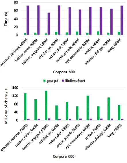
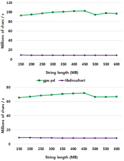
In this thesis, we design and implement a lightweight massively parallel SACA on the GPU using the prefix-doubling technique. Our prefix-doubling implementa-tion is memory-efficient and can successfully construct the suffix array for input strings as large as 640 megabytes (MB) on Tesla P100 GPU. On large datasets, our implementation achieves a speedup of 7-16x over the fastest, highly opti-mized, OpenMP-accelerated suffix array constructor,libdivsufsort, that leverages the CPU shared memory parallelism. The performance of our algorithm relies on several high-performance parallel primitives such as radix sort, conditional filtering, inclusive prefix sum, random memory scattering, and segmented sort. We evaluate the performance of our implementation over a variety of real-world datasets with respect to its runtime, throughput, memory usage, and scalability. We compare our results against libdivsufsort that we run on a Haswell compute node equipped with 24 cores. Our GPU SACA is simple and compact, consisting of less than 300 lines of readable and effective source code. Additionally, we de-sign and implement a fast and lightweight algorithm for checking the correctness of the suffix array.
Keywords: suffix array construction, GPU, prefix-doubling, CUDA, skew, Burrows-Wheeler transform, algorithm engineering, parallel primitives, induced sorting
Acknowledgements
First and foremost, I would like to express my sincere gratitude to my su-pervisor, Professor Petteri Kaski, for his continuous support, patience, and guidance throughout the course of this work. I also wish to thank him for pro-viding me the opportunity to work on a challenging yet exciting project. His constructive feedback, immense knowledge, and valuable suggestions have contributed greatly to the improvement of the thesis.
I would like to acknowledge the use of computing resources available via project ”Science-IT” at Aalto University School of Science and via CSC— the Finnish IT Center for Science. As regards the latter I would especially like to thank ”Science-IT” administrators for granting me access to the Triton cluster to carry out the experiments in this thesis.
Finally, I would like to thank my parents for their support and faith in my ability to attain my goals.
Espoo, May 26, 2019 Yury Shukhrov
Contents
1 Introduction 1
2 Background 4
2.1 Notation and Terminology . . . 4
2.2 The Suffix Array . . . 7
2.3 The Burrows-Wheeler Transform . . . 9
2.4 Prior Work . . . 11
3 Algorithms for Suffix Array Construction 15 3.1 Prefix-Doubling Algorithms . . . 16
3.1.1 Manber and Myers Algorithm . . . 16
3.1.2 Larsson and Sadakane Algorithm . . . 23
3.2 Recursive Algorithms . . . 28
3.3 Induced Sorting Algorithms . . . 30
4 GPU Parallel Programming 34 4.1 Compute Unified Device Architecture . . . 34
4.2 Essentials of the Thrust Library . . . 36
4.2.1 Host and Device Vectors . . . 37
4.2.2 Interoperability . . . 38
4.2.3 Anonymous Kernels . . . 40
4.3 Parallel Primitives . . . 42
4.3.1 Radix Sort . . . 42
4.3.2 Select-Flagged . . . 44
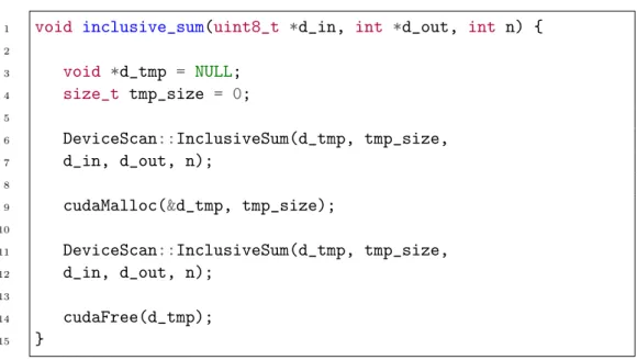
4.3.3 Inclusive Prefix Sum . . . 46
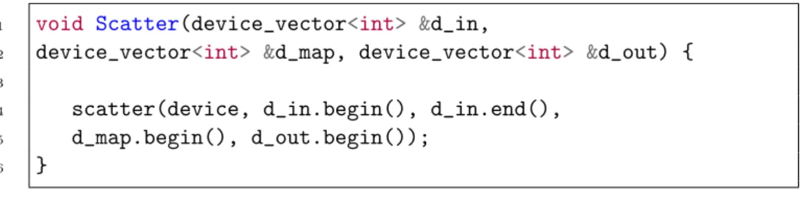
4.3.4 Scatter . . . 48
4.3.5 Segmented Sort . . . 49
5 Implementations 52 5.1 Choosing the Algorithm . . . 53
5.3 The Suffix Array Checker . . . 66 6 Experimental Results 69 6.1 Hardware Specifications . . . 69 6.2 Performance Evaluation . . . 70 6.3 Scalability Analysis . . . 74 7 Conclusions 77
Chapter 1
Introduction
The problem of suffix sorting boils down to finding a lexicographic order of all suffixes in a string. The suffix array (SA) is an elegant and compact data structure that stores the starting positions of sorted suffixes. The concept of the SA was proposed in 1990 by Manber and Myers [53] as the space-saving substitute of the suffix tree [19, 24] data structure. The SA finds an important application in different areas such as stringology [16], genome analysis [2], bioinformatics [18], and many more.
For example, one can use the SA to determine quickly if a given text contains a required pattern. Instead of constructing an index structure for the text by repetitive queries and text preprocessing, the SA provides an immediate index structure solution. Thus, to find all matches of a pattern in a text one needs to identify each suffix that begins with a pattern. A simple solution requires a double pass of a binary search [91] to locate the first and last index of the interval containing the pattern. This kind of indexes is called full-text indexes [50].
Another application of the SA is in data compression. The SA plays an important role inBurrows-Wheeler transformation (BWT) introduced by Burrows and Wheeler in 1994 [12]. The BWT of a string is obtained by generating cyclic rotations of this string, by sorting them in lexicographic order, and by extracting the last character of these sorted strings. This transformation is reversible with minimal data overhead. The BWT can be efficiently computed as a simple modification of the SA. It is a powerful tool for transforming data into a form suitable for lossless compression algorithms incorporated in popular compressors such as bzip2 [7] and szip [78].
A trivial way to construct the suffix array of the input text is to employ a sorting algorithm (e.g., quick sort ormerge sort [27, 41]) to find the lexico-graphic order of suffixes. This approach will result in O(n2logn) time com-plexity because O(nlogn) comparisons are used and each string comparison
takes O(n) time. However, we can significantly improve on that complexity if we utilize the knowledge that there is some dependency between suffixes. In fact, suffixes are overlapping substrings.
Currently, suffix array construction algorithms (SACAs) that take advan-tage of this knowledge can be classified into three main categories: prefix-doubling,recursive, andinduced sorting [74]. Prefix-doubling SACAs use the rank of prefixes to determine the order of suffixes, where the length of each prefix is doubled in each iteration. Recursive SACA approaches group suf-fixes into two subsets according to some criteria. One subset with 2/3 or less suffixes is recursively sorted, and its order is used to induce the order of the second subset. Once both subsets are sorted, merge sort is used to combine the results. Induced sorting algorithms use the information about the sorted subset of suffixes to induce the order of the remaining suffixes.
Over the past two decades, the majority of the proposed SACAs have been implemented using the sequential programming model. The advances and accessibility of the general-purpose computing on graphics cards (GPGPU) have spurred interest in designing an efficient SACA that would harness the power of massively parallel GPU architectures and outperform currently fastest parallel SACAs built for multi-core CPU architectures. In the past five years, there were several approaches to design and implement a shared mem-ory parallel SACA using the GPU programming model. The most prominent is the implementation of Deo and Kelly [17], based on the skew algorithm [77]; the implementation of Osipov [73], based on prefix-doubling method; and the implementation of Wang et al. [89], based on a hybrid skew prefix-doubling approach.
To best of our knowledge, previous approaches to constructing a suffix ar-ray with GPGPU coding prioritized the running time of the implementation over other technical aspects. As a result, implementations in the previous approaches lacked a simple, compact and lightweight design. We are mo-tivated to improve on the previous approaches in terms of simplicity and compactness of the GPU SACA implementation. In this thesis, we design and implement a lightweight and memory-efficient GPU SACA using modern, high-performance, state-of-the-art parallel primitives to achieve best results. We experimentally evaluate the performance of our implementation using real-world datasets and comparing the runtime, throughput, and scalabil-ity against the fastest in practice suffix sorting algorithm working in main memory [21], libdivsufsort [61].
This thesis is organized as follows: we begin in Chapter 2 with a brief introduction to the basic definitions and notations in stringology, we study basic properties of the SA and its inverse. Then, we describe the BTW and demonstrate how it can be efficiently constructed by the SA. Finally, we give
a short review of the prior work done in the area of suffix array construction. In Chapter 3, we discuss three fundamental methods for suffix array con-struction. We study working principles of the SACAs based on each method. In Chapter 4, we review the programming model for GPGPU: we begin with a brief introduction to Compute Unified Device Architecture (CUDA), then we cover essentials of the Thrust library that are employed in our imple-mentation, and explain the working principles of the most efficient parallel primitives that were incorporated in our GPU SACA implementation. In Chapter 5, we present our GPU SACA implementation and justify the rea-son for choosing the prefix-doubling method. Additionally, we present a fast and lightweight implementation of the suffix array checker. This program serves the purpose of checking the correctness of our GPU SACA implemen-tation. Its working principles are based on three conditions for checking the correctness of the suffix array. We discuss these conditions and describe our implementation approach. Experimental evaluation of our implementation and the corresponding results are presented in Chapter 6. We conclude this thesis in Chapter 7.
Chapter 2
Background
In this chapter, we give a brief introduction to basic terminologies and defi-nitions in stringology. We describe the concept of the suffix array data struc-ture and expose the related notation. We study the working principles of the Burrows-Wheeler Transform (BWT) and demonstrate how to efficiently con-struct a BWT string directly from the SA. The chapter ends with a review of the advances in suffix array construction.
2.1
Notation and Terminology
A string is a sequence of characters drawn from a finite set, called alphabet. The alphabet may contain symbols, letters or characters. We will usually denote an alphabet with the symbol Σ and its size with σ, that is |Σ| = σ. The size of the alphabet is the number of unique elements in it [15, 16]. Example 2.1. The most common type of the alphabet is the basic modern Latin alphabet of lowercase letters:
Σ ={a, b, c, . . . , x, y, z}.
This alphabets contains 26 distinct letters, that is σ = 26. The word S = abracadabra is an example of a string over the alphabet Σ.
Let Σ1 = {0,1} be the alphabet of size two containing binary numbers. Then strings ε,0,1,00,01,10,11,000, etc. are all in Σ1, where ε represents the empty string. This kind of alphabet is commonly used in the context of finite automata [82].
Other commonly used alphabets include the set of 256 8-bit ASCII ( (American Standard Code for Information Interchange) [49] symbols or the set of DNA (DeoxyriboNucleic Acid) characters [84].
We denote the set of all strings over an alphabet Σ by Σ∗ = ∞ [ t=0 Σt = Σ0∪Σ1∪Σ2 ∪. . . , where Σt= t z }| { Σ×Σ× · · · ×Σ ={x1x2. . . xt|xi ∈Σ for 1 ≤i≤t}
denotes the set of all strings on Σ having length t.
The length of a string x, denoted by |x|, is the number of alphabet el-ements it contains. Given a string x of length n, we denote by x[i], for i ∈ [0, n), the character of a string x at the position i or at index i of x assuming that we are dealing with azero-indexed string, that is a string with the first character positioned at index zero instead of one.
We can denote a string S of length n using either index separated by comma notation or index-range notation. In the first case, we mark the starting index and ending index of S separated by a comma. In the second case, we write the starting index and ending index of S separated by the range symbol.
Example 2.2. Given a string S of length n, we denote it as S =S[1, n] =S[1]S[2]. . . S[n] =S[1. . . n],
if it starts at index 1 and ends at index n. We can express zero-indexed strings T of lengthn as follows:
T =T[0, n−1] =T[0]T[1]. . . T[n−1] =T[0. . . n).
Given a string S[0, n) with n characters, S[i . . . j] ⊂ S denotes the sub-string of S that starts at position i and ends at position j, such that i ≤j. When i > j, S[i . . . j] denotes the empty string ε.
Example 2.3. Suppose we are given a string T[0,11] =abracadabra$. To define a substring bracawe provide its starting and ending character indices within the array T, that isT[1,4] = braca.
Let x be a string of length n and let y be a string of length m. The concatenation of x and y, denoted by xy, is the string formed by merging x and y, as in x1· · ·xny1. . . ym. We write xn to denote that string x is
concatenated with itself n times, that is, x0 =ε and xn=
n
z }| { xx· · ·x .
Example 2.4. Let x = abra and y = cadabra. The concatenation of x and y is xy =abracadabra. To obtain x2 we append x to the end of itself, that is, x2 =abraabra.
Given a string S[1. . . n] with n symbols, a substring S[i . . . n] ⊂ S is a suffix of S that starts at index i and ends at the end of S. A proper suffix of the string S is any suffix of S such that 1< i≤n, that is, any non-empty suffix of S that is not equal to S. A prefix of S is a substring S[1. . . i]⊂S that starts from the beginning of S and ends at index i. A proper prefix of the string S is any prefix of S such that 1 ≤ i < n, that is, any non-empty prefix of S that is not equal to S [51].
Example 2.5. Suffixes and prefixes of the string T =abracadabra$. Suffix Prefix Index
abracadabra$ a 0 bracadabra$ ab 1 racadabra$ abr 2 acadabra$ abra 3 cadabra$ abrac 4 adabra$ abraca 5 dabra$ abracad 6 abra$ abracada 7 bra$ abracadab 8 ra$ abracadabr 9 a$ abracadabra 10 $ abracadabra$ 11
In Example 2.5, you can see that a suffix of the stringT starts from the cor-responding index and includes all characters in between until and including the last character. Thus, if we consider suffix 5, adabra$, we can express it as T[5. . .11]. Observe that the prefix is reciprocal in some way to the suffix. Suffix index tells us that it starts from that index and spans over all characters until and including the last character. The same index tells us that the prefix is a substring that starts from the first index and ends on the suffix index. Hence, prefix 5,abraca can be defined as T[0. . .5].
Thelexicographic ordering, denoted by<, is a total ordering on the alpha-bet Σ that induces the ordering on Σ∗ as follows. Given two stringss, t ∈Σ∗, we say thats is lexicographically smaller thant, written ass < t, if and only if either s is a proper prefix oft or we can express the first string as s=xcy and the second string as t = xdz with x, y, z ∈ Σ∗ and characters c, d ∈ Σ such that c < d [15, 70].
Example 2.6. Suppose we have three strings: x=acacc, y=accaand z= accaac. To determine the lexicographic ordering of these strings we compare their first characters index-wise. Assume thata < c. The first two characters of all three strings are the same, so we need to look at the third character. We see that in string x this character is a which is smaller than in the other two strings that have character cat that index. This tells us that xis lexicographically the smallest among three strings. Next, we compare y and z. The first four characters are the same. However, we notice that y is a proper prefix of z. Hence the lexicographic ordering isx < y < z.
2.2
The Suffix Array
Let x[0. . . n] be a string of length n + 1 over an indexed alphabet Σ (i.e. an alphabet where each symbol is associated with an integer that belongs to some limited range). We assume that x[n] =$ is a special symbol called the sentinel that is usually marked with a dollar sign $ such that $ is lexi-cographically smaller than any other symbol in Σ [18].
We denote thei-th suffix ofxasxi =x[i . . . n] orsuffix i. Thesuffix array
of the string x, written as SAx or just SA, is an array of integers SA[0. . . n],
which stores a permutation of the integers {0, . . . , n}, such that xSA[0]< xSA[1] <· · ·< xSA[n].
To put it another way,xi is thej-th smallest suffix of the stringxin ascending
lexicographical order if and only if SA[j] =i [64].
Example 2.7. The suffix array of the string x=abracadabra$. Suffix i Sorted suffix SA[i]
abracadabra$ 0 $ 11 bracadabra$ 1 a$ 10 racadabra$ 2 abra$ 7 acadabra$ 3 abracadabra$ 0 cadabra$ 4 acadabra$ 3 adabra$ 5 adabra$ 5 dabra$ 6 bra$ 8 abra$ 7 bracadabra$ 1 bra$ 8 cadabra$ 4 ra$ 9 dabra$ 6 a$ 10 ra$ 9 $ 11 racadabra$ 2
Example 2.7 tells us thatx11is the 0-th smallest suffix,x10is the 1-th smallest suffix, and so on (assuming that we use zero-indexed string and lexicograph-ical order of the characters). Notice that |x| = |SA| and that SA is the permutation of the set {0, . . . ,11}.
The inverse suffix array of the string x, written as ISAx or just ISA, is
an array of integers ISA[0. . . n], so that for anyiwith 0≤i≤n the equality ISA[SA[i]] = i. More precisely, the relation between SA and ISA can be expressed as follows:
ISA[i] =j ⇔SA[j] =i.
The inverse suffix array is also called the lexicographic ranks of suffixes be-cause ISA[i] specifies the rank of the i-th suffix among the lexicographically ordered suffixes [74]. The expression ISA[i] = j implies that suffix xi is the
j-th smallest suffix of the stringxin ascending lexicographical order [51, 64]. We can compute SA and ISA, one from the other, in linear time as follows:
SA[ISA[i]] =i, 0≤i≤n and ISA[SA[j]] =j, 0≤j ≤n. Example 2.8. The suffix array and the inverse suffix array of the string x=abracadabra$.
Suffix i Sorted suffix SA[i] ISA[i]
abracadabra$ 0 $ 11 3 bracadabra$ 1 a$ 10 7 racadabra$ 2 abra$ 7 11 acadabra$ 3 abracadabra$ 0 4 cadabra$ 4 acadabra$ 3 8 adabra$ 5 adabra$ 5 5 dabra$ 6 bra$ 8 9 abra$ 7 bracadabra$ 1 2 bra$ 8 cadabra$ 4 6 ra$ 9 dabra$ 6 10 a$ 10 ra$ 9 1 $ 11 racadabra$ 2 0
Example 2.8 tells us thatx0 is the 3-th smallest suffix,x1 is the 7-th smallest suffix, and so on. To compute SA from ISA we take the following steps: SA[ISA[0]] = SA[3] = 0, SA[ISA[1]] = SA[7] = 1, and so on. To compute ISA from SA we take the following steps: ISA[SA[0]] = ISA[11] = 0, ISA[SA[1]] = ISA[10] = 1, and so on. Obviously, we can compute SA from ISA and vice versa in linear time.
2.3
The Burrows-Wheeler Transform
The Burrows-Wheeler Transform (BWT) [12] is a process of transforming an input string into another string that has a structure suitable for efficient compression. A remarkable property of this structure is that a string gener-ated by the BWT tends to contain a large number of substrings composed of consecutive identical characters. To take advantage of this property and effi-ciently code a string generated by the BWT, a Move-to-Front (MTF) [9, 76] and a Huffman [31, 87] or arithmetic [93] coders are used.
The BTW is reversible, which enables a recovery of the original string with minimal data overhead. The BWT of a string x[0. . . n] is generated as follows: (1) Append a sentinel symbol $ to the end of the string x such that x[n] = $ (2) Construct a n + 1×n + 1 matrix R containing all rotations (cyclic shifts) of x. (3) Sort rotations in R lexicographically. (4) The last column of R is the output of the BWT [12, 71].
Example 2.9. Application of the BWT with input stringx=abracadabra.
i Rotations (R) Sorted rotations BWT[i] 0 abracadabra$ $abracadabra a 1 bracadabra$a a$abracadabr r 2 racadabra$ab abra$abracad d 3 acadabra$abr abracadabra$ $ 4 cadabra$abra acadabra$abr r 5 adabra$abrac adabra$abrac c 6 dabra$abraca bra$abracada a 7 abra$abracad bracadabra$a a 8 bra$abracada cadabra$abra a 9 ra$abracadab dabra$abraca a 10 a$abracadabr ra$abracadab b 11 $abracadabra racadabra$ab b
Observe that when cyclic shifts are applied on the string abracadabra$, the sentinel symbol $ shifts from right to left until it reaches the first position in the last rotation. The output of the transformation is ard$rcaaaabb. Although the length of the input string is small, the structure of the output string contains substrings of consecutive identical characters, which are easy to compress using the coders mentioned at the beginning of this chapter. In practice, input strings of sufficiently large length are likely to generate
more substrings of consecutive identical characters, as a result of the BTW transformation, and hence the compression efficiency tends to increase.
The efficiency of the original approach for computing the BTW of a string boils down to the efficiency of sorting lexicographically the rotations of the Burrows-Wheeler Matrix (BWM). In other words, sorting the rotations is a bottleneck in the BWT with respect to the time complexity of this operation. A naive approach is to sort the rotations using a comparison-based sorting algorithm such asquicksort ormergesort. However, a more sophisticated and efficient approach is to employ the suffix array to solve the problem of sorting the rotations [3, 46].
Observe that the sorted rotations resemble the sorted suffixes obtained from the suffix array of the stringx=abracadabra$. We notice in Example 2.10 that each sorted rotation can be obtained by extracting a corresponding sorted suffix of xand prepending it to the beginning of x.
Example 2.10. The relation between the BWT and the SA with input string x=abracadabra$.
i Sorted rotations Sorted suffixes of x SA[i] BWT[i]
0 $abracadabra $ 11 a
1 a$abracadabr a$ 10 r
2 abra$abracad abra$ 7 d
3 abracadabra$ abracadabra$ 0 $
4 acadabra$abr acadabra$ 3 r
5 adabra$abrac adabra$ 5 c
6 bra$abracada bra$ 8 a
7 bracadabra$a bracadabra$ 1 a
8 cadabra$abra cadabra$ 4 a
9 dabra$abraca dabra$ 6 a
10 ra$abracadab ra$ 9 b
11 racadabra$ab racadabra$ 2 b
The relation between the BWT and the SA can be formulated as follows: BWT[i] =
(
x[SA[i]−1] if SA[i]>0 $ if SA[i] = 0
This relation implies that BWT[i] of the string x can be constructed by taking a character that is positioned to the left of the suffix in the suffix array SA[i].
2.4
Prior Work
In this section, we give a short review of the most notable SACAs and clas-sify them according to three categories: sequential implementations, parallel CPU implementations and massively parallel GPU implementations. The se-quential implementation class of algorithms includes all SACAs that run in a single thread and execute CPU instructions sequentially. A class of parallel CPU implementations includes SACAs that leverage multi-core CPU par-allelism and shared-memory data access. These are multi-threaded SACAs that can be powered by some application programming interface (API) that supports multi-platform shared memory multiprocessing programming. Fi-nally, the last class includes SACAs developed for massively parallel shared-memory GPU architectures.
Sequential Implementations
The concept of the suffix array was introduced in 1990 by Manber and Myers (MM) [53] along with the firstO(nlogn) [47] suffix sorting algorithm, which consumed less space than alternative suffix tree implementations. Their work was motivated by the results of Karp et al. in 1972 [38] who was working on pattern matching in strings using array and tree data structures. The MM algorithm was later improved and optimized by Larsson and Sadakane (LS) [45]. Both the MM and the LS algorithms used prefix-doubling tech-nique. According to [74], the LS algorithm was ten times faster than the MM algorithm in practice.
In 2003, independent groups of researchers developed different linear-time SACAs that leveraged recursive divide-and-conquer principles. Among them the most prominent are: Ko and Aluru (KA) [42]; K¨arkk¨ainen and Sanders (KS) [37]; Kim et al. (KSPP) [39] and Hon et al. (HSS) [30].
A plethora of SACAs of different time and space complexities based on induced sorting method have been proposed among which are a few notable ones: Itoh and Tanaka (IT, 1999) [33]; Seward (S, 2000) [80]; Burkhardt and K¨arkk¨ainen (BK, 2003) [11]; Manzini and Ferragina (MF, 2004) [56]; Sch¨urmann and Stoye (SS, 2005) [79]; Baron and Bresler (BB, 2005) [5]; Maniscalco and Puglisi (MP, 2007) [55]; Nong et al. (SA-IS, 2009) [67]. In 2010, Yuta Mori improved the performance of Nong et al. SA-IS algorithm and released an open-source version in a public repository [62].
In 2018, Li et al. [47] obtained the first in-place linear-time SACA that takes constant workspace for read-only input strings over integer alphabets, where |Σ| =O(n). They improved the result of Nong [66] by extending the
alphabet size to O(n) for in-place sorting and by reducing the workspace to O(1). Li et al. in-place linear-time SACA is based on the induced sorting framework developed in [42] (which is also used in the following SACAs [23, 66–69, 74]).
Parallel CPU Implementations
In 2009, Homann et al. [29] introduced an open-source program for con-structing enhanced suffix arraysmkESA. ThemkESAwas based on Manzini and Ferragina [56]Deep-Shallow SACA that Homannet al. managed to map onto a multi-core CPU architecture. The authors achieved a speedup of less than 2x using 16 threads against single threaded execution of mkESA.
In 2010, Mohamed and Abouelhoda [60] proposed a parallelized version of thethe bucket pointer refinement (bpr) algorithm of Sch¨urmann and Stoye [79]. Their algorithm the pbpr incorporates Seward’s [80] method and they tested it on 8 core machine. Mohamed and Abouelhoda claim that the pbpr outperforms themkESA. Their results show that thepbpr algorithm achieves less than 1.7x speedup using eight threads [89].
One of the fastest, robust and lightweight SACAs of this category was implemented by Yuta Mori. Mori’s algorithm, libdivsufsort (sometimes re-ferred as divsufsort), is based on induced sorting technique and parallelized by the OpenMP application programming interface (API) [72]. Mori eval-uated the performance of its implementation in the benchmarking contest [63]. A plethora of SACAs participated in this contest. Among them two al-gorithms were parallelized for shared memory multiprocessing: the Archon4 algorithm by Dmitry Malyshev [52] and theMSufSort3 algorithm by Michael Maniscalco [54]. All participating in the contest algorithms were extensively tested over different corpora. Mori’s algorithm showed the best total run-ning time. Fischer and Kurpicz gave a concise description of libdivsufsort by dismantling the source code that has never been documented in an academic context. According to Fischer and Kurpicz [21, 22], libdivsufsort is still the fastest and the most space-conscious way to construct the suffix array on the CPU.
In 2012, Shunet al. [81] released an open-source Problem Based Bench-mark Suite (PBBS), which includes two shared memory parallel implemen-tations of the skew [37] and prefix-doubling [45] algorithms. Both SACAs from the PBBS are implemented using Cilk Plus extension [32], which is deprecated since 2018 and requires a separate installation on the machine. Authors claim that both versions of their implementations are faster than libdivsufsort.
parallel suffix sorting algorithm for constant alphabets the pSACAK, which is essentially a parallelized version of the SACAK [66] algorithm. Addition-ally, Nong et al. [43] described the parallelization process of the sais [67] SACA. They called a parallelized version thepsais. Both, thepSACAK and the psais algorithms were developed using Cilk Plus extension. Their results suggest that the pSACAK runs 34 percent faster than psais and consumes 5 percent less memory. Authors compared their implementations against the pKS algorithm (parallel version of the skew [37] algorithm from PBBS) and against libdivsufsort. According to their results, the pSACAK is just 5 percent faster than the pKS, but uses 4 times less memory. The pSACAK achieves an average speedup of 2.85x over libdivsufsort and requires up to 0.3 percent more space. It remains uncertain whether the authors ran libdi-vsufsort with maximum number of OpenMP threads, since they referred to Mori’s algorithm as sequential.
Massively Parallel GPU Implementations
In 2013, Deo and Keely [17] mapped a recursiveskew algorithm onto GPUs. They implemented a GPU version of the skew algorithm using OpenCL and achieving up to 34x and 5.8x speedup over a single threaded CPU implemen-tation using a discrete GPU and accelerated processing unit (APU) respec-tively. In their work, Deo and Keely also described the GPU implementation of Kasai longest common preffix (LPC) algorithm. Their GPU implementa-tion of LCP achieves a speedup of up to 25x and 4.3x on discrete GPU and APU respectively.
Deo and Keely conclude that the skew algorithm is the best candidate for GPU implementation, because, as they claim, all phases of the algorithm can be efficiently parallelized using GPU programming paradigms. On the other hand, Deo and Keely claim that induce sorting SACA can be efficiently mapped onto GPUs only if data-dependency issue will be solved by finding an efficient way to parallelize between different phases and finding a way how to sort strings of irregular size efficiently. They also consider prefix-doubling to be unsuitable for GPU because of the increasing number of unsorted buck-ets in each level, non-uniform amount of work in each unsorted bucket and difficulties in managing the increasing number of unsorted buckets.
In 2012, Vitaly Osipov [73] implemented a prefix doubling SACA on the GPU. He claimed that to his best knowledge it was the first prefix-doubling SACA mapped onto GPU. According to Osipov, his GPU algorithm is the result based on a few modifications applied to MM and LS algorithms. In particular, in his GPU solution, he reduced the number of radix sort passes to one and applied a filtering criterion to eliminate large overheads caused
by re-sorting.
Osipov also compared the running time of his algorithm against libdivsuf-sort. Osipov’s results suggest that his algorithm achieved around 6x speedup only on one dataset, while on other datasets the speedup over libdivsufsort was up to 4. Osipov stated that he ran libdivsufsort on 4 core CPU. He concludes that prefix-doubling algorithms are better suitable for mapping onto GPUs compared to recursive algorithms like the skew. He justifies his opinion by claiming that sorting and merging in the skew are more expen-sive, while prefix-doubling requires only efficient GPU sorting of four-byte key-value pairs.
In 2015, Wang et al. [89] proposed and developed two SACAs on the GPU. They implemented the skew algorithm on the GPU with some al-gorithmic modifications and improvements over Deo and Kelly’s algorithm achieving a speedup of 1.45x over their work. In addition to that, they also implemented a hybrid GPU SACA that combined both the skew and prefix-doubling approaches in its design and outperformed Osipov’s algo-rithm by 2.3-4.4x, and their own GPU skew implementation by 2.4-7.9x on large datasets. Wang et al. claim that their hybrid algorithm is the first in its kind. Performance improvement over Deo and Kelly’s skew algorithm and Osipov’s prefix-doubling algorithm was achieved by taking advantage of parallel primitives such as a merge and a segmented sort [6].
Chapter 3
Algorithms for Suffix Array
Construction
In this chapter, we study three main classes of algorithms that are used for suffix array construction. Each class of such algorithms applies a specific technique to succeed in its task. We analyze the main ideas behind each technique and investigate how they are implemented by some of the most prominent SACAs of each class.
The prefix-doubling technique was first introduced and applied for suf-fix array construction by Manber and Myers [53] in 1990. Their work was inspired and motivated by Karp et al. [38] who proposed the idea of the technique in 1972. Later, Larsson and Sadakane [45] optimized the MM algorithm achieving around 10x speedup without applying any parallelism [74].
In 2003 and 2004, several novel linear-time recursive suffix array con-struction algorithms were developed. They are K¨arkk¨ainen and Sanders’ [37] algorithm, Ko and Aluru’s [42] algorithm, Kim et al.’s [39] algorithm and Hon et al.’s [30] algorithm. They are based on a similar recursive divide-and-conquer model.
The first algorithm based on induced sorting technique was proposed by Itoh and Tanaka [33] in 1999. From 2000 until 2006, other induced sort-ing SACAs were developed. They are Seward’s [80] algorithm, Burkhardt and K¨arkk¨ainen’s [11] algorithm, Manzini and Ferragina’s [56] algorithm, Sch¨urmann and Stoye’s [79] algorithm, Baron and Bresler’s [5] algorithm and Maniscalco and Puglisi’s [55] algorithm. In 2009, Nonget al.’s [67] developed fast and lightweight induced sorting SACA, which was later improved and optimized without any parallelism by Mori [62].
3.1
Prefix-Doubling Algorithms
The idea of the prefix-doubling approach is to deduce the order of suffixes from the lexicographic ranks of their prefixes. Initially, we sort suffixes lexi-cographically by their prefixes of length one. Essentially, this means that we sort lexicographically each suffix according to the first character. Then, we group suffixes that start with identical character into buckets.
A bucket that contains only one suffix is called singleton and considered sorted. A bucket that contains more than one suffix is called non-singleton and requires sorting.
In each round, we double the prefix length of each suffix in all non-singleton buckets, ignoring non-singleton ones. Then we use the ranks of prefixes from the previous round to obtain the ranks of prefixes in the current round and to sort suffixes in each non-singleton bucket according to the new ranks of their prefixes. In other words, we use the relative order of suffixes computed in round t to deduce their order in round t + 1. Once the suffix can be uniquely distinguished by the rank of the corresponding prefix, its position in the suffix array is fixed, and it is marked as a singleton. The doubling process terminates when all buckets are singleton.
We say that suffixes are in h-order if they are sorted lexicographically according to their first h symbols. The h-bucket contains suffixes in their h-order. Suffixes in h-order may have the same ranks when the value of h is relatively small compared to the string length.
The length of the prefix is defined by h-order of suffixes with all single-ton buckets representing suffixes that are already sorted by their h-length prefixes. The advantage of this method is that once we know the h-order of suffixes we can determine their positions within 2h-buckets in time O(n) [89].
When we scan suffixes in their h-order, we deduce the order of suffix i from the lexicographic rank of itsi+hprefix computed in roundh−1 (where round 0 is the initial single character sorting). In each iteration, we double h, that is h= 2k fork ∈ {0,1,2, . . .}. It takes at mostO(logn) rounds until every 2h-bucket is a singleton. Hence, the total running time of this method is O(nlogn).
3.1.1
Manber and Myers Algorithm
The Manber and Myers (MM) suffix sorting algorithm runs in dlog2(n+ 1)e stages. In each stage, it performs an implicit 2h-sort by scanning buckets from left to right. This operation takes O(n) time. To implicitly sort the
suffixes, Manber and Myers leverage the following idea.
Consider two suffixesiand j that reside in the same bucket. We want to determine their h-order. For this purpose, we need to compare lexicograph-ically their i+h and j +h prefixes. We assume that we know the relative order of suffixes i+hand j+h. Hence, we can use their order to sort suffixes i and j. This idea leads to the following observation:
Observation 1. Denote by SAh the suffix array in h stage. Let i ∈ [a, b] be the position of the suffix that belongs to the bucket occupying the interval [a, b] in SAh. As we traverse SAh left to right, then each h-order suffix
SAh[i]−h >0
defines the 2h-order of suffixes within the corresponding h-buckets.
This observation means the following. Consider the first bucket, as we scan SAh left to right, and let suffix i be the first suffix in this bucket, such that i−h≥0. Since suffixiis ranked first in itsh-bucket, then suffixi−hshould be ranked first in its 2h-bucket, because the next h symbols of suffix i−h are the first h symbols of suffix i. Next, we move suffix i−h to the first position in its h-bucket. For each suffix i, the algorithm moves suffix i−h to the next available position in its h-bucket.
The detailed pseudo-code of the MM implementation is available in Al-gorithm 1. Initially, we create two boolean arrays Bh and B2h, and three
integer arrays SA,Cnt, and ISA. The size of all arrays is n. SAis the suffix array that stores suffixes in h-order. ISA is the inverse of SA, defined as ISA[SA[i]] = i for all i ∈ [0, n). Bh marks the bucket heads (i.e. helps to
identify left and right boundaries ofh-bucket). B2h marks prefixes that were
moved. Cnt stores the next available position in the bucket that is being currently scanned. The first prefix is moved to the top of itsh-bucket,Cnt[i] is incremented, and the next prefix goes to the second position and so on.
In line 4 of Algorithm 1, we perform the initialization ofSA, Bh and B2h.
We sort suffixes of the input string T =T[0]T[1]. . . T[n−1] according to the first symbol and store the result into SA. This procedure can be done by running key-value radix sort, where elements of T are keys and elements of SA are values. Initially, we fillSAwith consecutive integers from [0, n). The initial values of Bh are computed by comparing lexicographically the first
symbol of the adjacent h-order suffixes, namely, T[SA[i−1]] and T[SA[i]]. The initial values of B2h are set to 0.
After initialization, the algorithm enters the main whileloop (line 6). It executes until all buckets are fully sorted, that is, each bucket is a singleton. This condition is satisfied when all values of Bh are set to 1 or when the
number of buckets is n. At the beginning of each iteration, we compute the ranks of suffixes in h-order, namely,ISA[SA[i]] = iand set Cnt[i] to 0 for all 0≤i < n.
In line 15, we begin the traversal of SA left to right. Let [a, b] be the interval occupied by the h-bucket that is currently being scanned withinSA. We denote by s the rank of every suffix obtained from SA[i]−h ≥ 0. For every i,a≤i≤b, we set ISA[s] =ISA[s] +Cnt[s], incrementCnt[s], and set B2h to 1. All suffixes that are uniquely distinguished by the ranks of their
h-prefixes are moved to the position defined byCnt within the corresponding h-bucket.
Before we move to the next bucket, we scan the current bucket again and update the values of B2h as shown in line 25. For all suffixes that were
moved, we identify the leftmost suffix and use its position to mark the head of its 2h-bucket, while resetting the B2h values for other suffixes within the
same h-bucket. More precisely, we set B2h to 0 for allv ∈[ISA[s] + 1, u−1]
such that the position of every moved suffix s is marked in B2h and
u = min{t:t >ISA[s] and (Bh[t] or not B2h[t])}.
This expression implies that we identify the left boundary of each 2h-bucket, while the right boundary is preserved by Bh. Below, we provide a running
example of the MM implementation available in the Algorithm 1 using the input string T = abracadabra$, where $ is the sentinel. At the beginning of stage h= 1, we have: i Bh[i] B2h[i] Cnt[i] ISA[i] SA[i] 0 1 1 1 1 11 = $ 1 1 0 0 6 0 = abracadabra$ 2 0 0 0 10 3 = acadabra$ 3 0 0 0 1 5 = adabra$ 4 0 0 0 8 7 = abra$ 5 0 0 0 1 10 = a$ 6 1 0 0 9 1 = bracadabra$ 7 0 0 0 1 8 = bra$ 8 1 0 0 6 4 = cadabra$ 9 1 0 0 10 6 = dabra$ 10 1 0 0 1 2 = racadabra$ 11 0 0 0 0 9 = ra$ .
At this point,SA[i] is partitioned into 6 buckets according to the first symbol of each suffix: $, a, b, c, d, r. Suffixes in SA[i] for i ={0,8,9} are already
sorted and hence their buckets are singleton. We scan SA[i], consider one h-bucket at time and perform the following operations:
Algorithm 1: The MM algorithm
1 procedureMM(T, n)
Input: T — input string,n— input string length.
Output: Sorted lexicographically suffixes ofT stored inSA.
2 Define integer arrays: SA(n),ISA(n),Count(n) 3 Define boolean arrays: Bh(n),B2h(n)
4 Initialize∗SA,BhandB2h
5 h←1
6 while∃non-singletonh-bucketdo 7 foreach bucket[a, b]† do
8 Count[a]←0 9 fori∈[a, b]do 10 ISA[SA[i]]←a 11 end 12 end 13 Cnt[ISA[n−h]]←Cnt[ISA[n−h]] + 1 14 B2h[ISA[n−h]]←true
15 foreach bucket[a, b]do 16 fori∈[a, b]do 17 s←SA[i]−h 18 if s≥0then 19 head←ISA[s]
20 ISA[s]←head+Cnt[head] 21 Cnt[head]←Cnt[head] + 1 22 B2h[ISA[s]]←true 23 end 24 end 25 fori∈[a, b]do 26 s←SA[i]−h
27 if s≥0 andB2h[ISA[s]]then
28 u←min{t:t >ISA[s] and (Bh[t] or notB2h[t])}
29 forv∈[ISA[s] + 1, u−1]do 30 B2h[v]←false 31 end 32 end 33 end 34 end 35 fori∈[0, n−1]do 36 SA[ISA[i]]←i 37 Bh[i]←Bh[i] orB2h[i] 38 end 39 h←2h 40 end 41 fori∈[0, n−1]do 42 ISA[SA[i]]←i 43 end 44 returnSA 45 End
∗Initialization is explained in the text.
†We denote by bucket[a, b] the bucket that is currently being scanned inSAh, wherea is the left andb is the right boundaries of this bucket.
Scanning bucket 1: T10 is moved to the position 1 of its bucket, SA[0]− 1 = 10, ISA[10] = 1, set ISA[10] = 1 +Cnt[1], B2h[1] = 1 and increment
Cnt[1]. Scanning bucket 2: T2 is moved to the position 10 of its bucket, SA[2]−1 = 2, ISA[2] = 10, set ISA[2] = 10 +Cnt[10], B2h[10] = 1 and
incrementCnt[10]. T4 is moved to the position 8 of its bucket,SA[3]−1 = 4, ISA[4] = 8, set ISA[4] = 8 +Cnt[8], B2h[8] = 1 and increment Cnt[8]. T6 is moved to the position 9 of its bucket, SA[4]−1 = 6, ISA[6] = 9, set ISA[6] = 9 +Cnt[9], B2h[9] = 1 and increment Cnt[9]. T9 is moved to the position 11 of its bucket,SA[5]−1 = 9,ISA[9] = 10, setISA[9] = 10+Cnt[10], B2h[11] = 1 and increment Cnt[10]. B2h[11] is set to 0 (by scanning the
bucket again). Scanning bucket 3: T0 is moved to the position 2 of its bucket, SA[6]−1 = 0, ISA[0] = 1, set ISA[0] = 1 +Cnt[1], B2h[2] = 1 and
increment Cnt[1]. T7 is moved to the position 3 of its bucket,SA[7]−1 = 7, ISA[7] = 1, set ISA[7] = 1 + Cnt[1], B2h[3] = 1 and increment Cnt[1].
B2h[3] is set to 0 (by scanning the bucket again). Scanning bucket 4: T3 is moved to the position 4 of its bucket, SA[8]−1 = 3, ISA[3] = 1, set ISA[3] = 1 +Cnt[1], B2h[4] = 1 and increment Cnt[1]. Scanning bucket
5: T5 is moved to the position 5 of its bucket,SA[9]−1 = 5,ISA[5] = 1, set ISA[5] = 1 +Cnt[1], B2h[5] = 1 and incrementCnt[1]. Scanning bucket 6:
T1 is moved to the position 6 of its bucket, SA[10]−1 = 1, ISA[1] = 6, set ISA[1] = 6 +Cnt[6], B2h[6] = 1 and increment Cnt[6]. T8 is moved to the position 7 of its bucket, SA[11]−1 = 8, ISA[8] = 6, set ISA[8] = 6 +Cnt[6], B2h[7] = 1 and increment Cnt[6]. B2h[7] is set to 0 (by scanning the bucket
again). At the end of stage h= 1, we have:
i Bh[i] B2h[i] Cnt[i] ISA[i] SA[i] 0 1 1 1 2 11 = $ 1 1 1 5 6 10 = a$ 2 1 1 0 10 0 = abracadabra$ 3 0 0 0 4 7 = abra$ 4 1 1 0 8 3 = acadabra$ 5 1 1 0 5 5 = adabra$ 6 1 1 2 9 1 = bracadabra$ 7 0 0 0 3 8 = bra$ 8 1 1 1 7 4 = cadabra$ 9 1 1 1 11 6 = dabra$ 10 1 1 2 1 2 = racadabra$ 11 0 0 0 0 9 = ra$ .
Notice that during h-bucket scan, we derived new positions for suffixes Ti−h
moving, which is demonstrated in Algorithm 1 in lines 35-38. Additionally, we merged the values of Bh and B2h by performing logical OR operation
between them and storing the results into Bh.
At the beginning of stage h= 2, we have:
i Bh[i] B2h[i] Cnt[i] ISA[i] SA[i] 0 1 1 0 2 11 = $ 1 1 1 1 6 10 = a$ 2 1 1 0 10 0 = abracadabra$ 3 0 0 0 4 7 = abra$ 4 1 1 0 8 3 = acadabra$ 5 1 1 0 5 5 = adabra$ 6 1 1 0 9 1 = bracadabra$ 7 0 0 0 2 8 = bra$ 8 1 1 0 6 4 = cadabra$ 9 1 1 0 10 6 = dabra$ 10 1 1 0 1 2 = racadabra$ 11 0 0 0 0 9 = ra$ .
The number of buckets increased from 6 to 9. From the previous stage the algorithm successfully sorted three suffixes: T3, T5 andT10. At this point, we have 6 singleton buckets and 3 buckets that still needs to be sorted. We reset the Cnt[i] and B2h[i] by setting Cnt[i] = 0 for alli, B2h[ISA[n−h]] = 1 and
incrementing Cnt[ISA[n−h]]. Then we compute new values for ISA[i] that are derived from the new bucket numbers. We perform same operations as in previous stage but with values from the table above. As a result, at the end of stage h = 2, we have:
i Bh[i] B2h[i] Cnt[i] ISA[i] SA[i] 0 1 1 0 2 11 = $ 1 1 1 1 7 10 = a$ 2 1 1 2 11 0 = abracadabra$ 3 0 0 0 4 7 = abra$ 4 1 1 1 8 3 = acadabra$ 5 1 1 1 5 5 = adabra$ 6 1 1 2 9 8 = bra$ 7 1 1 0 3 1 = bracadabra$ 8 1 1 1 6 4 = cadabra$ 9 1 1 1 10 6 = dabra$ 10 1 1 2 1 9 = ra$ 11 1 1 0 0 2 = racadabra$ .
We moved T9 to 10,T8 to 6,T5 to 5,T1 to 7,T3 to 4, T6 to 9, T2 to 11,T4 to 8, T0 to 2, T7 to 3.
At the beginning of stage h= 4, we have:
i Bh[i] B2h[i] Cnt[i] ISA[i] SA[i] 0 1 1 0 2 11 = $ 1 1 1 0 7 10 = a$ 2 1 1 0 11 0 = abracadabra$ 3 0 0 0 4 7 = abra$ 4 1 1 0 8 3 = acadabra$ 5 1 1 0 5 5 = adabra$ 6 1 1 1 9 8 = bra$ 7 1 1 0 2 1 = bracadabra$ 8 1 1 0 6 4 = cadabra$ 9 1 1 0 10 6 = dabra$ 10 1 1 0 1 9 = ra$ 11 1 1 0 0 2 = racadabra$ .
From the previous stage we uniquely sorted suffixes T1, T2, T8, and T9. As a result, at the beginning of this stage, we have 10 out of 11 singleton buckets. Only two suffixes have the same rankT0 andT7and hence needs to be sorted. After executing lines 7-39, we obtain the following results at the end of stage h= 4,: i Bh[i] B2h[i] Cnt[i] ISA[i] SA[i] 0 1 1 0 3 11 = $ 1 1 1 0 7 10 = a$ 2 1 1 2 11 0 = abracadabra$ 3 0 1 0 4 7 = abra$ 4 1 1 1 8 3 = acadabra$ 5 1 1 1 5 5 = adabra$ 6 1 1 1 9 8 = bra$ 7 1 1 1 2 1 = bracadabra$ 8 1 1 1 6 4 = cadabra$ 9 1 1 1 10 6 = dabra$ 10 1 1 0 1 9 = ra$ 11 1 1 1 0 2 = racadabra$ . We moved T7 to 2,T6 to 9,T3 to 4,T1 to 7,T4 to 8,T0 to 3,T2 to 11, and T5 to 5. The algorithm updates SA and Bh. The main while loop terminates
since all buckets are sorted. The algorithm reconstructs ISA[i] from SA[i] for all iand outputs the suffix array SA.
3.1.2
Larsson and Sadakane Algorithm
Bucket sorting is one of the main factors affecting the efficiency of prefix-doubling SACAs. Manber and Myers [53] (MM) were first to describe and apply the prefix-doubling technique in their SACA using linear-time bucket sorting. The working principles of the MM algorithm are based on scan-ning suffixes at h-order, implicitly sorting them by moving to the top of their bucket and relabeling buckets in 2h-order. This whole process takes linear time. However, MM is inefficient in practice due to a large amount of redundant work [74].
According to [11, 17, 74], Larsson and Sadakane [45] (LS) algorithm is one of the most efficient implementations based on the prefix-doubling technique in the non-parallel setting. Although its time complexity is the same as the MM algorithm,O(nlogn), in practice, it runs much faster. The LS algorithm is based on the MM algorithm with several important adjustments. First, the LS eliminates unnecessary scanning. Second, it avoids a large amount of redundant work such as idle regrouping of already sorted parts of ISA. Third, it keeps the memory space at the same level as the MM.
The LS algorithm does not scan the whole array; instead, it keeps track of sorted buckets and ignores them in further rounds. The LS explicitly sorts each h-bucket using the Bentley-McIlroy quicksort (BMQS) [8]. The BMQS is an optimized version of the quicksort that employs split-end partitioning and incorporates an efficient solution for elements swapping. The BMQS groups equal elements and brings them to the middle of the array, while only distinct elements are recursively sorted. This method is highly efficient for inputs with a large number of equal elements, as it takes less time to swap equal elements and bring them to the middle of the array than to make recursive calls on them.
Larsson and Sadakane formulated the problem as follows. LetT[0. . . n] = T[0]T[1]. . . T[n] be a string comprised ofn+1 characters, such that the actual input string occupies the subarray T[0. . . n) and T[n] =$ is the sentinel. In each stage h, an integer array I stores suffixes in their h-order. Values of I are integers that belong to the interval [0, n]. In other words, integer array I is a suffix array that orders suffixes lexicographically according to the first h symbols. Iis in the final state when each suffix can be uniquely distinguished. Algorithm LS employs the following observation of Manber and Myers:
Observation 2. When we scan suffixes in h-order, we can use the rank of suffix Ti+h as a sorting key for suffix Th to place it in its 2h-order.
Observation 2 finds its application in the LS algorithm in the following way. Initially, we place all suffixes in their 1-order by sorting them lexicographi-cally considering only the first character of each suffix. Next, when h ≥ 1, h = 2i, the position of the suffix T
i + 2h−1 computed in ‡stage h−1 is a
sorting key for suffixTi. In each iteration, we doublehand consider twice as
many symbols per suffix as in the previous iteration. In total, this process takes O(logn) iterations until we turn every bucket into a singleton one.
Larsson and Sadakane introduce the following concepts in the description of their implementation. A subarray I[i . . . j] containing a maximal number of adjacent suffixes that are lexicographically equal according to the first h symbols is a group. The group number of a group is a position of the last suffix belonging to this group, i.e., for all suffixes in the group I[i . . . j] the group number is j. A group that holds only one suffix is a sorted group; otherwise, the group is unsorted. All neighboring sorted groups are merged into a combined sorted group.
The LS algorithm maintains three integer arrays I, V, and L. The role of I and V is similar to the role of the h-order suffix array and its inverse. Larsson and Sadakane use I to store suffixes in their h-order. We use V to map each h-order suffix to its rank computed from the group number it belongs to. Compared to the MM approach, Larsson and Sadakane label groups by the position of the rightmost suffix in each group. We use L to keep track of the groups’ lengths and facilitates the process of merging the sorted groups. If a group occupying a subarray I[i . . . j] is unsorted then we set L[i] =j−i+ 1, and if it is a combined sorted group then we negate the value and set L[i] =−(j−i+ 1). Negative values that are used to mark the length of the combined sorted group enable the algorithm to jump over the sorted groups.
In the first step, we assign a position to each suffix directly from the input string T. Then suffixes are sorted by their initial positions and stored into I. The algorithm associates each suffix Ti with its position i. Each suffix is
sorted by its first character, that is for every suffixTi, the algorithm usesT[i]
as a sorting key and its positionias a value. Then the algorithm initializesV by assigning the group number to each suffix, identifies sorted and unsorted groups and stores the results into L. This concludes the initialization stage and yields the 1-order. The algorithm keeps sorting I in stages doubling the value of h in each stage. Note that
Observation 3. When suffixes are inh-order, each suffix Ti that belongs to
a sorted group has a distinct rank deduced from its i+h prefix.
This means that once some groups are sorted, the positions of suffixes in these groups are fixed in I. The problem is reduced to rearranging the unsorted groups. We sort each unsorted groupI[j . . . k] by usingV[I[i]+h] as a sorting key for suffix i, for all i ∈ I[j . . . k]. Unique group numbers obtained from V[I[i] +h] define the partition of I[j . . . k] into new groups. This places I in 2h-order. We compute group numbers for 2h-order and updateLaccordingly. A high-level description of the LS algorithm (basic version) is given below:
1. FillI with a sequence of numbers from 0 ton representing the starting position of each suffix in the input string x=x0x1. . . xn. Sort I using
xi as the key for i. Set h to 1.
2. For each suffix i, 0 ≤ i ≤ n, set V[i] = j, where j is the rightmost position of each group in I which contains suffixi.
3. For each unsorted group occupying the subarray I[i . . . j] set L[i] = j−i+ 1, and if it is a combined sorted group set L[i] =−(j−i+ 1). 4. Process each unsorted group occupying the subarray I[k . . . l] with
BMQS, using V[I[i] +h] as the key for each suffix i in I[k . . . l]. 5. For each pair of unique keysV[I[i] +h] andV[I[j] +h], such thati6=j,
where suffix i and suffix j are in unsorted group I[k . . . l] mark the splitting positions i and j.
6. Doubleh. Combine the length of sorted groups, use splitting positions to partition I into new groups, updating V and L accordingly.
7. If all groups are sorted, i.e. L[0] =−n, then stop. Otherwise, go to 4. We run the LS algorithm with the input string abracadabra$. During the initialization (steps 1-3), we sort the suffixes usingxi as the key foriand store
the result into I. First, we fill I with numbers that represent the starting positions of suffixes
0 1 2 3 4 5 6 7 8 9 10 11 I =a b r a c a d a b r a $,
then we sort suffixes according to the first symbol and create groups with lexicographically equal symbols
11 0 3 5 7 10 1 8 4 6 2 9 I =$ a a a a a b b c d r r,
where each group is separated by the vertical bar and the starting position of each h-order suffix is displayed above it. Next, we compute group numbers by using the rightmost position of the suffix in each group as we scan I left to right. We create new groups, assign group numbers to each suffix in the input string and store the result into V:
0 5 7 8 9 11
$a a a a a b b c d r r ⇒
5 7 11 5 8 5 9 5 7 11 5 0 V =a b r a c a d a b r a$.
In the next step, we compute the length of each group and place them in L:
−1 5 2 −1−1 2 L=$ a a a a a b b c d r r.
Thus groups are arranged as follows: group 5 has length 5, group 7 and 11, both have length 2. Groups 0,8, and 9 have a negative length and considered sorted.
Example 3.1. We run the LS algorithm (basic version) with the input string x = abracadabra$ and a sentinel symbol $ appended to the end of the string. The algorithm proceeds from top to bottom. At the beginning of each doubling stage h, we list the keys V[I[i] + h] that are used to sort suffixes I[i] in each unsorted group. We demonstrate the content of V, L and how it is updated across different stages.
i 0 1 2 3 4 5 6 7 8 9 10 11 h xi a b r a c a d a b r a $ I[i] 11 0 3 5 7 10 1 8 4 6 2 9 V[I[i]] 0 5 5 5 5 5 7 7 8 9 11 11 L[i] −1 5 2 −2 2 1 V[I[i] +h] 7 8 9 7 0 11 11 5 5 I[i] 10 0 7 3 5 1 8 2 9 V[I[i]] 1 3 3 4 5 7 7 11 11 L[i] −2 2 −2 2 −2 2 2 V[I[i] +h] 11 11 4 1 8 0 I[i] 0 7 8 1 9 2 V[I[i]] 3 3 6 7 10 11 L[i] −2 2 −8 4 V[I[i] +h] 8 0 I[i] 7 0 V[I[i]] 2 3 L[i] −12 I[i] 11 10 7 0 3 5 8 1 4 6 9 2
In Example 3.1, once the group is sorted, we underline the suffix it hosts to show that its position is fixed in I and to help the reader to visualize and track down the final result. To compareh-order suffixes lexicographically we use the following symbol — ∨.
At the beginning of stage h= 1, we have three unsorted groups 5,7, and 11. To sort suffixes of the group 5, we need to compare them according to the first two symbols: ab∨ac∨ad∨ab∨a$. Since the suffixes are already sorted according to their first symbols, the task is reduced to comparing b∨c∨d∨b∨$. We call BMQS and supply the following V[I[i] + 1] keys 7,8,9,7,0 and corresponding 0,3,5,7,10 values. The result of the sorting is 0,7,7,8,9 which places suffixes in the following order 10,0,7,3,5. We mark the splitting positions defined by unique keys 0,8,9 and process the next unsorted group. Processing the unsorted groups 7 and 11 we notice that suffixes in these groups yield equalV[I[i]+1] keys and cannot be distinguished lexicographically at this stage. The algorithm proceeds to the next stage updating V and L accordingly.
At the beginning of stage h= 2, we have:
11 10 0 7 3 5 1 8 4 6 2 9 I =$ a a a a a b b c d r r, and the groups are arranged as follows
0 1 3 4 5 7 8 9 11
$a a a a a b b c d r r ⇒
3 7 11 4 8 5 9 3 7 11 1 0 V =a b r a c a d a b r a$.
All groups, except 3, 7, and 11 are sorted. The keys V[I[i] + 2] for suffixes in group 3 are V[0 + 2] = 11 and V[7 + 2] = 11. Since the keys are not unique, the algorithm proceeds to the next unsorted group. The keys for suffixes in group 7 are V[1 + 2] = 4 and V[8 + 2] = 1. The keys for suffixes in group 11 are V[2 + 2] = 8 and V[9 + 2] = 0. In this pass, groups 7 and 11 are fully sorted, as the keys for suffixes in these groups are unique. Splitting positions are 1,2,8, and 9. They are used to updateV andLaccordingly. At the beginning of stage h= 4, we have:
11 10 0 7 3 5 8 1 4 6 9 2 I =$ a a a a a b b c d r r, and the groups are arranged as follows
0 1 3 4 5 6 7 8 9 10 11
$a a a a a b b c d r r ⇒
3 7 11 4 8 5 9 3 6 10 1 0 V =a b r a c a d a b r a$.
Only group 3 is left unsorted. The algorithm proceeds to group 3 and com-putes V[I[i] + 4] keys. The key for suffix 0 is V[0 + 4] = 8 and the key for suffix 7 is V[7 + 4] = 0. Suffix 7 comes before suffix 0 according to the keys. The algorithm marks splitting positions 0 and 7, updates V andL. All groups are now sorted, the algorithm terminates and outputs I.
3.2
Recursive Algorithms
The skew algorithm (also referred as DC3) [36] is a linear-time recursive SACA for integer alphabets developed by K¨arkk¨ainen and Sanders [37]. Re-cursive SACAs have three steps: (1) Construct a subset of suffixes of size 2/3 or less. Recursively sort this subset. (2) Construct a subset of the remain-ing suffixes and sort it usremain-ing the result of (1). (3) Merge both subsets into one. To illustrate this approach, we describe the method of K¨arkk¨ainen and Sanders.
Let T[0, n) = t0t1. . . tn−1 be the input string of n characters over the alphabet Σ = {1,2, . . . , σ} and let tj = $ for j ≥ n be a special
charac-ter (called sentinel) smaller than any other alphabet characcharac-ter. The skew algorithm takes the following steps:
1. Build an array of suffixes starting at positionsS12={i:imod 3 6= 0}. Define
S1 ={i:imod 3 = 1} and S2 ={i:imod 3 = 2}. 2. SortS12 uniquely:
(a) Construct strings
R1 = [t1t2t3][t4t5t6]. . .[tmaxS1tmaxS1+1tmaxS1+2], R2 = [t2t3t4][t5t6t7]. . .[tmaxS2tmaxS2+1tmaxS2+2],
where [titi+1ti+2] is a triple of first three characters from S1 and S2 suffixes. LetR =R1R2 be the concatenation of R1 and R2. (b) Encode each triple ofR with a corresponding value ofR1R2.
(c) Obtain a lexicographic naming for each triple of R by running radix sorting on it and mapping a rank to its position in R. (d) If lexicographic naming is not unique, run recursively the skew
algorithm by passing ranks ofR as input. 3. SortS0:
(a) For eachimod 3 = 0, generate a tuple (T[i],ISA12[i+ 1]), where T[i] is a single character at positioni and ISA12[i+ 1] denotes the rank in S12 of the suffix i+ 1.
(b) Apply Radixsort to the tuples (T[i],ISA12[i+ 1]). 4. MergeS0 and S12:
(a) Ifj ∈S1 then compare formed tuples
(T[j],ISA12[j + 1])∨(T[i],ISA12[i+ 1]). (b) Ifj ∈S2 then compare formed triples
(T[j], T[j+ 1],ISA12[j+ 2])∨(T[i], T[i+ 1],ISA12[i+ 2]). The execution of the algorithm is illustrated using the string
0 1 2 3 4 5 6 7 8 9 10 T[0,10] =a b r a c a d a b r a,
where the final suffix array will be SA = (10,7,0,3,5,8,1,4,6,9,2). Step 1. We construct S1, S2, and S12:
S1 ={1,4,7,10}, S2 ={2,5,8}, and S12={1,4,7,10,2,5,8}. Step 2. To sortS12 we form the following strings of triples:
R1 =[bra][cad][abr][a$$], and R2 =[rac][ada][bra]. Concatenating R1 and R2 we get:
R =[bra]
1 [cad]4 [abr]7 [a10$$][rac]2 [ada]5 [bra] . 8
Radix sorting and generating lexicographic ranks: [a$$]
1 [abr]2 [ada]3 [bra]4 [bra]4 [cad]5 [rac]6 . Mapping ranks to triples in R:
R =[bra]
4 [cad]5 [abr]2 [a$$1 ][rac]6 [ada]3 [bra]4 .
LetT12 = (4,5,2,1,6,3,4) be an array of lexicographic ranks ofR. Since rank 4 appears twice, ranks are not distinct, the algorithm is applied recursively returning the array (4,5,1,0,6,2,3), whose positions refer to the positions in T12. Mapping them to positions in T we get S12= (10,7,5,8,1,4,2), which is uniquely sorted.
Step 3. To sort S0, we form tuples according to the protocol and then compare them. Composed tuples:
0: abracadabra → (a,ISA12[1]) → (a,5) 3: acadabra → (a,ISA12[4]) → (a,6) 6: dabra → (d,ISA12[7]) → (d,2) 9: ra → (r,ISA12[10]) → (r,1)
Running Radixsort we get
T[0]< T[3]< T[6]< T[9] because (a,5)<(a,6)<(d,2)<(r,1). Thus sorted S0 = (0,3,6,9).
Step 4. To illustrate the merging procedure we construct a Table 3.1 and fill it with tuples and triples as defined in the algorithm protocol.
S0 S12
0 3 6 9 10 7 5 8 1 4 2
(a,5) (a,6) (d,2) (r,1) (a,0) (a,4) (b,7) (c,3)
(a,b,7) (a,c,3) (d,a,4) (r,a,0) (a,d,2) (b,r,1) (r,a,6) Table 3.1: In our running example, we have that T[10,12) < T[0,12) since (a,0)<(a,5). Also we have thatT[9,12) < T[2,12) since (r,a,0)<(r,a,6). In the following table we include all possible tuples and triples which are used for comparison in a merging routine.
Merging routine yields a final suffix array SA = (10,7,0,3,5,8,1,4,6,9,2). Each step except the recursive call runs in time O(n). The recursive call is executed over a string T12, whose length is d2n/3e. Thus, the running time of the algorithm is defined by recurrenceT(n) = T(2n/3) +O(n). By Master Theorem [94], the solution to this recurrence is T(n) = O(n), which is linear as expected.
3.3
Induced Sorting Algorithms
Induced sorting technique deduces the order of unsorted suffixes from the set of already-sorted suffixes that are classified according to some criteria. Induced sorting SACAs are efficient and fast in practice. For instance, libdi-vsufsort [61] is based on induced sorting, and it is considered by [21, 22, 35] to be the fastest SACA in practice that operates in main memory.
To illustrate this approach, we describe the method of Nong et al. [67], that incorporates a combination of LMS-substrings to reduce the problem and a pure induced sorting to facilitate the propagation of the order of suf-fixes.
LetX[1, n] =x[1]x[2]. . . x[n] be the input string of n characters over an indexed alphabet Σ and let the last character of x be the sentinel such that x[n] =$.
S-type and L-type suffixes. A suffixX[i, n] is classified as S-type (smaller) suffix if X[i, n]< X[i+ 1, n], otherwise ifX[i, n]> X[i+ 1, n] it is classified as L-type (larger) suffix. In case, when X[i, n] = X[i+ 1, n], then X[i, n] is classified as type of X[i+ 1, n]. A suffix that consists of only the sentinel, such that X[n, n] =$, is classified as S-type.
LMS-type suffixes and substrings. A suffix X[i, n], for 1 < i ≤ n, is classified as LMS-type (leftmost S-type) suffix if X[i] is S-type suffix and X[i−1] is L-type suffix. A substring X[i, j] is classified as LMS-type sub-string if bothX[i, n] andX[j, n] are LMS-type suffixes, and the type of suffix X[k, n],i < k < jis not LMS-type. A suffix that consists of only the sentinel, such that X[n, n] =$, is also considered as LMS-type substring.
The order of LMS-type substrings is determined by comparing them lex-icographically. In case, when the characters of both substrings are equal, we break the tie by checking the type of corresponding suffixes. S-type suffixes have higher priority than L-type suffixes.
LMS-type prefixes. A prefix X[1, i] is classified as LMS-type prefix if it consists of a single LMS-type suffix, or a suffix X[j, n] is classified as LMS-type suffix, where j is the first position after i. If suffix X[i, n] is classified as S-type suffix, then a LMS-prefix X[1, i] is also of S-type. Similarly, if suffixX[i, n] is classified as L-type suffix, then a LMS-prefix X[1, i] is also of L-type.
Algorithm 2:The SAIS algorithm
1 function SAIS (X,SA, n, σ);
Input : X is the input string,SA is an empty suffix array,n is the
length of X,σ is the size of indexed alphabet Σ.
Output: SA containing sorted lexicographically suffixes (their
starting positions) ofX.
2 Define four integer arrays: t(n), X1(n), P1(n), B(n);
3 Classify all theS-type andL-type suffixes and store them in t; 4 Classify all theLMS-substrings and store them inP1;
5 Induced-sort all the LMS-substrings with the aid of P1 andB; 6 Create X1using the names of LMS-substrings;
7 if each character inX1 is uniquethen 8 SA1[X1[i]] =i for alli;
9 else
10 Recursively call SAIS(X1,SA1, n1, σ1); 11 end
12 InduceSA fromSA1;
The implementation of Nong et al. is described in Algorithm 2. Below, we provide a running example of this algorithm using the input string X = abracadabra$. We assume thatX is a zero-indexed array of characters that ends with a sentinel $. Initially, we scan X, classify S/L-type suffixes and store the result in type array t. We mark all the LMS-type suffixes by ∗ and proceed to execute the algorithm in three steps.
Step 1. We classify suffixes 3, 5, 7, and 11 to be LMS-type. Next, we identify and label the buckets as follows. We call a bucket containing consecutive identical charactersiasbucketi. The algorithm groups suffixes with identical first character into 6 buckets associated with characters$, a, b, c, d, and r, as illustrated in lines 5 and 6. We set all values of SA to negative one and scanX to assign all LMS-type suffixes into corresponding buckets. Since LMS-type suffixes 3, 5, and 7 begin with the identical character a, they are all put into bucket a. LMS-suffix 11 is put into bucket $. At this point, all LMS-prefixes of length one are sorted.
Step 2. For illustration purpose, we mark with ^ the head of the bucket that is currently being scanned. Additionally, we use the symbol @ to show which element of SA is currently being processed. When we are processing the first element in SA, which is SA[0] = 11 (line 9), we use this value to discover that suffix 10 starts with character a and is L-type. Then we add it to bucket a and shift the head one step forward. We repeat this process until we reach the end of SA. By that time, all the L-type LMS-prefixes in SA are sorted (line 18). When ^ points to the space between two buckets, then one of them or both are full.
Step 3. Now, we use the sortedL-type prefixes to induce the order of the all LMS-prefixes with length larger than one. We mark the right boundary of each bucket with ^ and scan SA from right to left. When we are processing the last element in SA, which is SA[11] = 2 (line 21), we use this value to discover that suffix 1 starts with character band is S-type. Then we append it to the bucket b and shift ^ one step to the left. We repeat this procedure until we reach the beginning of SA. When scanning SA is completed, all the LMS-prefixes are arranged according to the order deduced from the sorted L-type prefixes (line 33). Next, to reduce the problem and apply a divide-and-conquer approach, we divide X into a smaller array X1 and fill it with the names generated for LMS-substrings as follows. We map suffixes 3, 5, 7 and 11 to 2, 3, 1, and 0 (line 35). Since each value of X1 is unique, we compute SA1 directly from X1. The algorithm induces SA from SA1 and outputs the result.
00 Index: 00 01 02 03 04 05 06 07 08 09 10 11 01 X: a b r a c a d a b r a $ 02 t: S S L S L S L S S L L S 03 LMS: * * * * 04 Step 1: 05 Bucket: $ a b c d r 06 SA: {11} {-1 -1 07 03 05} {-1 -1} {-1} {-1} {-1 -1} 07 Step 2: 08 SA: {11} {-1 -1 07 03 05} {-1 -1} {-1} {-1} {-1 -1} 09 @^ ^ ^ ^ ^ ^ 10 {11} {10 -1 07 03 05} {-1 -1} {-1} {-1} {-1 -1} 11 ^ @ ^ ^ ^ ^ ^ 12 {11} {10 -1 07 03 05} {-1 -1} {-1} {-1} {09 -1} 13 ^ ^ @ ^ ^ ^ ^ 14 {11} {10 -1 07 03 05} {-1 -1} {-1} {06} {09 -1} 15 ^ ^ @ ^ ^ ^ ^ 16 {11} {10 -1 07 03 05} {-1 -1} {-1} {06} {09 02} 17 ^ ^ @ ^ ^ ^ ^ 18 {11} {10 -1 07 03 05} {-1 -1} {04} {06} {09 02} 19 ^ ^ ^ ^ ^ ^ 20 Step 3: 21 SA: {11} {10 -1 07 03 05} {-1 -1} {04} {06} {09 02} 22 ^ ^ ^ ^ ^ @^ 23 {11} {10 -1 07 03 05} {-1 01} {04} {06} {09 02} 24 ^ ^ ^ ^ ^ @ ^ 25 {11} {10 -1 07 03 05} {08 01} {04} {06} {09 02} 26 ^ ^ ^ ^ @^ ^ 27 {11} {10 -1 07 03 05} {08 01} {04} {06} {09 02} 28 ^ ^ ^ @^ ^ ^ 29 {11} {10 -1 07 03 05} {08 01} {04} {06} {09 02} 30 ^ ^ ^ @ ^ ^ ^ 31 {11} {10 -1 00 03 05} {08 01} {04} {06} {09 02} 32 ^ ^ ^ @ ^ ^ ^ 33 {11} {10 07 00 03 05} {08 01} {04} {06} {09 02} 34 ^ ^ ^ ^ ^ ^ 35 X1: 2 3 1 0
Chapter 4
GPU Parallel Programming
This chapter covers key aspects and formulations of the GPU programming that were applied in practice during the implementation stage. We discuss and demonstrate the application of a broad spectrum of parallel primitives that we incorporated into our implementation. We focus on three high-performance libraries that were employed to accelerate and optimize our GPU algorithm.
We begin with a brief introduction to GPU architecture and CUDA. In Section 4.2, we discuss the essential features of the Thrust library that found its application in our solution. Section 4.3 is dedicated to parallel primitives, state-of-the-art algorithms that significantly improved the performance of our implementation.
4.1
Compute Unified Device Architecture
The GPU architecture is different from the universal CPU architecture in the sense that it has a predetermined specialization incorporated in it. Graphics-intensive applications imply parallel data processing and GPU was origi-nally intended for parallel computations. GPU architecture is organized in a way to support the execution of the massive number of concurrent threads. GPU is equipped with a relatively large number of arithmetic logic units (ALU’s), which are combined into groups, and implement the parallel com-puting model.
A modern GPU is equipped with many cores, where a single core is called a streaming processor and a set of cores is a streaming multiprocessor (SM). SMs are organized in a grid, where for each SM there is a block of cores that belong to it. The number of threads per core may be on the order of few thousands. Each core implements a single-instruction, multiple-thread

![Figure 4.3: High-level scheme of select-flagged operation. [58]](https://thumb-us.123doks.com/thumbv2/123dok_us/1356629.2681480/50.892.207.683.282.418/figure-high-level-scheme-of-select-flagged-operation.webp)