Mohi-Ud-din, G, Marnerides, A, Shi, Q, Dobbins, C and Mac Dermott, AM
Deep COLA: A Deep COmpetitive Learning Algorithm for Future Home Energy
Management Systems
http://researchonline.ljmu.ac.uk/id/eprint/13838/
Article
LJMU has developed LJMU Research Online for users to access the research output of the University more effectively. Copyright © and Moral Rights for the papers on this site are retained by the individual authors and/or other copyright owners. Users may download and/or print one copy of any article(s) in LJMU Research Online to facilitate their private study or for non-commercial research. You may not engage in further distribution of the material or use it for any profit-making activities or any commercial gain.
The version presented here may differ from the published version or from the version of the record. Please see the repository URL above for details on accessing the published version and note that access may require a subscription.
For more information please contact [email protected]
http://researchonline.ljmu.ac.uk/
Citation
(please note it is advisable to refer to the publisher’s version if you
intend to cite from this work)
Mohi-Ud-din, G, Marnerides, A, Shi, Q, Dobbins, C and Mac Dermott, AM
Deep COLA: A Deep COmpetitive Learning Algorithm for Future Home
Energy Management Systems. IEEE Transactions on Emerging Topics in
Computational Intelligence. ISSN 2471-285X (Accepted)
Deep COLA
: A
Deep CO
mpetitive
L
earning
A
lgorithm for Future Home Energy Management
Systems
*
Ghulam Mohi-Ud-Din
1, Angelos K. Marnerides
2, Qi Shi
1, Chelsea Dobbins
3, Aine MacDermott
1Abstract—A smart grid ecosystem requires intelligent Home Energy Management Systems (HEMSs) that allow the adequate monitoring and control of appliance-level energy consumption in a given household. They should be able to: i) profile highly non-stationary and non-linear measurements and ii) conduct cor-relations of such measurements with diverse inputs (e.g. environ-mental factors) in order to improve the end-user experience, as well as to aid the overall demand-response optimisation process. However, traditional approaches in HEMS lack the ability to capture diverse variations in appliance-level energy consumption due to unpredictable human behaviour and also require high computation to process large datasets. In this paper, we go beyond current profiling schemes by proposing Deep COLA; a novel Deep COmpetitive Learning Algorithm that addresses the limitations of existing work in terms of high dimensional data and enables more efficient and accurate clustering of appliance-level energy consumption. The proposed approach reduces hu-man intervention by automatically selecting load profiles and models variations and uncertainty in human behaviour during appliance usage. We demonstrate that our proposed scheme is far more computationally efficient and scalable data-wise than three popular conventional clustering approaches namely, K-Means, DBSCAN and SOM, using real household datasets. Moreover, we exhibit that Deep COLA identifies per-household behavioral associations that could aid future HEMSs.
Index Terms—Competitive learning, deep neural networks, density based clustering, Home Energy Management Systems.
I. INTRODUCTION
T
HE convergence of the Internet of Things (IoT) includes the installation of smart-meters in households, which has widened the requirements related to the functionality of Home Energy Management Systems (HEMSs) [1]. Thus, household appliances (e.g. fridges and toasters) are now seen as IoT devices that can be explicitly monitored, profiled and controlled through HEMS. Apart from directly observed energy consumption measurements, environmental measure-ments (e.g. humidity and temperature) are also used in order to enrich the view of customer-specific behavioral characteristics and empower the ”smart” factor in such systems [?]. A significant challenge behind the design of ”smart” properties for HEMSs relates to the fact that household measurements 1 Ghulam Mohi-Ud-Din, Qi Shi and Aine MacDermott are with theDepartment of Computer Science, Liverpool John Moores University, UK (email: G.Mohiuddin, Q.Shi, [email protected])
2 Angelos K. Marnerides is with the School of Computing Science,
University of Glasgow, UK (email: [email protected])
3 Chelsea Dobbins is with the School of Information Technology and
Electrical Engineering (ITEE) at The University of Queensland in Brisbane, Australia (email: [email protected])
hold highly non-stationary and non-linear properties and tend to produce noisy and incomplete measurements in pragmatic scenarios [2].
The non-stationary and non-linear properties of the energy consumption of households arise due to the uncertainty of con-sumers day-to-day activities. Traditional profiling algorithms lack the ability to capture these non-stationary and non-linear properties, which affect the decision making process during energy generation and demand response programs. Previously, utility companies have been focusing on utilizing smart grid technologies to facilitate energy supply in order to fulfil peak energy requirements and reduce cost. In addition, the peak demands of energy consumption in domestic households, as well as in the commercial sector, have contributed to the problem of climate change, as high energy requirements leave a negative impact on the economy and the environment of the region. In order to reduce these peak demands, a fun-damental requirement is to reduce peak energy consumption by enabling consumers to shift flexible energy consumption to off-peak hours. This can be achieved by understanding human behaviour through profiling individual appliances in the household, without affecting the consumers’ comfort level.
Our work exploits the applicability of deep neural networks and competitive learning to capture the non-stationary prop-erties of diverse household-related measurements. Our work lies with the proposition that a typical household can be described in terms of three unique associations: appliance-to-appliance, appliance-to-time and appliance-to-environment. The appliance-to-appliance association assists in estimating interconnection and dependency between appliances, e.g. the sequence of appliances used, the appliances related to certain activities and their energy consumption. The appliance-to-time association shows the specific time when a particular appliance is used. The appliance-to-environment association enables us to understand how environment variables, such as temperature and humidity level, affect the appliance’s energy consumption. The automatic disclosure of these associations can assist in modeling consumer energy usage to serve a desired Demand-Response (DR) business model [3], improve health-care, lower energy consumption and sustain the environment [4].
In this paper, we propose Deep COLA, a computationally efficient algorithm that extracts meaningful day, week and year-wide energy consumption profiles, using a competitive learning scheme. Energy consumption profiling in households is a process of grouping or clustering patterns that display similar characteristics. These individual patterns of energy
consumption are represented through load profiles, which provide information about the shape of the load, average load, peak and time duration of the peak load. Under a synergistic approach, Deep COLA utilises appliance-level energy con-sumption measurements, with environmental factors, to model uncertainties in consumer behavior. This has been achieved by extracting appliance-to-appliance, appliance-to-time and appliance-to-environment associations in 12 households from two datasets. Moreover, it eliminates the need to a-priori specify the number of clusters, which is common in the majority of schemes proposed in the past. The contributions of this paper are summarised as follows:
• A clustering algorithm based on competitive learning to profile day, week and year-wide energy consumption patterns, using appliance-level data for a given household. Current methods [5], [4] are based on K-means, DB-SCAN and rule mining, which require expert knowledge to achieve adequate clustering. However, the proposed concept of competitive learning allows the extraction of compact and well separated clusters, without the direct involvement of experts.
• A new approach to automatically extract an optimal number of clusters, without using Elbow, Silhouette or Bootstrap methods, which are commonly seen in existing works.
• Profiling of appliance-level energy consumption, in syn-ergy with environmental factors, in order to reveal per-household behavioral characteristics under three new associations-: appliance-to-appliance, appliance-to-time and appliance-to-environment. This is opposed to existing approaches that only profile consumption based on time. The rest of this paper is structured as follows: Section II provides a review of related work. Section III describes the datasets. Section IV introduces the Deep COLA formulation and describes its procedures. Section V presents the results obtained from evaluating our proposed scheme. Section VI describes the application of the proposed approach. Finally section VII concludes our work.
II. RELATEDWORK
HEMSs rely on profiling techniques and a number of them have been proposed in the past. For instance, the authors in [6] utilise energy consumption, socio-economic and environ-mental data to analyze the relationships between consumer behavior and consumption patterns, using spectral clustering under Hidden Markov Modeling (HMM). The authors use Gap Statistics to infer the number of clusters from data and K-Medoids as the last clustering step. The limitation of their work is that Gap Statistics increases the processing time and does not scale well for large datasets.
The study in [5] correlates appliance-level consumption and daily consumer activities to model the association between the use of appliances at different time intervals by employing the Density-based Spatial Clustering of Applications with Noise (DBSCAN), which we have used for our comparison in Section V. Although DBSCAN automatically extracts the number of clusters, domain knowledge is required to optimize the values of DBSCAN’s parameters, i.e. neighbouring points
and the minimum number of elements in a cluster. DBSCAN is also computationally expensive, as shown in our comparison. The authors in [4] employ a frequent sequential mining algorithm (Window sliding with De-duplication) to model hid-den patterns and preferences of inhabitants to autonomously achieve energy conservation. However, the drawback to this approach is that it extracts lots of hidden patterns in terms of rules, which often have less usability and comprehensiveness. Conversely, in our proposed method, hidden features are automatically extracted using deep representational learning, instead of requiring deep expert knowledge. In addition, the work in [7] performs appliance-level energy consumption profiling by utilising meta-features of the Wigner-Ville time-frequency distribution, over a simple K-means clustering scheme. The authors select the number of clusters by applying K-means iteratively, which increases the computational time and is not feasible when applied to large datasets.
The work in [8] performed clustering of daily energy consumption using K-Means and weighted Pearson distance. The authors have introduced a concept called trend alteration point, which improves clustering performance when used with Pearson distance. The trend alteration points describe the characteristics of the load curve with their position on line and represent the change in the energy consumption trend. A weight matrix is calculated with trend alteration techniques and is used with Pearson correlation, which provide additional details of the energy consumption. In their method, the authors evaluated clustering accuracy by observing the prediction quality of an SVM algorithm using absolute and mean absolute percentage errors. The limitation is based on an expert knowledge requirement for the selection of an initial number of clusters which are not automatically selected from data.
The authors in [9], proposed a framework based on deep learning based clustering of hourly energy consumption. The proposed framework performs a conversion of high dimen-sional data to low dimension data using a convolutional autoencoder and extracts the clusters that have similar charac-teristics using K-Means. The authors argued that the proposed approach efficiently models daily and seasonal variations in the consumption. The clusters are validated using various met-rics, including Dunn index, Calinski-Harabasz index, Davies-Bouldin index, and SD index. The new approach reduces the computational time of clustering in the low dimensions and saves the memory space for large datasets without considerable information loss. This work mainly focused on dimension reduction using deep learning and provided limited analysis about extracted load profiles and their associations.
The authors in [10], have proposed an approach to predict energy consumption by extracting energy usage patterns in order to enhance energy efficiency and consumer satisfaction. This has been achieved by developing a web-based energy management system, which is responsible for recording energy consumption from individual appliances, processing using hybrid artificial intelligence models and sharing information with consumers through a dashboard and emails. The hybrid model is based on SARIMA-MetaFA-LSSVR, which has been applied in two stages. In the first stage, SARIMA models the
linear part while in the second stage MetaFA-LSSVR identifies the nonlinear part of energy consumption. The proposed approach provides warning to the consumers by identifying anomalous energy consumption patterns.
The authors in [11], have thoroughly investigated the tech-nical categorisation of HEMSs, home appliances, demand side management strategies and the parameters that affect the interest and satisfaction level of end consumers. The authors argued that the approaches adopted by HEMSs include remote control and automation of appliances, demand response and appliance scheduling by utility providers or consumers, remote feedback and user interactions. The energy consumed by appliances is affected by consumer occupancy levels, their activities and the base load of appliances. According to the authors, there is a need to realise a fully connected smart home to enhance energy consumption control and management.
In [12], the authors have proposed an approach to extract load profiles from peak-period, cumulative energy consump-tion from individual households. The load profiles have been extracted using K-Means and hierarchical agglomerative meth-ods. The authors utilized Gap Statistics to find an optimal value for the number of clusters, k. After extracting load profiles, the authors predict activities and their membership to the load profiles using Linear Regression and Random Forest. The authors overcome the limitations of Euclidean distance by integrating raw consumption and finding cumulative load which assist in evaluating dissimilar profiles more effectively. This research work models load profiles during the peak period in the evening from 5 to 9pm which limits its applicability to the whole day energy consumption.
The analysis of the energy consumption of individual appli-ances is usually carried out in terms of frequency of use on a daily, weekly or monthly basis, their usage ratio and effect of heating and cooling. For instance, in [13], the authors analyse the appliances by determining how often the appliances are used, usage duration, usage density, average consumption and operating temperature. This provides information about the usage of appliances with respect to time. However, to fully analyse the vast amount of appliance level information, it is required to assess the relation of appliances with other appliances, with time and the environment where they are operated. Additionally, understanding the energy consumption of households is crucial to develop successful demand re-sponse programs, in a smart grid domain. However, traditional demand response programs lack consideration and understand-ing of human behaviour [14]. Furthermore, demand response programs are often developed by price-based or incentive-based strategies. Efficient demand response programs play an important role in energy efficiency and low-carbon economy, which are assisted by the development of HEMS related technologies. Additionally, detailed information about energy consumption is highly desirable to enable consumers to em-brace energy efficient behaviours during peak demands [14].
It is evident from the literature that existing clustering approaches suffer from two main weaknesses. Firstly, they are unable to extract the number of clusters from the data, without increasing processing time. This is due to recursive methods that are used for various numbers of clusters and the
compactness of the obtained clusters, as described by the Dunn index (DI), Silhouette index (SI) and Calinski-Harabasz index (CI). Secondly, the majority of reported methods rely on tra-ditional clustering algorithms, such as partition based cluster-ing schemes. However, these are fundamentally inefficient in capturing the uncertainty contained within explicit consumer behavior. Naturally, the uncertainty invoked by customer-specific habits has a direct impact on appliance-level energy consumption profiling and it unavoidably affects the decision making process for several control mechanisms over a variety of HEMS applications such as demand response programs. Deep COLA addresses the uncertainty in consumer behavior with the help of three uniquely defined associations and assists in the decision making process in HEMS applications.
III. DATA DESCRIPTION AND FEATURE EXTRACTION
Our proposed algorithm has been evaluated using two datasets: Smart Star 1 and the UK-DALE [15]. Energy
con-sumption measurements in the Smart Star dataset have been sampled from 15 appliances, at 1-second intervals, from 7 homes over 3 years (2014-2016). In the UK-Dale dataset, energy consumption measurements have been recorded from 53 appliances, at 6-second intervals, from 5 homes for various time periods during the years 2013-2017. The 1-second and 6-second intervals for the Smart Star and UK-Dale datasets respectively provide a detailed energy consumption overview of the appliances. The detailed energy consumption at such small intervals assisted in assessing the proposed algorithms effectively. The extracted features from the Smart Star dataset included date/time, furnace, HRV, microwave, dish washer, fridge, dryer, bedroom, lights, temperature, condition, humid-ity, visibilhumid-ity, pressure, wind speed, cloud cover, wind bearing precipitation, dew point, precipitation, probability and total consumption. The UK-Dale dataset consists of appliance in-formation on heating, cooling, cooking, laundry, entertainment and temperature.
A. Preprocessing and Feature Extraction
The energy consumption of the appliances in each dataset has been recorded at various time intervals for very low and very high consumption appliances such as lights, heating and cooling. Therefore, initial preprocessing employs a scaling method for transforming power consumption timeseries and holds a similar sampling frequency with the related envi-ronmental measurements. This is because, during the weight initialization process, large inputs to our algorithm would essentially require large weights, which leads to degraded efficiency. Additionally, the initial datasets hold a large number of dimensionalities that increase the processing overhead. Moreover, the increase in dimensionality is linearly mapped on-to complexity; therefore, a natural reduction on clustering accuracy is anticipated. We narrowed down our feature-set and selected the most significant appliances in terms of variance
1The UMass Smart* dataset: http://traces.cs.umass.edu/index.php/Smart/Smart.
It contains aggregated data for 400 homes, which is not at the appliance level. As our proposed algorithm is targeted at appliance level associations, the 400 home data is not suitable and thus not used for our experiments
components, which resulted in 6 and 38 appliances from the Smart Star and UK-Dale datasets, respectively.
IV. DEEPCOLA DESCRIPTION ANDFORMULATION
The Deep COLA algorithm is based on the concept of competitive learning and operates by initially applying di-mensionality reduction on a given dataset, which contains 44 features. As evidenced by Deep COLA pseudocode in Algorithm 1, it operates on two basic procedures involving a number of smaller steps: (i) learning and (ii) retrieval and association. The formulation of these procedures is described below.
A. Learning procedure
The first step involves encoding high dimensional input patterns into a set of low dimensional templates, during the feed-forward phase. The next step consolidates the templates towards the input patterns, during the feedback phase. The final step retrieves and associates the inputs with saved pat-terns. The set of learned templates is then formed when an input is propagated through the hidden and output neurons and multiplied with the weights between them. These steps are detailed as follows. Firstly, for the encoding step, let X = {x1, x2, . . . , xm} be an input sample from the dataset with (1 * m) dimensions (see algorithm 1 line 2), W1
ij a (m
* n) weight matrix between the input and hidden layers, and W2
ij a (n * m) weight matrix between the hidden and output layers (see algorithm 1 line 3), wheremrepresents the number of features andnis the number of neurons in the hidden layer. We employ the Xavier weight initialization [16] to form Wij1 andWij2. As such, weights are randomly initialized and multiplied with a square root of current neural network layer dimensions. This prevents weights from reaching a large value or vanishing to a minimum value and hence, maintaining the same variance of weights across the layers. Next, X is multiplied with weights and summed at each neuron of the hidden layer to obtainY1
i (input signal received at the neuron) andY2
i (output signal to the next layer) (see algorithm 1 lines 17 and 19). At each output neuron, the outputs of the hidden layer neurons are multiplied with the weights and summed together.
At the output layer, the algorithm learns hidden representa-tion and reconstructs the original input. In order to establish decision on whether to activate or deactivate neurons in the preceding layer, a Rectified Linear Unit (ReLU) activation function is applied at each neuron of the hidden and output layers (see algorithm 1 lines 18 and 20). In particular, this function transforms the weights and inputs to learn complex patterns of energy consumption habits with respect to con-sumer behavior. During the consolidation step, the cumulative error signals, ei andej, are computed (see algorithm 1 lines 27 and 30) using input X and outputsY1
i andYi2.
The resulting computation aims to indicate the level of similarity between the input patterns X and the templates
ˆ
X saved in the network. The templates in the network are saved in the form of weights of the neurons at the output layer. As the number of clusters increases, the number of neurons at the output layer also increases. The number of
neurons in the output layer is not fixed and they represent energy consumption patters that share similar characteristics. Therefore, when a new pattern is extracted, which does not belong to any existing cluster, it forms a new cluster with a new node at the output layer. The error is computed at the output layer. Using the chain rule, during the back propagation, the derivative of the error with respect to the weights of the output to the hidden layerY2
i is:
Algorithm 1 Deep COLA pseudocode
1: procedure ALGORITHM 2: X←Data matrix
3: Wl
ij ←Weights for node (i) in layer (l)
4: C←saved pattern
5: Xˆ ←reconstructed output
6: d←distance
7: pd←previous distance
8: t1←temp variable
9: q←control variable for threshold
10: initialize:
11: θ←0
12: d←0
13: q←0.3
14: W ←Xavier initialization
15: perform reconstruction of input:
16: forinput vector x inX do . Loop for total no. of input vectors 17: Y1 i ← Pn j=1W 1
ijxj . calculate signal at hidden
18: Si1←1/(1 +eY 1 i) . apply activation 19: Y2 i ← Pn
j=1WijSj1 . calculate signal at output
20: Si2←1/(1 +eY
2
i) . apply activation
21: C←Wij2xj . find correlated node
22: sort vector in descending C
23: forvectorCi do 24: . measure (dis)similarity 25: d← 1 N PN n=1( ˆXn−Xn) 2
26: . calculate error for output layer
27: e2 i ← 1 N PN n=1( ˆXn−Xn) 2 28: ed2
i ←e2iWij2 . calculate error delta
29: . calculate error for hidden layer
30: e1i ←Sil−Wij1
31: ed1
i ←e1iWij1 . calculate error delta
32: . update weight layer 1
33: Wij1 ←Wij1+S1i ∗ed1i
34: . update weights layer 2
35: Wij2 ←Wij2+S2i ∗ed2i
36: minimize dfor reconstructed output Y
37: perform clustering:
38: forvectorYi do
39: .find mean shift vector m(y)
40: m(y)←
P
yi∈N(y)K(yi−y)yi
P
yi∈N(y)K(yi−y)
41: . use Gaussian kernel
42: k(x)←exp−x
2 2σ2
43: update density estimation by m(y)
∂E2 i ∂W2 ij = ∂E 2 i ∂e2 i ∗ ∂e 2 i ∂Y2 i ∗ ∂Y 2 i ∂Y2 i 0 ∗ ∂Y 2 i 0 ∂W2 ij (1) The derivation process is repeated for the hidden to the input layer Y1 i as: ∂E1i ∂W1 ij = ∂E 1 i ∂e1 i ∗ ∂e 1 i ∂Y1 i ∗ ∂Y 1 i ∂Y1 i 0 ∗ ∂Y 1 i 0 ∂W1 ij (2) Finally, after calculating the error derivatives, the weights of the hidden and output layers are updated with respect to the computed errors. Consequently, there will be a shift of the weights towards the input pattern. Eventually, the resulted shifting strengthens the saved patterns, such that the weights between the layers show similarity with the input pattern X.
The new weights are calculated as: ∆Wij1+1= ∆Wij1 −η∂E 1 i ∂w1 ij ∆Wij2+1= ∆Wij2 −η∂E 2 i ∂w2ij (3)
Here, η represents the learning rate. The encoding and consolidation steps provide the output, which has reduced the dimensions in comparison with the input.
B. Retrieval and Association
After the learning procedure, the data has passed through the network and the weights have been adjusted to minimize the error surface during the reconstruction of the input at the output layer. These steps assist in saving patterns in the network in terms of adjusted weights. In the retrieval and association procedure, the process of pattern search and matching is initiated. Its sole goal is to assess the similarity of the input patterns, with the saved patterns in relation to a similarity score produced using objective functions and epoch selection, as detailed below.
Firstly there are two objective functions used in the process of retrieval and association. The first objective function (mean squared error) is used to find the similarity or dissimilarity of the input vector with the reconstructed output. The level of similarity is calculated between a given input pattern X and the reconstruction ˆX using the normalized version of the sum of squared differences (see algorithm 1 line 25):
d= 1 N N X n=1 ( ˆXn−Xn)2 (4)
Where N represents the total number of patterns inX. The second objective function is used to find the number of clusters in the dataset, based on the Mean Shift (MS) procedure that considers the feature space as a probability distribution. The dense regions in the feature space correspond to the modes of the probability density function, obtained by repeating a gradient ascent process until all the points in the feature space are associated with these modes. The mode of density function in a window is determined by (see algorithm 1 line 40):
m(y) = P yi∈N(y)K(yi−y)yi P yi∈N(y)K(yi−y) (5) Where N(y) is a set of neighbours of y and K is the Gaussian kernel.
Secondly, our proposed Deep COLA algorithm performs clustering in multiple epochs. The optimal number of epochs in Deep COLA is obtained using anearly stoppingtechnique. Early stopping for data generalization avoids overfitting during the algorithm’s training phase. Our experimentation led to choosing 100 epochs for our current implementation, as this resulted in minimal training errors.
In the first epoch, Deep COLA identifies the number of clusters using three steps: 1) encoding, 2) consolidation and retrieval, and 3) association, as presented previously. After the first epoch, there is a cluster refinement stage which utilises retrieved cluster centroids. During the second epoch, the data is shuffled to prevent gradient descent reaching its local minimum and passing through the network. For instance, if a cost function is not convex, then it would be made up of a multitude of peaks and troughs. Some of troughs may be deeper than others. The troughs that are not lowest are regarded as local troughs and their corresponding minimum points as local minimum points. Subsequently, the distance between the weights and all the nodes created in the first epoch is calculated at the output layer. The node having the minimum distance with the input data is selected and the data is assigned to it. In the first epoch, a threshold parameter is used for cluster assignment, while in upcoming epochs the minimum distance between new data points and existing patterns is selected for cluster formation.
V. EVALUATION
Using the Smart Star and UK-Dale datasets, the Deep COLA solution has been assessed in terms of composing meaningful day, week and year-wide appliance-level energy utilisation profiles. We have also compared Deep COLA, in terms of computational time and clustering accuracy against commonly used clustering approaches: K-means, DBSCAN and Self Organizing Maps (SOM) algorithms. The details are as follows.
A. Day and Week-wide Consumption Profiling (UK-Dale) Through the day and week-wide energy consumption profile analysis, we demonstrate that Deep COLA adequately extracts patterns from high-volume data, sampled at 6-second intervals and bearing high granularity. The purpose is to find flat, medium and high consumption profiles that represent energy used in a day through grouping individual appliances. In contrast with the Smart Star dataset, a much larger number of appliances have been assessed using the UK-Dale dataset. Consumers in households are acquiring new appliances and their day-to-day activities rely on these appliances. Therefore, it is essential to take into account more appliances in the decision making process. This resulted in different profiles in both one day and one week characterisations. Deep COLA extracted three load profiles in a day, as shown in Table I. This table illustrates load profiles by listing individual appliances and average energy consumption of each profile.
For instance, profile 1 (Table I) demonstrated highest aver-age power consumption of appliances in a day. This involved simultaneous use of boiler, fridge, thermal pump, hoover and printer. The energy consumption of boiler, fridge and thermal
TABLE I: Grouping of appliances found in extracted load profiles (UK Dale Dataset)
Profile Avg. cons (kw/h) Appliances
1 3.1 Boiler Solar thermal pump Fridge Hoover Charger Printer
Soldering iron Iron Coffee machine Hair dryer
2 1.8 Laptop Washing machine Dishwasher TV Kitchen Lights HTPC
Kettle Toaster Microwave LCD Office Bedroom Lights Kitchen stereo
3 0.4 Amp livingroom Adsl router Livingroom lamp Subwoofer livingroom Livingroom lamp tv
Kitchen radio Gas oven Data logger pc Childs table lamp Childs ds lamp Lighting circuit iPad charger Office fan Samsung charger
pump is also correlated with high consumption appliances, i.e. Iron, soldering iron and hair dryer. The solar thermal pump is responsible for house heating. Meanwhile, profiles 2 and 3 contain activities within kitchen (e.g. dishwasher, microwave, kettle, toaster, kitchen lights), TV and bedroom. A closer look over the distribution of maximum power values in each profile, reveals domestic activities in the household and aids to identify busiest rooms over particular hours of the day. Profile 3 is dominated by one particular appliance, a lighting circuit which consumes a high amount of energy as compared to other appliances in that category. The lighting circuit is used to monitor energy consumption of all individual lights. This illustrates that the house members stayed at home during the day and consumed electricity for lighting. Further, the air conditioning is performed using an office fan which has low energy consumption rating and belongs to profile 3.
Deep COLA week-wide profiling reveals a completely dif-ferent profile in terms of appliance-to-appliance associations over time. For example, some appliances contained in day-wide profile 1 were not present in week-day-wide profile 1. Over-all, the week-wide energy demand from various appliances varied and there was a slightly different view of weekly behav-ioral activities. Profile 1 has much larger demand from any of other profiles because a UPS battery was involved that aimed to match the peak hours over particular days of the week. Moreover, the constant use of the fridge in synergy with the use of a home boiler system, contributed significantly to higher energy demands. On the other hand, the lowest consumption out of profile 3 was related to low demand appliances, mainly lamps, throughout various rooms in the house (e.g. office bulb, living room). The medium consumption of profile 2 contains kitchen-related daily activities, such as cooking food or using a dishwasher. Due to a larger time-span during week-wide profiling, there are subtle variations in the use of appliances. However, Deep COLA is able to model these variations and obtain load profiles, which represent human activities. B. Year-wide energy consumption profiling (Smart Star)
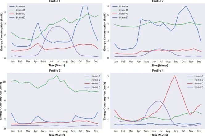
Figure 1 provides year-wide representation of consumption profiles for each household in the Smart Star dataset, as extracted by the Deep COLA algorithm. As evidenced, there are 4 profiles that can be clearly distinguished in Homes A, B, C and D, in terms of low, medium and high en-ergy consumption (Kw/h). However, for each house the most dominant profile varied, since behavioral usage of individual appliances by consumers is different in most cases. In parallel, each profile for a given household results from a combined view over appliances that contributed towards a given energy consumption value over time, which may be correlated with environmental aspects (e.g. humidity). The characteristics of
these load profiles are described using the shape of the profile and the consumption at specific points in time. For instance, the load profiles 1, 2 and 3 of Home B show high energy consumption, except profile 4 with a medium energy consumption. Additionally, it bears less troughs and variations as compared to Home A in load profiles 1 and 2. Based on its load profiles, Home C usually consumes lower energy across the year. However, the profile 4 of Home C indicates that it consumes a lot more energy between July and November, as compared to the other homes. The load profiles shown in Figure 1 can assist utility providers to develop demand response programs for particular homes that consume more energy and have potential to shift demands. Hence, we demonstrate next that the produced profiles have assisted in composing three associations (see Table II): appliance-to-appliance, appliance-to-time and appliance-to-environment.
1) Appliance-to-appliance
Table II demonstrates appliance-to-appliance relationships which are associated with each profile generated from year-wide clustering presented in Figure 1. Each sequence of appliances from left to right depicts the order in which they are most likely to be operated in each home. Profile 1 bears similar characteristics for each home, in which appliances have the same associations. This indicates that this profile is associated with a consumer who often performs daily activities in a similar fashion. For instance, in Home A, the consumer is likely to spend more time throughout the year in the kitchen due to appliance associations (i.e. microwave, dishwasher and fridge). Based on appliance-to-time analysis associated with this profile (see the next sub-section), it was also revealed that when a microwave is being operated, it is highly likely that simultaneously, or within a few minutes, a consumer may use a dishwasher and during this time a fridge is operating at high mode as well. We have also identified that parallel and highly frequent use of the FurnaceHRV appliance, which is used for kitchen ventilation, indicates cooking habits of a consumer. On the other hand, the homes with profiles 3 and 4 have a better internal environment due to less operations of FurnaceHRV; thus there is the minimal use of ventilation while cooking.
Moreover, throughout all the other identified profiles, con-sumer behavior is more varied in comparison to profile 1. Thus, there is less similarity in terms of domestic habits.
2) Appliance-to-time
Figure 1 complements Table II as it demonstrates a high-level view of year-wide maximum consumption distribution over four profiles. Hence, a more general appliance-to-time association may be profiled based on most prevalent profiles in three aforementioned consumption categories. For instance,
Fig. 1: Profiles in the 4 Smart Star homes based on the the lowest, medium and highest energy consumption clusters. TABLE II: Year-wide appliance-to-appliance association (Smart Star Dataset)
Profile No. Household Appliances
1 Home A FurnaceHRV Microwave DishWasher Fridge Dryer BedroomLights
Home B FurnaceHRV Microwave Dishwasher Fridge Dryer BedroomLights
Home C FurnaceHRV Microwave Dishwasher Fridge Dryer BedroomLights
Home D FurnaceHRV Microwave Dishwasher Fridge Dryer BedroomLights
2 Home A Dishwasher Fridge BedroomLights Microwave Dryer FurnaceHRV
Home B BedroomLights Fridge Dishwasher Microwave FurnaceHRV Dryer
Home C Dryer BedroomLights Microwave Fridge Dishwasher FurnaceHRV
Home D BedroomLights Microwave Fridge FurnaceHRV Dryer Dishwasher
3 Home A Dishwasher Fridge Dryer Microwave BedroomLights FurnaceHRV
Home B Dishwasher Dryer Microwave BedroomLights Fridge FurnaceHRV
Home C Dryer Microwave Dishwasher BedroomLights Fridge FurnaceHRV
Home D Dishwasher Microwave Dryer BedroomLights Fridge FurnaceHRV
4 Home A Dishwasher Fridge BedroomLights Microwave Dryer FurnaceHRV
Home B Dishwasher Microwave Dryer BedroomLights Fridge FurnaceHRV
Home C Dryer Dishwasher Microwave BedroomLights Fridge FurnaceHRV
Home D Dishwasher Microwave Dryer BedroomLights Fridge FurnaceHRV
profile 3 is present in Homes A, C and D and is regarded as a low energy profile, with consumption around 1.3kw/h for the whole year. Similarly, Homes A, B and D share similar consumption characteristics of around 1kw/h and are associated with profile 4. Homes that consume energy of3kw/h and beyond belong to a high energy profile. Figure 1 indicates that Home B belongs to all four profiles (low, medium and high). These profiles illustrate variations in energy with respect to time.
3) Appliance-to-environment
The appliance-to-environment association is identified by correlating environmental inputs with actual energy utilisation by individual appliances in each profile. This association quantifies the effect on appliances energy consumption with respect to variations in temperature, humidity, geography and social events. Our clustering algorithm has identified that
profile 1 has higher relevance to the environment factors and can provide an insight in terms of internal household environ-mental conditions. We have identified that FurnaceHRV has more significance for profile 1 in Table II, as compared to profiles 3 and 4. FurnaceHRV directly balances the humidity level, which is inversely proportional to air temperature in the household. Naturally, extremely low or high temperatures will cause an interruption in the humidity level, which will require FurnaceHRV to consume more energy to adjust the humidity level. The findings show that environmental factors affect energy consumption and proper building structure assists in reducing the consumption.
C. Deep COLA Performance Assessment
Table III presents a comparison between Deep COLA and commonly used clustering algorithms, K-means, DBSCAN
TABLE III: Computational time comparison of Deep COLA with K-means, DBSCAN and SOM
Dataset Homes Consumption Period No. of Records Deep COLA (sec) K-means (sec) DBSCAN (sec) SOM (sec)
UK-DALE 1 1 day 12560 164 196 1500 230
UK-DALE 1 1 Week 84168 750 900 2100 1120
Smart Star 4 1 Year 17521 200 260 430 540
and SOM (Sefl-Organizing Maps), in terms of their compu-tational costs. It is evident that, in comparison to the rest, Deep COLA requires less time to compose clusters across all the datasets. The processing time of the Deep COLA algorithm involves time required for dimensional reduction and extracting the profiles. In contrast with our scheme, where clusters are created adaptively, the K-means and DBSCAN al-gorithms require additional processing to interpret and validate clusters’ consistency (e.g. with the use of k-dist, Elbow or Silhouette metrics) in order to specify the number of clusters (k). The metrics k-dist, Elbow and Silhouette measure the distortion in data by using various values for (k). The stopping condition is at a sudden decline of average distortion and it provides the optimal value for (k). The SOM requires to select the number of nodes in the output layer to cluster data. It performs dimensionality reduction to visualise data with large dimensions. Moreover, Deep COLA inherits deep neural network properties, thus it is much more efficient in handling larger datasets than the other two approaches, as evidenced particularly for week-wide profiling in Table III.
Evaluation of the Deep COLA performance
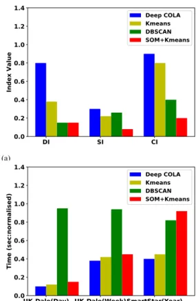
The quality of clusters produced by an algorithm mainly depends on higher inter-cluster and lower intra-cluster sepa-ration. For the performance evaluation of Deep COLA, three validity indexes are selected, DI, SI and CI. These indexes are well suited for measuring the compactness and separation of clusters and particularly depend upon data itself. DI is to identify groups of clusters that maximise inter-cluster and minimise intra-cluster separation. SI allows to compare the cohesion and separation of clusters. CI is based on Analysis of Variance (ANOVA) and is mostly suitable for spherical clusters. ANOVA allows to estimate variations among and be-tween clusters. Figure 2 illustrates the comparison of distance measures and index metrics. Subfigures (a) to (c) depict graphs of DI, SI and CI, using Euclidean distance and Dynamic Time Warping (DTW). Values of the indexes mainly depend on random initial weights, which have been selected at the beginning of training. The drops of index values in the 4th and 5th experiments, in subfigures (a) and (b) represent that initial weights did not provide ability to lower optimisation errors during training and as a result clusters were not formed properly. Figure 3 provides a visual representation of Deep COLA’s comparison against the other algorithms based on clustering accuracy and computational cost. In figure 3(a), higher values of DI, SI and CI indexes represent better clustering, where CI index values have been normalised to show them on the graph.
The DI, SI and CI metrics in Figure 3(a) illustrate that Deep COLA performed better in comparison with the other algorithms. DI, SI and CI are internal evaluation techniques for the clusters, which are based on the dataset itself. The
TABLE IV: Deep COLA evaluation
Exp. No. of Neurons Layers/Clusters Distance DI SI CI 1 [43, 50, 1] 3/7 Euclidean 0.87 0.24 6230 3/7 DTW 0.66 0.27 1451 2 [43, 45, 45, 1] 4/7 Euclidean 0.77 0.20 15146 4/2 DTW 0.83 0.24 4.60 3 [43, 50, 50, 1] 4/11 Euclidean 0.95 0.19 4317 4/20 DTW 0.89 0.18 17072 4 [43, 55, 45, 1] 4/9 Euclidean 0.89 0.24 16873 4/12 DTW 0.34 0.18 1633 5 [43, 55, 50, 1] 4/12 Euclidean 0.93 0.18 8504 4/2 DTW 0.73 0.05 3.2 6 [43, 55, 55, 1] 4/20 Euclidean 0.93 0.19 20856 4/10 DTW 0.99 0.21 4837
internal evaluation is carried out using two characteristics of the clusters, i.e. the compactness and well separation of the clusters. Deep COLA identifies these two characteristics using the capabilities of deep representational learning, in which data representations are extracted on a layer-by-layer basis. The compactness and separation characteristics are essential for the efficient profiling of energy consumption of individual appliances. The K-means algorithm performs clustering on the original dataset, which contains a large number of features (i.e. 53 appliances). Due to the high dimensionality of the data, K-means requires a high computational cost in order to extract load profiles. Additionally, in this high dimension, all the data points become similar to each other. However, Deep COLA is based on the concept of first reducing the dimensionality of the data and then applying competitive learning to find clusters. Thus, the dimensionality reduction and clustering loss (member assignment to clusters) are performed simul-taneously, so better clusters are found in lower dimensional datasets. Table IV shows the results of the experiments for various parameter configurations and index metric values only for Deep COLA. It highlights the effect that a different number of layers and neurons in each layer have on the accuracy of the clusters. In deep neural networks, the transformation of the input varies based on the number of layers and their neurons. Therefore, different clusters are produced by varying the network configuration. Initially, the experiments were conducted using 3 layers to calculate DI, SI and CI values. The three indexes show a decreasing trend for extremely large networks. The maximum DI, SI and CI values are required to obtain compact clusters. However, in large networks, due to overfitting, the indexes show lower values.
Further Comparison of Deep COLA with other algorithms We now compare Deep COLA against the K-means, DB-SCAN and SOM algorithms, in terms of the clustering per-formance. SOM is used as a hybrid algorithm with K-means for the purpose of dimensionality reduction. The process of clustering energy consumption using these algorithms involves first applying SOM to an original dataset, which consists of all
1 2 3 4 5 6 7 8 9 10 Experiment No. 0.0 0.2 0.4 0.6 0.8 1.0 1.2 Ind ex Va lue Dunn Index Euclidean DTW (a) 1 2 3 4 5 6 7 8 9 10 Experiment No. 0.00 0.05 0.10 0.15 0.20 0.25 0.30 Ind ex Va lue Silhuette Score Index Euclidean DTW (b) 1 2 3 4 5 6 7 8 9 10 Experiment No. 0 5000 10000 15000 20000 Ind ex Va lue Calinskiharabasz Index Euclidean DTW (c)
Fig. 2: Distance measures and index metric comparison
DI SI CI 0.0 0.2 0.4 0.6 0.8 1.0 1.2 1.4 Ind ex Va lue Deep COLA Kmeans DBSCAN SOM+Kmeans (a) UK-Dale(Day) UK-Dale(Week)SmartStar(Year) 0.0 0.2 0.4 0.6 0.8 1.0 1.2 1.4 Time (s ec :nor ma lis ed ) Deep COLA Kmeans DBSCAN SOM+Kmeans (b)
Fig. 3: (a) Clustering accuracy and (b) computational time comparison of Deep COLA with K-means, DBSCAN and SOM
feature vectors, in order to obtain a low dimensional feature vector. The purpose of applying SOM for dimensionality reduction is that, in case of higher dimensions, the K-means performance starts degrading due to the use of Euclidean distance. As a result, distance converges between two data points, in extremely high dimensions, so the minimum and maximum distances become equal. Therefore, clustering is usually performed on a low dimensional feature vector using algorithms such as K-means. This is why K-means is used with SOM to cluster household energy consumption. SOM requires more parameters to specify the dimensionality of the final reduced feature vector. K-means also requires the number of clusters to be specified in advance. Figure 3 (b) illustrates a comparison between Deep COLA and other algorithms using Euclidean distance. For Deep COLA, both distance measures (Euclidean distance and DTW) are used, while other
algorithms are assessed using Euclidean distance only. The load profiles do not show a linear trend over time and depend upon various factors in the household, such as a user’s daily activity, environment and economic factors. The distance measures, i.e. Euclidean and DTW, compute the similarity between load profiles in different ways. For instance, the Euclidean distance metric is based on the assumption that the data points in the load profiles are linearly identical and bear an exact match. On the other hand, the DTW distance metric does not assume a linear match between the load profiles and learns the underlying patterns for calculating the similarity. To group similar appliances on a day-to-day basis, the DTW distance measure provides an efficient way to calculate cor-relation among daily activities. For example, the time of use of appliances, e.g. toaster, oven, TV, laptop, etc., may vary daily in the household, based on the user’s preference. As a result, this will have an effect on energy consumption, in terms of shifting and translating load profiles. The DTW distance measure reduces the effect of shifting and translation of energy consumption in time. DTW performs elastic transformations to classify load profiles with similar characteristics. Therefore, DTW is more suitable to capture variations in consumption of appliances as compared to Euclidean distance.
VI. APPLICABILITY OFLOADPROFILING INSMARTGRID
Many decision making processes in the smart grid domain depend on profiling energy consumption and understanding human behaviour in domestic and commercial sectors. These decisions are made to plan energy generation, buy or sell energy during peak and off-peak hours and develop various demand response programs to reduce or shift energy con-sumption during peak hours. The reduction or shifting of peak hour energy consumption provides benefits related to a reduction in carbon emissions, less chance of system failure due to heavy load, and most importantly the cost to maintain a reliable power supply. The profiling of energy consumption, obtained through the proposed algorithm, assists in developing successful demand response programs. This is because it analyses flat, medium and high demand energy consumption appliances.
VII. CONCLUSION
The efficient profiling of appliance-level energy consump-tion, in residential households, is a fundamental building block in future HEMSs. In this paper, we have argued that profil-ing should be done in the context of appliance-to-appliance,
appliance-to-time and appliance-to-environment associations. We have thus proposed Deep COLA, a novel Deep Compet-itive Learning-based Algorithm, to profile appliance-level en-ergy consumption. Through our evaluation, over real datasets, we have demonstrated the superiority of our scheme over com-monly used methods. This is achieved by avoiding the a-priori selection of the cluster number in the scheme, whilst being capable of composing accurate and computationally optimal day, week and year-wide appliance-level consumption profiles. Given the clustering enabled by Deep COLA, we have also demonstrated the feasibility of identifying end-user habitual insights over the three aforementioned associations to aid in developing various demand response programs. We envision that Deep COLA can become a core element within future HEMSs. Furthermore, we aim to implement Deep COLA together with Spark and Hadoop, which will provide parallel computation capabilities to assist Deep COLA in reducing computational time for large energy consumption datasets and thus increase clustering efficiency.
REFERENCES
[1] S. Z. et al, “Appliance flexibility analysis considering user’s behavior in home energy management system using smart plugs,”IEEE Transactions on Industrial Electronics, vol. 66, no. 2, pp. 1–1, 2018.
[2] C. Magazzino, “Is per capita energy use stationary? time series evidence for the emu countries,” Energy Exploration & Exploitation, vol. 35, no. 1, p. 1, 2017.
[3] J. M. et al, “Residential load scheduling in smart grid: a cost efficiency perspective,”IEEE Transactions on Smart Grid, vol. 7, no. 2, 2016. [4] S. et al, “Using consumer behavior data to reduce energy consumption
in smart homes: Applying machine learning to save energy without lowering comfort of inhabitants,”ICMLA 2015, p. 1123, 2016. [5] S. Rollins and N. Banerjee, “Using rule mining to understand appliance
energy consumption patterns,”PerCom 2014, pp. 29–37, 2014. [6] A. Albert and R. Rajagopal, “Smart Meter Driven Segmentation : What
Your Consumption Says About You,” IEEE Transactions on Power Systems, vol. 28, no. 4, pp. 4019–4030, 2013.
[7] A. K. M. et al, “Power consumption profiling using energy time-frequency distributions in smart grids,”IEEE Communications Letters, vol. 19, no. 1, pp. 46–49, 2015.
[8] R. Lin, B. Wu, and Y. Su, “An Adaptive Weighted Pearson Similarity Measurement Method for Load Curve Clustering,”Energies, vol. 11, no. 9, p. 2466, 2018.
[9] S. Ryu, H. Choi, H. Lee, H. Kim, and V. W. S. Wong, “Residential Load Profile Clustering via Deep Convolutional Autoencoder,”IEEE International Conference on Communications, Control, and Computing Technologies for Smart Grids (SmartGridComm), 2018.
[10] J. S. Chou and N. S. Truong, “Cloud forecasting system for monitoring and alerting of energy use by home appliances,” Applied Energy, vol. 249, pp. 166–177, 2019.
[11] R. Ford, J. Stephenson, N. Brown, and W. Stiehler,Energy transitions : home energy management systems (HEMS). Centre for Sustainability, University of Otago, New Zealand, 2014.
[12] A. Satre-Meloy, M. Diakonova, and P. Gr¨unewald, “Cluster analysis and prediction of residential peak demand profiles using occupant activity data,”Applied Energy, vol. 260, 2020.
[13] F. Issi and O. Kaplan, “The determination of load profiles and power consumptions of home appliances,”Energies, vol. 11, no. 3, 2018. [14] J. Lai, H. Zhou, W. Hu, D. Zhou, and L. Zhong, “Smart Demand
Re-sponse Based on Smart Homes,”Mathematical Problems in Engineering, vol. 2015, 2015.
[15] J. Kelly and W. Knottenbelt, “The UK-DALE dataset, domestic appliance-level electricity demand and whole-house demand from five UK homes,”Scientific Data, vol. 2, p. 150007, 2015.
[16] X. Glorot and Y. Bengio, “Understanding the difficulty of training deep feedforward neural networks,”13th International Conference on Artificial Intelligence and Statistics, vol. 9, pp. 249–256, 2010.
Ghulam Mohi-Ud-Din received M.Sc. degree in Computer Science from Bradford University, (UK) and PhD degree in Computer Science from Liver-pool John Moores University, (UK). His research interests include artificial intelligence, deep learning approaches, big data, cyber security, telecommunica-tion, and application specific architectures for IoT-based electronics systems.
Angelos K. Marneridesis an Associate Professor of Secure Networked Systems in the School of Computing Science at University of Glasgow (UoG), UK. Dr. Marnerides leads a group Glasgow Systems Section (GLASS) dealing with applied security and resilience research for Internet-enabled cyber physi-cal systems. Prior to that he was an Assistant Profes-sor at the School of Computing and Communications at Lancaster University and the founding director of innovative Digital Infrastructure Defense (i-DID) group. His research has received significant funding from industry (e.g., Fujitsu, BAE, Raytheon), governmental bodies (e.g., EU, IUK, EPSRC) and he has been invited to serve as an expert reviewer in grant proposal panels (e.g., Chilean research commission). He has been member of IEEE and ACM since 2007 and served as a Technical Program Committee (TPC) member, TPC track and workshop co-chair and organiser for several IEEE and IFIP conferences including IEEE ICC, IEEE GLOBECOM, IEEE INFOCOM, IEEE CCNC, IFIP Networking, IEEE WoWMoM, and IEEE GLOBALSIP leading him to receive IEEE ComSoc contribution awards in 2016 and 2018. He holds an MSc (’07) and PhD (’11) in Computer Science from Lancaster University and held postdoctoral and visiting researcher positions at Carnegie Mellon University (USA), University of Porto (Portugal), Lancaster University (UK) and University College London (UK).
Qi Shi is a Professor in Computer Security and Director of PROTECT Research Centre in Depart-ment of Computer Science at Liverpool John Moores University (LJMU) in UK. He received his PhD in Computing from Dalian University of Technology, P.R. China. He then worked as a Research Associate at University of York in UK. Qi then joined LJMU, working as a Lecturer and then a Reader before becoming a Professor. He has many years research experience in a number of areas, e.g. IoT security, secure service composition, privacy-preserving data aggregation, cryptography, computer forensics, formal security models and cloud security. He has published over 250 papers in international conference proceedings and journals, and served in a number of conference IPCs and journal editorial boards. He has also played a key role in many funded research and development projects related to his research topics.
Chelsea Dobbinsreceived BSc (Hons) in Software Engineering and PhD in Computer Science from Liverpool John Moores University (LJMU), in 2010 and 2014, respectively. Currently, she is a Senior Lecturer within the School of Information Tech-nology and Electrical Engineering (ITEE) at The University of Queensland in Brisbane, Australia. She has been the recipient of a research grant from the UK’s Engineering and Physical Sciences Research Council (EPSRC) and has also received an ACM Computing Review Notable Article of 2016 award for work related to mining multivariate temporal smart mobile data. She is also currently an academic editor for PLOSONE and co-leader of the Empathic Extended Reality Pervasive Computing (EXR-PC) Lab within ITEE.
´
Aine MacDermottis a Senior Lecturer in Cyber Se-curity and IoT in the Department of Computer Sci-ence at Liverpool John Moores University (LJMU) in the UK. She received her PhD in Network Secu-rity from Liverpool John Moores University in 2017, and a first class BSc (Hons) in Computer Forensics in 2011. Previously ´Aine worked as an Associate Tutor in Computing at Edge Hill University for two academic years. Academic research interests include the Internet of Things, critical infrastructure protection, computer network security, collaborative intrusion detection in interconnected networks, and digital forensics – over 25 academic papers have been published to date, presenting and exhibiting both nationally and internationally.