DIPARTIMENTO DI INGEGNERIA DELL'INFORMAZIONE
Non-Parametric Bayesian Methods For
Linear System Identification
Ph.D. candidate Giulia Prando
Advisor Prof. Alessandro Chiuso
Co-Advisor Prof. Gianluigi Pillonetto
Director & Coordinator Prof. Matteo Bertocco
Ph.D. School in Information Engineering . Department of Information Engineering University of Padova 2016
Abstract
Recent contributions have tackled the linear system identification problem by means of non-parametric Bayesian methods, which are built on largely adopted machine learning techniques, such as Gaussian Process regression and kernel-based regularized regression. Following the Bayesian paradigm, these procedures treat the impulse response of the system to be estimated as the realization of a Gaussian process. Typically, a Gaussian prior accounting for stability and smoothness of the impulse response is postulated, as a function of some parameters (called hyper-parameters in the Bayesian framework). These are generally estimated by maximizing the so-called marginal likelihood, i.e. the likelihood after the impulse response has been marginalized out. Once the hyper-parameters have been fixed in this way, the final estimator is computed as the conditional expected value of the impulse response w.r.t. the posterior distribution, which coincides with the minimum variance estimator. Assuming that the identification data are corrupted by Gaussian noise, the above-mentioned estimator coincides with the solution of a regularized estima-tion problem, in which the regularizaestima-tion term is the`2 norm of the impulse response, weighted by the inverse of the prior covariance function (a.k.a. kernel in the machine learning literature).
Recent works have shown how such Bayesian approaches are able to jointly perform esti-mation and model selection, thus overcoming one of the main issues affecting parametric identification procedures, that is complexity selection.
While keeping the classical system identification methods (e.g. Prediction Error Methods and subspace algorithms) as a benchmark for numerical comparison, this thesis extends and analyzes some key aspects of the above-mentioned Bayesian procedure. In particular, four main topics are considered.
Prior design. Adopting Maximum Entropy arguments, a new type of`2 regular-ization is derived: the aim is to penalize the rank of the block Hankel matrix built with Markov coefficients, thus controlling the complexity of the identified model, measured by its McMillan degree. By accounting for the coupling between different input-output
channels, this new prior results particularly suited when dealing for the identification of MIMO systems.
To speed up the computational requirements of the estimation algorithm, a tailored version of the Scaled Gradient Projection algorithm is designed to optimize the marginal likelihood.
Characterization of uncertainty. The confidence sets returned by the non-parametric Bayesian identification algorithm are analyzed and compared with those returned by parametric Prediction Error Methods. The comparison is carried out in the impulse response space, by deriving “particle” versions (i.e. Monte-Carlo approximations) of the standard confidence sets.
Online estimation. The application of the non-parametric Bayesian system identi-fication techniques is extended to an on-line setting, in which new data become available as time goes. Specifically, two key modifications of the original “batch” procedure are proposed in order to meet the real-time requirements. In addition, the identification of time-varying systems is tackled by introducing a forgetting factor in the estimation criterion and by treating it as a hyper-parameter.
Post processing: model reduction. Non-parametric Bayesian identification pro-cedures estimate the unknown system in terms of its impulse response coefficients, thus returning a model with high (possibly infinite) McMillan degree. A tailored procedure is proposed to reduce such model to a lower degree one, which appears more suitable for filtering and control applications. Different criteria for the selection of the order of the reduced model are evaluated and compared.
Acknowledgements
During the last three years I have met special people who have helped me in reaching the results presented in this thesis. Many of them deserve my thanks.
My greatest thanks go to my advisor, Prof. Alessandro Chiuso: thank you for the things you taught me and for the passion you put in guiding me during these three years. I would like to thank Prof. Gianluigi Pillonetto for sharing his inspiring ideas.
My sincere thanks go to my colleague Diego Romeres: working together has been productive and also very funny! I will not forget our long and interesting discussions, which also gladdened our office mates (now they all know what Empirical Bayes and MCMC are. . . )
I also would like to thank Prof. Michael I. Jordan for hosting me in his group at UC Berkeley.
Prof. Lennart Ljung and Prof. Simone Formentin, the reviewers of the first version of this thesis, also deserve my acknowledgement for their insightful comments.
Special thanks go to my office mates, who made these three years unforgettable and have become very good friends in my life. Thanks to Nicoletta and Giulia, who proofread the first draft of this thesis.
Last but not the least, I would like to thank my family: my grandmother, for having supported me in her own way and for having waited for me every evening; my parents for having continuously tried to transmit their faith in my potentialities, even if they still have to understand what I am doing...
Contents
1 Introduction 1
1.1 Outline . . . 4
2 System Identification Methods 9 2.1 System Identification Problem. . . 10
2.2 Prediction Error Methods . . . 13
2.2.1 Transfer Function Models . . . 15
2.2.2 User’s Choices . . . 16
2.2.3 Connection with Maximum Likelihood Estimation . . . 18
2.2.4 Algorithmic Details . . . 19
2.3 Subspace Methods . . . 21
2.3.1 State-Space Models . . . 22
2.3.2 Subspace Methods in Practice. . . 24
2.3.3 User’s choices . . . 35
2.3.4 Algorithmic Details . . . 37
2.4 Non-Parametric Bayesian Methods . . . 37
2.4.1 Non-Parametric Bayesian Methods for SISO systems . . . 39
2.4.2 Non-Parametric Bayesian Methods for MIMO systems . . . 47
2.4.3 Hyperparameters Tuning . . . 52
2.4.4 User’s Choices . . . 56
2.4.5 Algorithmic Details . . . 58
2.5 Model Selection and Validation . . . 65
2.5.1 A Priori Model Class Selection . . . 67
2.5.2 Model Class Selection during the Estimation Stage . . . 67
2.5.3 Model Validation . . . 70
2.6 Bibliographical Notes. . . 72
2.6.1 System Identification Problem . . . 72
2.6.3 Subspace Methods . . . 73
2.6.4 Non-Parametric Bayesian Methods . . . 74
3 Prior Design 77 3.1 Regularization in Prediction Error Methods . . . 80
3.1.1 `2 Regularization . . . 80
3.1.2 `1 Regularization . . . 81
3.2 Regularization in Subspace Methods . . . 83
3.2.1 `2 Regularization . . . 83
3.2.2 `1 Regularization . . . 83
3.3 Regularization in Non-Parametric Bayesian Methods . . . 87
3.3.1 `2 Regularization . . . 87
3.3.2 `1 Regularization . . . 90
3.4 Combining`2 and`1 regularization in Non-parametric Bayesian system identification: a Maximum-Entropy derivation . . . 94
3.4.1 Maximum-Entropy design of stable Hankel-type penalties . . . 95
3.4.2 Identification Algorithm . . . 102
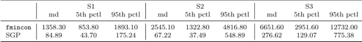
3.4.3 SGP for Marginal Likelihood Optimization . . . 107
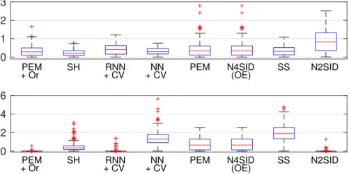
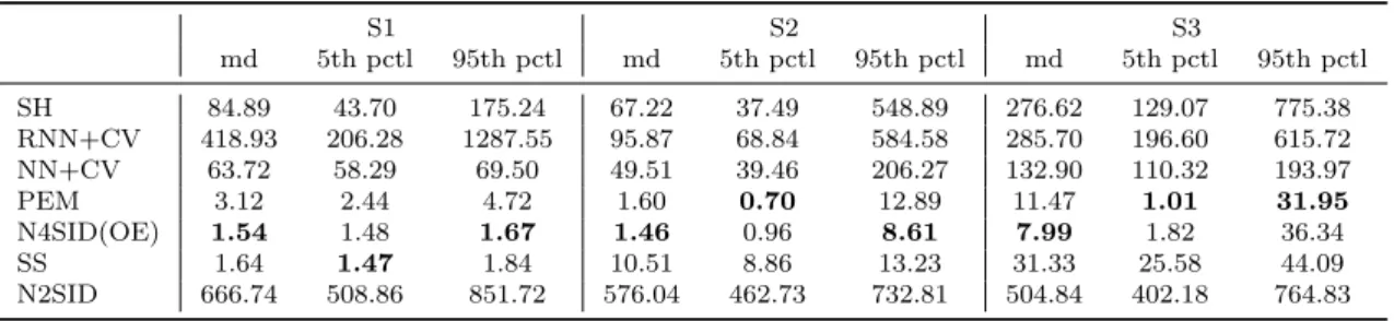
3.5 Numerical Results . . . 108
3.5.1 Data . . . 109
3.5.2 Identification Algorithms . . . 110
3.5.3 Impulse Response Estimate . . . 112
3.5.4 Predictive Performance . . . 112
3.5.5 Estimated Hankel Singular Values . . . 116
3.5.6 Computational Time . . . 119
4 Estimators’ Statistical Properties and Uncertainty 121 4.1 Statistical Properties of Prediction Error Estimates. . . 122
4.1.1 Asymptotic Properties of PEM Estimates . . . 123
4.1.2 Finite-Sample Properties of PEM Estimates . . . 130
4.2 Statistical Properties of Subspace Estimates . . . 132
4.2.1 Consistency . . . 133
4.2.2 Misspecification. . . 133
4.2.3 Asymptotic Distribution of the Parameters Estimate . . . 134
4.2.4 Statistical Efficiency . . . 135
4.3 Statistical Properties of Non-Parametric Bayesian Estimates. . . 135
Contents ix
4.3.2 Misspecification. . . 137
4.3.3 Confidence Intervals . . . 138
4.4 PEM and Non-Parametric Bayesian Methods: a Comparison of the Esti-mators’ Uncertainty . . . 140 4.4.1 PEM . . . 141 4.4.2 Empirical Bayes . . . 143 4.4.3 Full Bayes . . . 143 4.5 Numerical Results . . . 143 4.5.1 Data . . . 143 4.5.2 Identification Algorithms . . . 144
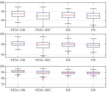
4.5.3 Impulse Response Estimates . . . 144
4.5.4 Returned Confidence Sets . . . 147
5 On-line System Identification 155 5.1 On-Line Identification with Prediction Error Methods . . . 156
5.1.1 Dealing with Time-Varying Systems . . . 159
5.2 On-Line Identification with Subspace Methods . . . 162
5.3 On-Line Identification with Non-Parametric Bayesian Methods . . . 163
5.3.1 Dealing with Time-Varying Systems . . . 166
5.4 Numerical Results . . . 170
5.4.1 Time-Invariant Systems . . . 170
5.4.2 Time-Varying Systems . . . 175
6 Model Reduction 179 6.1 Model Reduction in Control System Theory . . . 181
6.1.1 SVD-based Methods . . . 182
6.1.2 Krylov-based Methods . . . 185
6.1.3 SVD and Krylov-based methods . . . 186
6.2 Model Reduction in System Identification . . . 187
6.2.1 Model Reduction and Prediction Error Methods . . . 188
6.2.2 Model Reduction and Subspace Methods . . . 191
6.2.3 Model Reduction and Non-parametric Bayesian Methods . . . 191
6.3 From Non-parametric to Parametric Models: Model Reduction Meets Order Selection . . . 193
6.3.1 Choice of the Reduced Order . . . 196
6.4 Numerical Results . . . 198
6.4.2 Identification Algorithms . . . 200 6.4.3 Impulse Response Estimates and Selected Low-Orders . . . 202
7 Conclusions and Future Work 217
A Reproducing Kernel Hilbert Spaces 223
B Connections between EM and other algorithms 227
B.1 Connection between EM and Gradient Methods. . . 228 B.2 Connection between EM and Iterative Reweighted Methods . . . 229
Operators
:= The left side is defined by the right side =: The right side is defined by the left side
kxk2 Euclidean norm of vector x
kxk2
Q x>Qx withQ symmetric positive definite weighting matrix
kAkF Frobenius norm of matrixA
⊗ Kronecker product
0d Zero-vector of sized
{x(t)} {x(t);t∈Z}
arg min f(x) Value ofx which minimizesf(x)
blockdiag(A, B) Block diagonal matrix built with matrices Aand B
Cov(x) Covariance matrix of the random vector x
∂
∂θ f(θ, x) Partial derivative off with respect toθ det(A) Determinant of matrix A
E[x] Expectation of the random variable (or vector) x
δt,s Kronecker delta
Dfˆy(x) Matricial degrees of freedom of estimator ˆy expressed as
func-tion of x
diag(v) s Diagonal matrix having the vectorv on the diagonal dist
−→ Convergence in distribution dim θ Dimension of the column vectorθ
f0(x) Gradient off(x); a row vector of dimension dimxiff is scalar
valued
f00(x) Hessian of f(x)
G Square Hankel matrix built with the coefficients of the sequence
{g(k)}Nk=1 ¯
G Shifted square Hankel matrix built with the coefficients of the sequence {g(k)}Nk=1
H(·) Entropy function
Id Identity matrix of size d×d
A−1 Inverse of matrix A
A† Moore-Penrose pseudo-inverse of A
N(µ,Σ) Gaussian distribution with mean µand covariance Σ
q Shift operator
Contents xiii
N+ N\ {0}
Pr{A} Probability of event A px(·) PDF of random vector x
R Set of real numbers
R+ Set of positive real numbers: R+ := [0,∞) Rd Euclidean d-dimensional space
Rm×n Space of real matrices with m rows andn columns
range(A) Column space of matrixA
rank(A) Rank of matrixA
Tr[A] Trace of matrix A A> Transpose of matrixA
Var(x) Variance of the random vectorx
vec(A) Vectorization (column-wise) of matrixA
x∼p(x) The random variable x is distributed according to the
proba-bility distributionp(x)
xi.i.d∼ p(x) x is identically independently distributed according to
distri-bution p(x)
yst {y(s), y(s+ 1), ..., y(t)}
yt {y(1), y(2), ..., y(t)}
Symbols
DM Set of values over whichθ ranges for the model structureM e(t) Disturbance variable at timet; typically {e(t)}∞t=0 is assumed
to be white noise
ε(t, θ) Prediction errory(t)−yˆ(t|θ)
G(q) Transfer function fromu toy
G(q;θ) Transfer function fromu toy in a model M(θ) g(k) k-th sample of the impulse response from u toy
G = (A, B, C, D) Compact notation for a state-space system described by the
matrices A, B, C and D H(q) Transfer function frome toy
H(q;θ) Transfer function frome toy in a modelM(θ)
h(k) k-th sample of the impulse response from etoy
M Model structure (i.e. a mapping from the parameter space to a set of models)
M(θ) Model corresponding to the parameter valueθ
M Set of models
p(x) Probability distribution of the random variablex px(·) Probability density function of the random variable x ϕ(t) Regressors vector at timet
ψ(t, θ) Gradient of ˆy(t|θ) w.r.tθ
S The true data generating system
Sx(ω) Spectrum of the signal{x(t)}
Σ Innovation variance for multi-variable systems, defined as Σ = diag([σ1,· · ·, σp])
e
Σ Σ⊗IN
σ Innovation variance for SISO systems
θ Parameter vector
ˆ
θ Estimate ofθ computed using the datasetZN u(t) Input variable at time t
v(t) Disturbance variable at timet
VN(θ,DN) Parametric loss function defined on the datasetDN
y(t) Output variable at time t
ˆ
y(t) Predicted output at timet based on the data{y(t−1), u(t−
1), ..., y(1), u(1)}
ˆ
y(t|θ) Predicted output at time tusing a modelM(θ) and based on the data{y(t−1), u(t−1), ..., y(1), u(1)}
DN Dataset composed ofN input-output data pairs, namelyDN =
Contents xv
Acronyms
ARMA AutoRegressive Moving Average
ARMAX AutoRegressive Moving Average with eXternal input
BIBO Bounded Input Bounded Output
EM Expectation Maximization
FIR Finite Impulse Response
GLS Generalized Least Squares
GP Gaussian Process
GPR Gaussian Process Regression
i.i.d. identically independently distributed
LTI Linear Time-Invariant
LS Least Squares
MAP Maximum A Posteriori
MCMC Markov Chain Monte Carlo
MIMO Multi Input Multi Output
MLE Maximum Likelihood Estimate
MSE Mean Square Error
OE Output Error
PE Prediction Error
PEM Prediction Error Methods
ReLS Regularized Least Squares
RKHS Reproducing Kernel Hilbert Space
RLS Recursive Least Squares
RPEM Recursive Prediction Error Methods SISO Single Input Single Output
SGP Scaled Gradient Projection
s.t. subject to
SVD Singular Value Decomposition
w.p. With probability
1
Control systems engineering aims at forcing a dynamical system to have a desired behaviour. The success of the discipline is highly dependent on the availability of an accurate mathematical model of the system to be controlled. In the continuous-time domain, such model consists of differential equations, while in the discrete-time regime it is described by a set of difference equations. A model may not only be used for the design of a desired controller, but also for simulation purposes, fault detection, quality control, etc. In addition, the presence of a model becomes essential when experiments performed through the real system are too expensive or too dangerous.
Physics first principles may provide a tool to derive such models; however, while in most cases the dynamical behaviour of interest could be too complex to be described through physical laws, in other cases, the physical model could not be suitable for its intended use. Indeed, the quality of a model should always be assessed in terms of its purpose: while a model may be good for simulation, it may not be the best one for control. Model complexity also plays a crucial role in control system engineering, where accuracy should always be traded-off with complexity: a complex model will lead to a complex controller and in turn to implementation and robustness issues. These considerations explain the development of techniques allowing to infer the mathematical model of a dynamical system from experimental data. System Identification is the discipline collecting all these
procedures. As such, system identification appears as a preliminary step of any control system application, ranging from industrial plants to aeronautical vehicles, from home automation to humanoid robots.
The standard set-up of a system identification problem involves a set of input data, which are fed into the system under consideration, and a set of corresponding output data, recording the response of the system to the chosen input signal. The measurements, provided by suitable sensors, are typically affected by disturbances, whose presence has to be accounted for in the subsequent estimation stage. Most research in system identification has considered only noisy output data, while less attention has been devoted to the presence of disturbances on both input and output measurements (errors-in-variables models).
The described set-up can be fixed by the user (experiment design) according to the intended application. For instance, the user may choose the signals to measure and the excitation signal (input design) in order to maximize the information acquired from the performed experiment. Once the data are recorded, a pre-processing stage may be performed in order to remove undesired artefacts (e.g high-frequency disturbances, missing data, outliers, etc.).
3
during which the data drive the search of the best model within the chosen model class. At this stage, a crucial role is played by the selection of the model class: it may be dictated by some a priori knowledge or, more frequently, by specific statistical procedures or by the chosen inference approach. This step is of primary concern not only in the context of system identification, but also in many statistical and learning applications, giving rise to a wide literature on this topic. Due to its importance, the theme of model selection will be widely discussed in the remainder of the manuscript.
The quality of the model returned by the inference procedure is then assessed (model validation). If the model does not properly describe the observed data or if it does not
appear suitable for its intended use, the identification procedure has to be reviewed and a new model should be estimated.
The distinguishing tract of the estimation performed in system identification is the tem-poral relation present in the data: since the future output of a dynamical system depends on past input values, the prediction performed by the estimated model will be based on past measured input and outputs. System identification shares this characteristics with
econometrics, the discipline which analyses economic data, trying to extract information from them. With the first works dated back at the end of the 19th century, econometrics has a longer tradition than system identification, which instead arose at the end of the 1950s, when the term was coined by Zadeh. However, the roots of system identification lie on the theory of stationary stochastic processes, which was mainly developed by the econometrics and times series communities between 1920 and 1970.
Two seminal papers, both published in 1965, paved the way for the future development of the two most common system identification techniques. The first work, due to Ho and Kalman, gave birth to the deterministic realization theory, thus laying the foundation of the subspace identification algorithms which blossomed in the Nineties. Åström and Bohlin, authors of the second seminal paper, introduced into the control community concepts and terminology coming from the econometrics field, specifically the Maximum Likelihood estimation of the coefficients of difference equation models (known as ARMA, ARMAX, etc.). The whole family of Prediction Error identification methods originated from this work and dominated the system identification field until the Nineties, when the lack of robust tools for the estimation of MIMO systems brought new interest on the realization approach. This renewed appeal led to the the development of subspace algorithms, which became the main focus of system identification research in the 1990s and in the early 2000s.
In parallel with these two main approaches, the Nineties awoke the interest for frequency domain identification with the aim of meeting the progresses reached by robust control
community, whose tools applied in the frequency domain. Another important research line arising in that period regarded the goal-oriented identification: the experiment design and the estimation stages were optimally designed in order to directly take into account the intended use of the model; thus, identification for control and optimal experiment design for control became hot topics around 1990.
The 1990s and the 2000s were also characterized by the wide development of the statistical learning and machine learning fields, with the introduction of new types of regularization, of the Support Vector Machines and with the application of neural networks. Even if many tools adopted by these communities could have been relevant for the system identification problem, only around 2010 some of them were extended to the control community for the estimation of dynamical systems. In particular, non-parametric Bayesian approaches relying on Gaussian Process Regression and on RKHS (Reproducing Kernel Hilbert Space) theory were introduced with the main goal of solving one of the crucial limitations affecting the older system identification techniques, that is the search for the best model structure. Indeed, while subspace methods overcame the issue of model parametrization through the estimation of a state-space model, model order (equivalently, complexity) selection still remained an open problem. Differently from the well-established system identification procedures, which require an a-priori choice of model complexity, Gaussian Process Regression provides an implicit way of dealing with the well-known bias-variance trade-off, allowing to jointly perform estimation and complexity selection.
This manuscript intends to offer new insights on the recently developed non-parametric Bayesian technique for system identification: analysis of some key properties as well as extensions of the original procedure will be provided. In an attempt to give continuity to the research in system identification, the investigation will consider the older approaches (specifically, Prediction Error Methods and subspace algorithms) as a benchmark for
comparison.
In-line with the approach taken in the machine learning community, the innovative results will be mainly presented in an experimental way, meaning that the effectiveness of the proposed techniques will be mainly numerically validated.
1.1
Outline
The thesis aims at providing an overview of the three main system identification techniques, which have so far populated the literature of the field (that is, Prediction Error Methods, subspace algorithms and the recently developed non-parametric Bayesian approach). Special attention will be given to the latter with the purpose of understanding its pros
1.1 Outline 5
and cons, as well as of extending it in order to satisfy specific estimation requirements (such as real-time constraints or model complexity constraints). In addition, several links with the other two main families of identification algorithms will be highlighted.
A brief outline of the manuscript is provided in the following.
Chapter 2 is dedicated to the formal presentation of the linear system identification problem and to the illustration of the three main approaches to deal with it, i.e. the above-mentioned Prediction Error Methods, subspace techniques and non-parametric Bayesian approaches. The description is enriched by details on the algorithmic implementation and on the choices that have to be taken by the user. The chapter concludes with a brief overview of classical model validation techniques.
Chapter 3 focuses on the role of regularization in system identification. After a brief introduction on the use of regularization in statistics and learning applications, an overview of the system identification approaches relying on`2- and`1-type regularization is provided. While `2-type penalties are adopted in order to enforce both numerical robustness and BIBO stability of the estimated system,`1-type regularization is mainly
exploited for structure detection.
Recalling that the regularizer choice translates into the prior design when a Bayesian (probabilistic) framework is adopted, a maximum entropy argument is exploited to derive a new type of prior distribution to be used in the non-parametric Bayesian approach. Following the idea of elastic net in statistical learning, the proposed prior leads to a combination of`1and`2regularization, thus enforcing stability and structure constraints. This chapter is based on the results presented on the papers:
Prando G., Pillonetto G., and Chiuso A. The role of rank penalties in linear system identification. InProc. of 17th IFAC Symposium on System Identification, SYSID, Beijing, 2015
Prando G., Chiuso A., and Pillonetto G.Bayesian and regularization approaches to multivariable linear system identification: the role of rank penalties. InProc. of IEEE CDC, 2014
Prando G., Chiuso A., and Pillonetto G. Maximum entropy vector kernels for mimo system identification. arXiv preprint arXiv:1508.02865, Automatica (accepted as regular paper), 2017
Chapter 4 is devoted to the analysis of the statistical properties of the estimate returned by a system identification procedure. Here the main focus will be on Prediction Error Methods and non-parametric Bayesian techniques: a comparison of the uncertainty (measured in terms of confidence sets) characterizing the obtained estimators will be drawn. The intrinsic difference between the two approaches (namely, the parametric/non-parametric nature) makes the comparison a bit tricky. To overcome the issue, a sampling approach is adopted, leading to the definition of “particle” confidence sets. The reported comparison is based on the results presented on the paper:
Prando G., Romeres D., Pillonetto G., and Chiuso A. Classical vs. bayesian methods for linear system identification: point estimators and confidence sets. InProc. of ECC, 2016a
Chapter 5 deals with the problem of real-time identification, which would allow to update the system estimate as soon as new data arrive, as well as to track possible changes of the system parameters. This problem has been largely considered in the system identification literature, leading to the development of recursive algorithms both for Prediction Error Methods and for subspace algorithms. The first part of the chapter briefly reviews the real-time methods which have been proposed in the literature. The second part introduces a real-time reformulation of the “off-line” algorithm used to compute the non-parametric Bayesian estimator. By means of efficient updates of the data-related entities and of numerical expedients, a fast and robust algorithm is developed. The on-line reformulation of non-parametric Bayesian methods is based on the papers:
Romeres D., Prando G., Pillonetto G., and Chiuso A. On-line bayesian system identification. In Proc. of ECC, 2016
Prando G., Romeres D., and Chiuso A. Online identification of time-varying systems: a bayesian approach. InProc. of IEEE CDC, 2016b
Chapter 6 considers the possibility of combining parametric and non-parametric approaches in order to jointly take advantage of their benefits. The aim is achieved by means of a two-steps procedure: first, a non-parametric Bayesian estimator is computed and secondly, it is converted into a lower order model estimated through Prediction Error Methods. Since the whole procedure can be regarded as a model reduction routine, the beginning of the chapter briefly reviews the role played by model reduction in system identification, with a particular focus on previously proposed two-steps procedures. Part of the results of the chapter are based on the paper:
1.1 Outline 7
Prando G. and Chiuso A.Model reduction for linear bayesian system identification. InProc. of IEEE CDC, 2015
Chapter 7 summarizes the main contributions of the thesis and outlines some possible future research directions.
2
This chapter intends to provide an overview of the three families of techniques which have dominated the system identification literature in the last fifty years. Section2.1 introduces the problem faced by system identification methods and briefly discusses the different approaches taken by parametric and non-parametric techniques. Section 2.2 reviews the origins and main traits of Prediction Error Methods (PEM), introducing also the so-called transfer function models (Section 2.2.1). Section 2.3 is devoted to subspace algorithms and to the illustration of state-space models (Section2.3.1). Non-parametric Bayesian methods are illustrated in Section 2.4: while the presentation is based on the Gaussian Process Regression (GPR) framework, connections with the theory of Reproducing Kernel Hilbert Spaces (RKHS) and with common Regularized Least-Squares (ReLS) practices are highlighted. Section2.5discusses several model validation procedures which are commonly adopted for model class selection. Some bibliographical notes are provided in Section 2.6.
2.1
System Identification Problem
This manuscript considers the identification of discrete-time causal linear systems: in particular, Linear Time-Invariant (LTI) systems will constitute the main focus of the thesis, while the Time-Varying framework will be shortly treated only in Chapter5. In order to simplify the explanation, this introductory section will be dealing only with LTI systems.
The output signal y(t) ∈ Rp of an LTI system in response to an input u(t) ∈ Rm is
defined as y(t) = ∞ X k=1 g(k)u(t−k), t= 0,1,2, ..., g(k)∈Rp×m (2.1)
Equation (2.1) makes clear how an LTI system is completely characterized by its impulse response {g(k)}∞
k=1; specifically, the ij-th element of g(k) is the response detected at timek at thei-th output to a unit impulse applied at time 0 to inputj.
In the classical system identification problem the inputuis known exactly, while the output y may be corrupted by disturbance, due to e.g. measurement noise or to uncontrollable inputs. Their effect is accounted for through an additive term:
y(t) =
∞ X
k=1
g(k)u(t−k) +v(t), t= 0,1,2, ... (2.2) In additionv(t)∈Rp is assumed to be the output of another LTI system fed with white
2.1 System Identification Problem 11 noisee(t)∈Rp, namely: v(t) = ∞ X k=0 h(k)e(t−k), t= 0,1,2, ..., h(k)∈Rp×p (2.3)
For normalization reasons, the assumptionh(0) =Ip is done. {e(t)}is supposed to be a white noise sequence with probability density function pe(·) such that
E[e(t)] = 0p (2.4)
E[e(t)e>(s)] = Σδt,s, Σ∈Rp×p (2.5)
with δt,s denoting the Kronecker delta.1 Throughout the manuscript, e(t) and u(s) are assumed to be independent for all t, s ∈ Z, meaning that only open-loop operation
conditions will be considered.
According to the previous assumptions, a general model of an LTI system is defined as
y(t) =G(q)u(t) +H(q)e(t), pe(·), PDF of e (2.6)
where G(q)∈Rp×m andH(q)∈Rp×p are the transfer function matrices G(q) = ∞ X k=1 g(k)q−k, H(q) =Ip+ ∞ X k=1 h(k)q−k (2.7) In the remainder of the manuscript G(q) and H(q) will be equivalently referred to as
transfer function matrices or, simply, transfer functions. The two processes{y(t)}and
{u(t)} are here assumed to be jointly stationary, thus implying the BIBO stability of the transfer functionG(q) (that is, it is analytic on and outside the unit disc of the complex plane,|q| ≥1). Furthermore, bothH(q) and 1/H(q) are assumed to be BIBO stable.
Given a set ofN input-output measurementsDN ={u(t), y(t)}Nt=1, system identification procedures aim at estimating the transfer function matrices G(q) andH(q) (or,
equiva-lently, the impulse responses{g(k)}∞
k=1 and {h(k)}∞k=1).
System identification appears as the art of learning the input-output behaviour of a dynamical system starting from a set of input-output data collected from the system itself. Any learning task is generally composed of three main stages: first, amodel class
M has to be chosen, i.e. a collection of models M through which the relationship of interest is described (a model may be e.g. a mathematical expression, a graph, etc.);
secondly, the available data are used to select a specific model Mcwithin the set M and lastly, avalidation stage is performed in order to assess whetherMc is able to correctly
describe the input-output relationship of unseen data (Vapnik,1998;Bishop,2006). The first and the latter stages of the described procedure are strictly connected, since a negative outcome of the latter may be an indicator of wrong decisions taken at the first stage, thus suggesting to review them and to perform again the whole “learning routine” (Ljung(1999) Ch.1, 16;Hastie, Tibshirani, and Friedman (2009)).
Obviously, the model class selection done at the first step also determines which estima-tion procedure will be adopted in the second stage. In particular, the choice between
parametricandnon-parametric models leads to two different families of system identifica-tion techniques. Parametric approaches specify a set of models completely characterized by a finite number of parameters, collected in the vectorθ∈Dθ ⊂Rdθ; namely,
M =nM(θ)|θ∈Dθ ⊂Rdθ
o
(2.8) with
M(θ) : y(t) =G(q, θ)u(t) +H(q, θ)e(t), pe(·, θ), PDF of e (2.9) and the system identification problem is thus reduced to the estimation of θ. Two classical parametric system identification techniques will be illustrated in the remainder of this chapter, specifically Prediction Error Methods (PEM) (Section2.2) and subspace approaches (Section 2.3).
On the other hand, non-parametric models could be described through a function, a curve or even a table: for instance, the model class M may be the set of functions of class Cn (i.e. functions whose first n derivatives are continuous). Well-established non-parametric techniques working both in frequency and in time domain exist (see Ch. 6 inLjung(1999) and Ch. 3 inSöderström and Stoica(1989)): some of them experimentally estimate the impulse response or the step response of the system by stressing it with a pulse or a step input, respectively (Rake (1980)); the Empirical Transfer Function Estimate (EFTE) estimates the system transfer function as the ratio of the Discrete Fourier Transforms of the given output and input signal measurementsKay(1988);Stoica and Moses (1997). Further details on this type of techniques are provided in Ljung (1999) (Ch. 6), Söderström and Stoica (1989) (Ch. 3) and in the survey Wellstead (1981). Recently, non-parametric approaches relying on statistical learning methods such as Gaussian Process Regression and kernel smoothing have been introduced into the system identification communityPillonetto and De Nicolao (2010);Pillonetto, Dinuzzo,
2.2 Prediction Error Methods 13
Chen, Nicolao, and Ljung(2014). They will be largely treated in Section2.4 and in the remainder of the thesis: extensions of the original estimation routine will be proposed and several comparisons with classical parametric approaches will be carried out. It should be pointed out that the previous discussion about parametric and non-parametric approaches has been confined to the system identification field; however, these two families of methods are widely applied both in statistical learning and econometric literature (Sheskin,2003;Zhao et al.,2008).
The choice between parametric and non-parametric models is just the first step for a complete characterization of the selected model class. The model type has to be selected: parametric approaches involve a choice between e.g. transfer function or state-space models (see Sections 2.2.1 and 2.3.1), while function or table models could be estimated when applying non-parametric methods. Another important choice regards the complexity of the model class, here denoted asC(M), which measures the flexibility of M. It could be the state-space size for state-space models, the polynomials degree
for transfer function models or the kernel width when kernel smoothing techniques are exploited. Finally, the use of parametric methods also requires to specify an appropriate parametrization, i.e. a differentiable mapping M(·) : Dθ → M from the parameter space to the chosen model class (this mapping is referred to asmodel structure inLjung (1999)). As above-mentioned, while these choices have to be done at the first stage of any identification procedure, their validity is assessed at a later stage through model validation. The most common tools for model class selection and validation will be discussed in Section2.5.
2.2
Prediction Error Methods
Prediction Error Methods (PEM) represent the original approach to the system identifica-tion problem; nowadays, they are a well-established parametric technique which has been largely treated in both control and econometrics textbooks (Ljung(1999);Söderström and Stoica (1989); Box and Jenkins (1970); Brockwell and Davis (2013); Hannan and Deistler (1988)).
The introduction of these techniques into the system identification field is strictly con-nected with the adoption of the so-called transfer function models: originally developed in the context of time series, starting from the Sixties they were extended to the field of dynamical systems by accounting also for the presence of an exogenous input (Aström, 1968;Mendel,1973;Åström and Bohlin,1966;Clarke,1967;Kailath,1980). A careful description of this family of models will be provided in Section2.2.1.
Prediction Error Methods arise from the observation that the primary use of any identified model is prediction: for instance, the synthesis of a controller relies on the possibility of knowing at time t−1 what the output of the plant will be at time t. However,
when the system is stochastic, an exact knowledge of this type is not achievable. These considerations suggest that the quality of an identified model could be evaluated in terms of its prediction ability, i.e. the capability of predicting the system output at time t
using input and output data collected until timet−1. A suitable criterion for estimating the parameter vector θ would therefore try to minimize the so-called prediction error
incurred at time tusing the model M(θ), i.e.
ε(t, θ) =y(t)−yˆ(t|θ), yˆ(t|θ) :=w(t,Dt−1;θ) (2.10) where ˆy(t|θ) :=w(t,Dt−1;θ) denotes the prediction ofy(t) given the data up to t−1, i.e. {y(t−1), u(t−1), ..., y(1), u(1)}. The most commonly adopted predictor is the so-calledmean-square predictor, which minimizes the variance of the prediction error (see Söderström and Stoica (1989), Sec. 7.3 andLjung (1999), Sec. 3.2 for its derivation); for the general model (2.9), this is defined as
ˆ
y(t|θ) =Fu(q, θ)u(t) +Fy(q, θ)y(t) (2.11)
Fu(q, θ) : =H−1(q, θ)G(q, θ)
Fy(q, θ) : =nIp−H−1(q, θ)
o
Consequently, the prediction error (2.10) is given by
ε(t, θ) =H−1(q, θ){y(t)−G(q, θ)u(t)} (2.12) Once the one-step ahead predictor has been defined, the probabilistic description of an LTI system given in (2.9) can be reformulated in terms of prediction as
M(θ) : yˆ(t|θ) =w(t,Dt−1;θ) (2.13)
ε(t, θ) =y(t)−yˆ(t|θ), ε(t, θ) independent and with PDFpe(·, t;θ) Given a dataset DN, PEM return an estimate of θ by minimizing a scalar function
VN(θ,DN) of the prediction errors{ε(t, θ)}Nt=1; specifically ˆ
θN = arg min θ∈Dθ
2.2 Prediction Error Methods 15
To enforce a desired frequency weighting, Ljung (1999) suggests to apply the function
VN(θ,DN) after having filtered the prediction errors with a stable linear filter.
The remainder of this section is organized as follows. Section2.2.1introduces the classical transfer function models which are adopted in connection with PEM. The choices that the user has to take when applying PEM are discussed in Section2.2.2, while the connection between PEM and ML estimation is illustrated in Section 2.2.3. Finally, algorithmic details are provided in Section 2.2.4.
2.2.1 Transfer Function Models
Transfer function models (also known asblack-box models) parametrizeG(q, θ) andH(q, θ) in (2.9) as rational functions, thus collecting inθ the numerator and the denominator coefficients.
In its more general form, a transfer function model is given by
A(q, θ)y(t) =F−1(q, θ)B(q, θ)u(t) +D−1(q, θ)C(q, θ)e(t) (2.15) The matrix polynomials in (2.15) are defined as
A(q, θ) =Ip+A1q−1+· · ·+Anaq−na, Ai ∈Rp×p, i= 1, ..., na (2.16)
B(q, θ) =B1q−1+· · ·+Bnbq−nb, Bi∈Rp×m, i= 1, ..., nb (2.17)
C(q, θ) =Ip+C1q−1+· · ·+Cncq−nc, Ci∈Rp×p, i= 1, ..., nc (2.18)
D(q, θ) =Ip+D1q−1+· · ·+Dndq−nd, Di ∈Rp×p, i= 1, ..., nd (2.19)
F(q, θ) =Ip+F1q−1+· · ·+Fnfq−nf, Fi∈Rp×p, i= 1, ..., nf (2.20) Starting from the general model (2.15), 32 different model structures can be derived, according to which polynomials are estimated. The most common ones are listed in the following.
FIR: The FIR model structure contains only the matrix polynomialB(q, θ) (correspond-ing tona=nc =nd=nf = 0),
y(t) =B(q, θ)u(t) +e(t) (2.21) and θ∈Rmnbp consists of the coefficients of theBi polynomials:
θ=hvec>(B1) vec>(B2) · · · vec>(B
nb)
i>
OE: When na=nc=nd= 0 the OE model structure arises: y(t) =F−1(q, θ)B(q, θ)u(t) +e(t) (2.23) with θ∈R(nbm+nfp)p given by θ=hvec>(B1) · · · vec>(B nb) vec>(F1)· · ·vec>(Fnf) i> (2.24)
ARX: The ARX model structure arises whennc =nd=nf = 0, leading to
A(q, θ)y(t) =B(q, θ)u(t) +e(t) (2.25)
In this case, the parameter vectorθ∈R(nap+nbm)p contains the coefficient matrices θ=hvec>(A1) vec>(A2) · · · vec>(Ana) vec>(B1) · · ·vec>(Bnb)
i>
(2.26)
ARMAX: Settingnd=nf = 0 coincides with defining an ARMAX model structure
A(q, θ)y(t) =B(q, θ)u(t) +C(q, θ)e(t) (2.27) In this caseθ∈R(nap+nbm+ncp)p is given by
θ=hvec>(A1) · · · vec>(A
na) vec>(B1) · · ·vec>(Bnb) vec>(C1) · · · vec>(Cnc)
i>
(2.28)
BJ: The Box-Jenkins structure is defined by choosingna= 0,
y(t) =F−1(q, θ)B(q, θ)u(t) +D−1(q, θ)C(q, θ)e(t) (2.29) with θ∈R(nbm+ncp+ndp+nfp)p accordingly defined.
The choice of a parametrization for transfer function models involves the selection of one of the above-listed model structures, while the model complexity is determined by the polynomials degrees. In an identification procedure, these properties are typically selected by means of the tools illustrated in Section2.5.
2.2.2 User’s Choices
The brief introduction to PEM provided in Section 2.2 highlights how their adoption needs to be accompanied by some user’s choices which are outlined in the following.
2.2 Prediction Error Methods 17
Model Class Selection. As discussed in Section 2.1, this choice can be split into three decisions. For what regards the type of models, the previous discussion already mentioned that Prediction Error approaches are commonly used to estimate transfer function models. Concerning the choice of the model class complexity and of its parametrization, the reader is referred to the discussion in Section2.5.
Choice of the criterion. The scalar-valued function VN(θ,DN) may be chosen in multiple ways. When dealing with multi-input-multi-output (MIMO) systems, a typical choice is VN(θ,DN) =fV(RN(θ,DN)), RN(θ,DN) = 1 N N X t=1 ε(t, θ)ε>(t, θ) (2.30)
with RN(θ,DN) being the sample covariance matrix of ε(t, θ) and fV(·) a monotonically increasing scalar-valued function defined on the set of positive definite matrices. The choicefV(RN(θ,DN)) = detRN(θ,DN) guarantees optimal accuracy of the parameter estimate under weak conditions and is optimal for Gaussian distributed disturbances. An alternative definition of fV(·) exploits a positive definite weighting matrixS, namely
fV(RN(θ,DN)) = Tr[SRN(θ,DN)]: despite providing computational advantages when on-line identification is performed, this formulation offV(·) gives optimal accuracy of the parameter estimate only ifS = Σ−1; however, since the true value of the noise variance
Σ is unknown, optimality is never guaranteed.
It has been shown (Caines (1978)) that for multivariable systems, in case the true system does not belong to the chosen model class, the loss functionfV(·) highly influences the properties of the estimated model, even when in the asymptotic regime (i.e. forN → ∞). A more general formulation ofVN(θ,DN) is given by
VN(θ,DN) = 1 N N X t=1 `(t, θ, ε(t, θ)), `:R×Dθ×Rp→R (2.31)
with `(t, θ,·) being typically a norm function. The dependence of `(·,·,·) on tmay be
exploited when dealing with time-varying systems, when old data are considered less relevant w.r.t. more recent ones. In these cases, it is common practice to shape the function `(·,·,·) in order to give more weight to more reliable data. Furthermore, by a suitable choice of `(·,·,·) in (2.31), the estimation criterion can be made robust to outliers.
2.2.3 Connection with Maximum Likelihood Estimation
The success of Prediction Error Methods in the system identification field is partially due to their strict relationship with Maximum Likelihood estimation approaches, which estimate the parameter vector θ by maximizing the maximum likelihood, i.e. the probability distribution function of the observations conditioned on θ. The connection
with PEM becomes clear when considering the prediction model (2.13), which generates the measured output data as
y(t) =w(t,Dt−1;θ) +ε(t, θ), pe(·, t;θ), PDF ofε(t, θ) (2.32)
Given the datasetDN ={y(t), u(t)}N
t=1 withuN ={u(1), ..., u(N)} being a deterministic sequence, the likelihood function foryN (given uN) is defined as
py(yN;θ) = N Y t=1 pe(y(t)−w(t,Dt−1;θ), t; θ) = N Y t=1 pe(ε(t, θ), t;θ) (2.33) The maximum likelihood estimator (MLE) is computed as
ˆ θM L(yN) := arg max θ∈Dθ py(y N;θ) ≡arg min θ∈Dθ 1 N N X t=1 (−lnpe(ε(t, θ), t;θ)) = arg min θ∈Dθ 1 N N X t=1 `(t, θ, ε(t, θ)) (2.34)
where the second equation has been derived by taking the negative logarithm of py(yN;θ) and dividing by N, while the last one exploits the definition
`(t, θ, ε(t, θ)) =−lnpe(ε(t, θ), t;θ) (2.35)
The loss function appearing in (2.34) coincides with the general formulation ofVN(θ,DN) given in (2.31), thus showing the equivalence between the MLE and the PE estimate if
`(t, θ, ε(t, θ)) is chosen as in (2.35).
Further assuming thatpe(·, t;θ) in (2.13) is normally distributed, namely
pe(·, θ) =N(0,Σ(θ)δt,s), Σ(θ)∈Rp×p (2.36) and that Σ(θ) is independently parametrized w.r.t. the predictor’s parameters (i.e. Σ(θ) = Σ), the Maximum Likelihood estimator of θis obtained by minimizing the loss
2.2 Prediction Error Methods 19
(2.30) withfV(RN(θ,DN)) = det RN(θ,DN) (Söderström and Stoica(1989), Sec. 7.4).
2.2.4 Algorithmic Details
This section intends to provide an overview of the computational approaches which are commonly adopted to solve the optimization problem (2.14) arising in PEM. Since the literature on the topic is extensive, the interested reader is referred to the classical textbooks (Ljung(1999), Ch. 10 andSöderström and Stoica(1989), Sec. 7.6) for a more detailed summary.
The model class selection mentioned in Section2.2does not only influence the goodness of the final estimated model but also determines the complexity of the algorithmic procedure that has to be used to solve the problem (2.14). A first obvious observation is that the choice of a complex system leads to a large number of parameters to be estimated, thus enlarging the search space of problem (2.14). A second consideration regards the selected parametrization: for some of the model structures listed in Section 2.2.1, the predictor ˆ
y(t|θ) in (2.11) depends linearly onθ, thus giving rise to a linear regression model: ˆ
y(t|θ) =ϕ>(t)θ (2.37)
In particular, equation (2.37) holds for FIR and ARX model structures withϕ(t) respec-tively depending on past input data and on past input and output data. In this case, if the function`(t, θ,·) in (2.31) is a quadratic norm, the Prediction Error estimate can be computed using the Least-Squares (LS) method (Lawson and Hanson,1995;Aström, 1968;Hsia,1977).
Whenever problem (2.14) can’t be solved analytically, numerical iterative routines have to be adopted. Starting from an initial estimate ˆθ(0)N , these routines iteratively update it according to the general rule
ˆ
θ(i+1)N = ˆθ(i)N −α(i)N hHN(i)i−1hVN0 (ˆθ(i)N,DN)i> (2.38) where VN0(θ,DN) denotes the gradient of the loss functionVN(θ,DN) in (2.31),
VN0(θ,DN) =−1 N N X t=1 ∂ ∂ε `(t, θ, ε(t, θ))ψ >(t, θ)− ∂ ∂θ `(t, θ, ε(t, θ)) (2.39) ψ(t, θ) : =− d dθε(t, θ) > = d dθyˆ(t|θ) > ∈Rdθ×p (2.40)
while α(i)N ∈Ris the step-size chosen so that
VN(ˆθN(i+1),DN)< VN(ˆθN(i),DN) (2.41) The matrix HN(i) ∈Rdθ×dθ is selected in order to modify the search direction; when a
quadratic loss is adopted, the optimal choice forRN(i) would be
HN(i)=VN00(ˆθN(i),DN) (2.42) with VN00(θ,DN) ∈Rdθ×dθ denoting the Hessian ofV
N(θ,DN). Setting HN(i) as in (2.42) corresponds to the Netwon algorithm. However, since the computation ofV00
N(ˆθ (i) N,DN) may be prohibitive, approximations of the Hessian are typically adopted, giving rise to the so-called quasi-Newton methods. Among them, when a quadratic loss as (2.30) is
adopted, one of the most common approximations is
VN00(θ,DN)≈ 2 N N X t=1 ψ(t, θ)FVψ>(t, θ) =: ∆N(θ), FV = ∂fV(Q) ∂Q Q=Σ (2.43)
The choiceHN(i)= ∆N(ˆθN(i)) in (2.38) leads to the so-calledGauss-Newton algorithm, which is guaranteed to converge to a stationary point, thanks to the positive semidefiniteness of ∆N(ˆθN(i)).
The family of quasi-Newton algorithms, as well as the one of iterative search routines, is huge and a detailed treatment of these methods is certainly out of the scope of this thesis. To gain further insights on these topics, the reader is referred to the textbooks Nocedal and Wright (2006);Bertsekas(2014); Dennis Jr and Schnabel(1996).
Before proceeding, it should be observed that the computational effort of the above illustrated search methods when applied to system identification problems strictly depends on the chosen model class. In particular, this selection reflects on the amount of computations required for computing the gradient VN0 (θ,DN) and, specifically, the quantityψ(t, θ). Ljung (1999) (Sec. 10.3) andSöderström and Stoica (1989) (Sec. 7.6) provide some examples of gradient evaluations; see also Hill (1985) andVan Zee and Bosgra (1982).
Another remark regards the solutions returned by iterative optimization methods: when adopted to solve the general problem (2.14), they are only guaranteed to converge to a local minimum. Even if the goodness of local minima may be assessed in the successive validation phase, the initialization plays a crucial role for the success of these search routines. In system identification applications, the a-priori physical knowledge may be exploited to derive good initializations. When such information is not available, a model
2.3 Subspace Methods 21
fitted through a LS procedure or through the subspace method of Section 2.3 (which exploits more robust numerical routines) could be valid alternatives. The latter approach is actually implemented in the MATLAB System Identification Toolbox.
Some results regarding the presence of local minima in the asymptotic loss function (for
N → ∞) are provided inLjung(1999) (Sec. 10.5) and in Söderström and Stoica(1989) (Sec. 12.8).
The system identification community has also considered some alternatives to the iterative optimization routines previously mentioned. Clarke (1967) and Goodwin and Payne (1977) proposed the so-called generalized LS (GLS), which decomposes the non-linear optimization problem (2.14) arising when an ARARX (Ljung (1999), Sec. 4.2) model structure is chosen into a sequence of LS problems. The approach was later extended to general model structures bySöderström, Stoica, and Friedlander (1991), who introduced the so-calledindirect PEM.
Solbrand, Ahlén, and Ljung(1985) andLjung and Söderström(1983) (Sec. 7.2) proposed to solve the PEM problem by using off-line recursive techniques, which are more suited for on-line estimation (see Section5.1 for more details on these methods). When applied off-line, recursive algorithms have to be run over the data multiple times: in this case they are guaranteed to have the same convergence properties of the iterative procedures in (2.38).
2.3
Subspace Methods
Starting from the beginning of the Nineties, subspace algorithms have managed to overcome some well-known shortcomings of Prediction Error Methods. Thanks to the estimation of state-space models and to the use of robust numerical routines, subspace procedures have constituted a sound alternative to PEM especially for the identification of MIMO systems, where the use of numerical optimization algorithms had often proved to be unreliable. Specifically, subspace methods estimate state-space models in a non-iterative way by resorting to standard linear algebra tools, such as matrix decompositions (SVD and QR) or the resolution of LS problems.
More details on the origins and the development of subspace approaches will be provided in Section2.6.3.
Before proceeding with the description of subspace methods, the class of state-space models is briefly introduced in Section2.3.1. Section 2.3.2details the implementation of subspace algorithms, while related user’s choices are discussed in Section2.3.3. Finally, algorithmic details are provided in Section2.3.4.
2.3.1 State-Space Models
Despite Section2.2.1 has introduced multi-variable transfer function models, they are more commonly adopted to describe SISO systems. Indeed, the models illustrated in Section2.2.1contain an impulse response description for each input-output channel, thus not allowing to account for joint effects between different input-output channels. For this reason, state-space models are typically preferred to transfer function ones when MIMO systems have to be characterized. Furthermore, recalling that most optimal controllers are computed in terms of state-space models, this representation appears convenient also for controller design.
The adoption of state-space models may also be dictated by the availability of some a-priori physical knowledge about the system to be identified. Recalling that physical laws are expressed in terms of differential equations, one can collect the variables involved in such equations into a state vector x(t)∈Rn and discretize them, obtaining a representation
of the type (assuming a sampling period equal to 1):
x(t+ 1) =A(θ)x(t) +B(θ)u(t), A(θ)∈Rn×n, B(θ)∈Rn×m (2.44)
Here the parameter vector θmay contain some unknown physical coefficients or simply
the elements of the matrices A(θ) and B(θ). It is clear that the parametrization, i.e. the way in which θ enters the matrices A(θ) and B(θ) is not trivial as for transfer
function models but may be dictated by specific properties of the system to be identified. Canonical parametrizations are a usual choice: for an-th order system with m inputs andp outputs, they requiren(2p+m) +mpfree parameters. Another possibility is to
include parameters with an immediate physical interpretation, building so-calledgray-box
models.
Assuming that the noise-free measurements obtained from the system are given by linear combinations of the state and the input vectors, namely:
y(t) =C(θ)x(t) +D(θ)u(t) (2.45) an input-output description is derived in terms of the transfer function G(q, θ) as
y(t) =G(q, θ)u(t) (2.46)
G(q, θ) =C(θ)[qIn−A(θ)]−1B(θ) +D(θ) (2.47) In the case of state-space models, a widespread convention is to split the additive output disturbance v(t) ∈ Rp into the measurement noise ν(t) ∈ Rp (acting on the outputs)
2.3 Subspace Methods 23
and the process noisew(t)∈Rn (acting on the states), leading to the following general
state-space model:
x(t+ 1) =A(θ)x(t) +B(θ)u(t) +w(t)
y(t) =C(θ)x(t) +D(θ)u(t) +ν(t) (2.48) Furthermore,{w(t)}and{ν(t)}are assumed to be white noise sequences with zero-mean and covariances E " w(t) ν(t) # " w(s) ν(s) #> = " Rww(θ) Rwν(θ) R>wν(θ) Rνν(θ) # δt,s (2.49)
It is well-known from classical system theory that the description (2.48) is not unique, but different realizations (leading to the same transfer function (2.48)) can be derived by means of similarity transforms. Among the possible realizations, the one using the lowest number nof states is called minimal. Correspondingly, the block Hankel matrix built with the impulse response coefficients {g(k)}∞
k=1 G= g(1) g(2) · · · g(n) g(2) g(3) · · · g(n+ 1) ... ... ... ... g(n) g(n+ 1) · · · g(2n−1) (2.50)
has rank equal to the ordern of the system (also referred to as the Mc Millan degree)
(Brockett,1970;Kailath,1980).
Equations (2.48) define the so-called process form of a stochastic linear system; an equivalent representation is provided by the so-called innovation form
x(t+ 1) =A(θ)x(t) +B(θ)u(t) +K(θ)e(t)
y(t) =C(θ)x(t) +D(θ)u(t) +e(t) (2.51) where K(θ) ∈ Rn×p is the steady state Kalman gain, while {e(t)} is the innovation
process, i.e. a white noise process independent of past input and output data, with second order moment E[e(t)e>(s)] = Σδt,s. From (2.51), the general description (2.9) is
readily derived with
G(q, θ) =C(θ)[qIn−A(θ)]−1B(θ) +D(θ) (2.52)
2.3.2 Subspace Methods in Practice
Given a set of input-output dataDN, subspace algorithms return an estimate of the system matrices (A, B, C, D) up to within a similarity transform; additionally, also the covariance matricesRww,Rwν andRνν are estimated. A key property of subspace approaches is that no parametrization is required, meaning that all the elements of the system matrices are directly estimated. Hence, for these techniquesdθ= dimθ=n(2n+m+ 2p) +p(m+p) and
θ=hvec>(A) vec>(B) vec>(C) vec>(D) vec>(Rww) vec>(R
νν) vec>(Rwν)
i>
The adoption of this trivial parametrization is made possible by the use of numerically reliable routines, which do not perform a nonlinear search on the space in whichθ lies Viberg (1995).
Subspace methods basically consist of two steps. First, the given input-output data are exploited to retrieve a characteristic subspace, which coincides with the column space of the extended observability matrixOi (i > n)
Oi := C CA CA2 ... CAi−1 (2.54)
This range space has dimension n(the order of the system) and is often referred to as
the signal subspace, because of its strict connection with the space adopted in sensor array signal processing (Schmidt,1981;Viberg and Ottersten,1991). Once the signal subspace is reconstructed, the second stage of any subspace algorithm consists in the estimation of the system matrices.
The most common procedures proposed in the literature to accomplish the first step have been unified under a common framework in the classical work Van Overschee and De Moor(1995b). The authors observe that the retrieval of the characteristic subspace is performed through an oblique projection, followed by a weighted complexity reduction step. A different choice of these weightings is basically what distinguishes the most famous subspace algorithms. Viberg, Wahlberg, and Ottersten (1997) provides a new interpretation of this first step, showing that the signal subspace can be retrieved by
means of so-calledinstrumental variables.