Creative Components Iowa State University Capstones, Theses and Dissertations
Fall 2019
A data driven method for congestion mining using big data
A data driven method for congestion mining using big data
analytic
analytic
Atousa Zarindast
Follow this and additional works at: https://lib.dr.iastate.edu/creativecomponents
Part of the Operations Research, Systems Engineering and Industrial Engineering Commons
Recommended Citation Recommended Citation
Zarindast, Atousa, "A data driven method for congestion mining using big data analytic" (2019). Creative Components. 441.
https://lib.dr.iastate.edu/creativecomponents/441
This Creative Component is brought to you for free and open access by the Iowa State University Capstones, Theses and Dissertations at Iowa State University Digital Repository. It has been accepted for inclusion in Creative
A data driven method for congestion mining using big data analytic
Atousa ZarindastaaDepartment of Industrial Manufacturing Systems Engineering, Iowa State University Ames, IA, USA
Abstract
Congestion detection is one of the key steps to reduce delays and associated costs in traffic management. With the increasing usage of GPS base navigation, promising speed data is now available. This study utilizes such extensive historical probe data to detect spatio-temporal congestion by mining historical speed data. The detected congestion were further classified as Recurrent and Non Recurrent Congestion (RC, NRC). This paper presents a big data driven expert system for identifying both recurrent and non-recurrent congestion and analyzing the delay and cost associated with them. For this purpose, first normal and anomalous days were classified based on travel rate distribution. Later, we utilized Bayesian change point detection to segment speed signal and detect temporal congestion. Finally according to the type of congestion summary statistics and performance measures including (delays, delay cost, and congestion hours) were analyzed. In this study, a statistical big data mining methodology is developed and the robustness of the proposed methodology is tested on probe data for 2016 calendar year, in Des Moines region, Iowa, US. The proposed framework is self adaptive because it does not rely on additional information for detecting spatio-temporal congestion. Therefore, it addresses the limits of prior work in NRC detec-tion. The optimum value for congestion percentage threshold is identified by Elbow cut off method and speed values were temporally denoised.
Keywords: Anomaly detection, big data, traffic congestion detection, congestion classification, delay and delay cost
1. INTRODUCTION
The transportation sector is the second largest carbon-dioxide (CO2) emission contrib-utor according to the International Energy Agency in 2011 [1]. Joumard et al. [2] found that CO2 emissions from low speed traveling are higher than those with high speed trav-eling. Moreover, fuel consumption of a cold engine is higher than an engine which is fully warmed up. Traffic congestion with low speed and stop and go conditions contributes to green house emissions significantly. In addition the United States Department of Trans-portation (USDOT) considers traffic congestion as “one of the single largest threats” to the economic prosperity of the nation [3]. The congestion cost for the top 471 urban areas of
the United States was $160 billion, including 6.9 billion hours of wasted time and 3.1 billion gallons of wasted fuel [4]. Therefore, managing and maintaining a smooth traffic flow and reducing the conditions associated with stop and go, not only will reduce social costs, but also contributes to green house emission reduction and benefits the economy of the nation. As a result, studying and analyzing congestion and the associated delays are crucial. Traffic congestion is usually divided into two types: Recurrent Congestion (RC) and Non-Recurrent Congestion (NRC) [5, 6]. RC exhibits a daily pattern in terms of location and duration and RC events are usually known by traffic operators. RC is observed at peak hour periods mainly because of excess travel demand and inadequate infrastructure capacity [7]. However, NRC can occur at any time of day with unknown location and duration depending on the local condition of the road network, travel demand, and capacity. NRC can occur due to work zones, special events, weather condition, and incidents [8]. Although the importance of NRC detection is recognized by Traffic Operation Centers, research on this topic is recent. Such events can cause major travel time variability [9]; therefore in this paper travel time has been considered as a base source of anomaly detection.
An accurate congestion detection helps with traffic managements both in strategic and tac-tical manner. Particularly studying NRCs is important from an operational stand point. understanding NRCs would allow traffic operation centers (TOC) to take proactive decisions. Such understanding will allow TOCs to gain valuable information that would support them in 1) developing mitigation strategies based on NRC causes, 2) estimating the delay hour and cost associated with NRC according to their causes, and 3) developing and supporting such incident response strategies and effectively manage planned events. The speed of addi-tional road construction generally cannot match increases in travel demand and number of vehicles. Therefore, road construction may not be efficient in easing traffic congestions. In this view, intelligent transportation systems (ITSs) can improve the efficiency and service level of existing transportation infrastructure and help with relieving the road congestion problem.
An Intelligent Transportation System (ITSs) is an infrastructure that integrates Informa-tion and CommunicaInforma-tion Technologies (ICTs) with the transportaInforma-tion network, users, and vehicles in order to improve traffic safety and management. There are two types of ITS: the one most frequently used collects data from fixed sensors such as (closed-circuit cam-eras, video recognition camcam-eras, infrared sensors) [10, 11, 12]. The second type is based on sensor technology within the vehicle (e.g., Global positioning system GPS, acceleration and crash sensors)[13] and allows collecting greater amount of information than the first one [14]. Nowadays there is a widespread use of mobile devices equipped with GPS receivers as well as GPS trackers installed in vehicles. These devices enable us to collect information (Latitude, longitude, speed) directly from vehicles. The use of GPS devises as probe sensors have advantages such as (1- existing communication infrastructure can be exploited, 2 - it is independent of the device, 3 - it does not have limited coverage or the road network, and high maintenance cost) [15].
Here we are exploiting probe historical data for the calendar year 2016 in Des Moines area, in the state of Iowa. This probe vehicle data is stored in one-minute intervals across 24×7
ally. Traffic management in the area of big data brings both opportunities and challenges. As with general big data analytics, traffic big data faces the same difficulties such as captur-ing, storcaptur-ing, searchcaptur-ing, and sharing. Big data provide opportunity of having a robust set of results in learning process. However, relationships and patterns are not easy to find. There-fore, applying conventional machine learning based statistical methods in order to handle such massive datasets is computationally expensive. Additionally, learning patterns using historical data is challenging as it is difficult to obtain a model that includes dynamics of traffic patterns. As a result, anomaly and congestion detection can get a direct benefit from big data analytics. Hence, we are using a data driven approach to identify anomalies, RC and NRC patterns.
The fact that ground-truth data is not available to validate detected NRCs, makes NRC detection evaluation challenging. In other words, there is a lack of enough information to validate whether a detected traffic condition belongs to NRC in reality or it is just a false alarm. Although it has been reported that many large delays are not explainable by inci-dents [16], literature has tried to address the validation challenge by using incident dataset as the main cause of NRCs [17]. Another challenge in NRCs detection is the accuracy of detection. For example, not including day to day variations in traffic that does not belong to NRC is difficult. Lastly, most of the existing congestion detection frameworks are not scalable because they are sensitive to the number of segments in the road networks. How-ever, in this study, the proposed framework has been highly parallelized and thereby it is computationally efficient, and scalable.
As mentioned earlier most of the prior work is bound to certain reasons for identifying NRC. In this paper we introduce a robust data-mining based congestion detection methodology that does not rely on congestion causes (e.g., incidents) and it does not require parame-ter tuning. Congestion detection liparame-terature would get a direct benefit from big data-driven congestion detection. In order to begin to address the challenge of detection accuracy, we leverage temporal denoising to reduce false alarms (detecting congestion from noises) due to fluctuations in traffic variables. Additionally, considering temporal characteristics of con-gestion we introduce an elbow-cut off minute-wise percentage threshold over the entire year data to robustly detect congestion without considering noises in the dataset. On the other hand, in order to increase true positive rate (detecting congestion when it is) we introduced a novel sensitive traffic state detection algorithm.
The proposed system is intended to be a valuable support for traffic management. Addi-tionally, the information provided may also be useful for the user. For this purpose, our work is separated into multiple steps. 1- Identifying anomalous days, 2 - Identifying normal speed pattern for normal days and associated RC, 3 - Identifying NRC, and 4 - Analyzing performance measures associated with RC and NRC for each road in the area of study. The next section provides prior research in this area. The third section outlines the methodology and the results are discussed in section four. The final section summarizes the paper and outlines future research.
2. LITERATURE REVIEW
Although there are several approaches available in the literature for defining and measur-ing congestion delay, there is a lack of consistent definition and measurement in real-world data [18]. Incident Induced Delay (IID) is defined as extra travel time (delay) caused by an incident that is additional to RC [19]. In terms of delay quantification methodology, two commonly used algorithms are, Deterministic Queueing Theory (DQT) and shockwave-based. DQT assumes capacity reduction and determined incident duration functions which makes the results highly dependent on assumed functions [20]. The Shockwave-based algo-rithm on the other hand is based on macroscopic traffic flow theory, considering the incident as flow perturbations. Besides these methodologies, statistical method has been applied to study incident delay and associated distribution such as [18]. Skabardonis et al. [18] developed a methodology to measure total recurrent and non-recurrent, incident related congestion delay, on urban freeways. Over a sample of 33 days they quantified delays associ-ated with RC that occurred in absence of incident, they also quantified NRC, which contain additional delay caused by the incident. They reported that incident related delay accounts for 13 -30 % of total congestion delay during peak hours. A statistical method fails to link incident induced delay estimation with location specific characteristics [21]. These studies offer general insights in IID estimation but they are not capable of quantifying IID at the disaggregated level in different locations.
Early research that considered incident impact at a disaggregate level, used static method assuming a fixed boundary for the impacted area of incidents [22]. Since predefining bound-aries may not be applicable for all incidents, researchers moved to traffic data-based ana-lytical/empirical approaches with dynamic boundary identification [23]. As a result, there are wide- scale use of spatiotemporal analysis for determining additional delay associated with incidents [24, 25, 26, 27]. The spatiotemporal analysis focuses on intrinsic variations resulted by individual incident. As a result it does not assume a relationship between delay and surrounding conditions, therefore, it avoids bias. However, there are challenges in such analysis. The first challenge is the incident’s impact range in spatiotemporal domain. Ide-ally, spatiotemporal extent is originated from the moment an incident occurs. But in reality, there are speed fluctuations within a region and therefore accuracy of NRC detection is under question.
The common practice in spatiotemporal congestion analysis is to determine an empirical threshold and use speed or travel time as a delay indicator to distinguish between two types of congestions (RC and NRC). In the spatiotemporal analysis, the region that has indicator value below the quantified threshold is considered recurrent congestion. For instance Chung [26] defined a thresholds−ασs(wheresdenotes the average speed,σs denotes the standard
deviation of speed and α is the scaling factor) where the spatiotemporal cell with speed value below the threshold was considered congested. This thresholding method does not consider traffic variation under incident-free scenarios. Additionally, since α is determined empirically there might be biases that result in over and underestimation of NRC detec-tion. Later, Chung and Recker [25] improved this methodology by optimizing α value to minimize the probability of errors when speed threshold is higher than the speed at
un-congested cell or lower than speed for the un-congested cell. Similarly, Chung and Recker [25] applied a spatiotemporal clustering method to analyze the freeway network with optimizing the threshold for RC. Anbaro˘glu et al. [28] proposed a methodology for NRC detection on urban road network by clustering high link journey time estimates on adjacent links. In their formulation, high link journey time was defined as those that are greater than a threshold value. They evaluated their methodology by first connecting detected NRCs to incidents as localization index and second by evaluating to what extent detected NRC would last for a minimum duration. Similarly Chen et al. [21], proposed a data driven method to quantify incident induced delay that dynamically determines the spatiotemporal extend of individual incidents. Recently, D’Andrea and Marcelloni [29] proposed a real time monitoring solution for congestion detection that is not trained on historical data and it does not involve a learn-ing process. The methodology that they provided relies on prefixed threshold values (i.e. number of vehicle in a segment) which requires domain knowledge and network topology in-formation. However, in this study, domain knowledge or additional information (predefined threshold values) for spatio-temporal congestion detection are not required. They consid-ered incidents as the cause of NRC and reported an accuracy of 91.6 in congestion detection under incident condition. However, NRC is not just due to incident and thereby usefulness of the proposed framework is limited.
The spatiotemporal analysis can also be applied for other factors besides incidents, for ex-ample weather [30], work zone [31]. For instance, Chung [30] investigated NRCs due to precipitation in korea using 2008 weather and traffic data. Author defined NRC based on delay, by comparing the annual speed under normal condition and reduced speed under bad weather condition. Their proposed framework relies on weather dataset for NRC detection. Moreover, it has been developed specifically for the congestion that are caused by precipi-tation and since weather is location specific, the analysis can not be generalized for other networks. A recent emerging approach for congestion detection under incident influence is data mining methodologies. Data mining techniques offer greater insight into causes of de-lays and the impact of NRC. In this line Habtemichael et al. [32] applied clustering analysis to identify similar traffic conditions for incidents and predicted RC accordingly. Chen et al. [21] combined an analytical approach with data mining techniques in order to dynamically determined the spatiotemporal extent of an individual incident.
Most existing work in the literature consider NRC as an outcome of incidents and connects NRC directly to incidents. The fact that NRC is not just due to incident limits the use-fulness of existing automatic incident detection for identifying NRC [24]. Moreover, most of the existing work dose not leverage the wealth of information in historical data. Rather, they rely on the immediate past. Therefore, literature can get a direct benefit from a ro-bust data mining approach for identifying NRC that is not just due to incidents and does leverage wealthy historical data to robustly identify congestion. Our methodology is not limited to incidents as the main source of NRC and does not require a substantial amount of additional data (i.e., travel demand, traffic capacity, speed limits, a topology of the network, incident and weather [30]) to measure NRC. Moreover, speed is the only information that this framework relies on to detect congestion conditions. We analyze performance measures associated with congestion but not bound to incidents. We utilized annually historical data
to validate the methodology and report the congestion time, and associated delay and delay cost. Provided data driven insights can help in freeway tactical and operational management decisions.
3. Methodology
This section describes the proposed methodology for developing normal days congestion’s patterns as well as NRC using the calendar year 2016 probe data. Figure 1 provides a schematic representation of the methodology. Details of each of these steps are described in the following sections.
Figure 1: Flowchart of the methodology.
3.1. Description of data
The mathematical abstraction of our data corpus is defined here. Consider the weighted graph of the traffic network denoted by G = (S, E, W) , where S defines nodes of the graph,E denotes the edges, and W denotes weights of the edges. In this study node graphs corresponds to consecutive road-segments that partitions the freeway that is under study and average vehicle speed (x) in one-minute interval is reported for each segment. The nodes corresponding to consecutive segments connect weighted edges along the freeway. Since in our study freeway segments are approximately equal in length (from 0.4 to 0.6 miles), In this study weight of nodes are equal to 1.
The order of the road segments describes the connectivity of the graph and speed values is a (noisy) time series with lengthN, for each node S for a given date v.
Xsv ={xt1,v, xt2,v, . . . , xtN,v}, s∈ {S}, v ∈ {D} (1) Where ti denotes the ith time instant T = {ti | i ∈ N} and v denotes date. Overall, we
have a third-order tensorx∈R+n×N×D where Ddefines the total number of days, n defines the total number of nodes (segments), and N defines the length of the time series in each date. For example, in this study since average speed values are being reported in one-minute interval for each segment the length of the time series N will be equal to 24×60 = 1440. Given our tensor, the major challenge that we face is the scale of traffic data. For example, there are 54,000 segments in the entire road network of Iowa which produces 4 gigabytes of daily traffic data. To alleviate this issue, preprocessing for dimension reduction is needed. Given that congestions are primary reasons for travel time variability [33, 9], we reduce dimension of the tensor along the second dimension considering travel rate percentile values for each date/segment. Travel rate percentile values were calculated in a MapReduce frame-work using Apache Pig Hadoop. These values will perform as key features for identifying anomalies and associated RC for normal days.
3.2. Anomaly detection
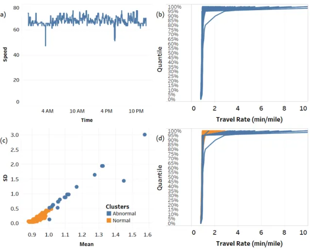
As Lakhina et al. [34] indicated anomalies in network traffic data “are buried like nee-dles in a haystack”. Therefore, from potentially overwhelming massive network-wide traffic, anomaly detection is very challenging. Understanding nature of traffic anomalies is im-portant since they can create unexpected congestion and cause delays in traffic networks. Anomaly detection is crucial from an operational as well as social standpoint. A significant problem with diagnosing anomalies is that their causes can vary considerably. Figure 2 summarizes anomaly detection process. Our overall goal is to be able to detect two types of congestions which are primary reasons of travel rate variability [9, 33]. Hence, we start by clustering days to normal and abnormal categories based on travel rate characteristic (Equation 2). In order to detect abnormal days, first we calculate travel rates percentile values associated to each day’s time series data (Figure 2-b). Since anomalous days have higher variation and are more dynamic as compared to normal days we reduced the di-mension of the distribution to mean and standard deviation. These two features can be further mapped to a two dimensional space (Figure 2-c). Using Local Outlier Factor (LOF) the mean and standard deviation were converted to an density based outlier measurement. This measurement value defines the degree to which a day can be considered an outlier with respect to surrounding neighbors [35]. Since, there is not a certain line (margin) to separate normal traffic rates from anomaly, we utilized Elbow cut off method to determine the anomaly threshold.
With this method we are assuming that the distribution of the two clusters are different. In order to assess the difference we applied Kruskal-Wallis statistical non parametric test [36]. The null hypothesis is that normal and abnormal days are from same distribution and we reject the null hypothesis since calculated p-value for each segment was nearly zero. We argue that anamalous travel rates and as a result atypical traffic behavior can be caused by different types of NRCs. Therefore we mine recurrent pattern associated to normal days d∈D and non-recurrent congestions for anomalous daysd0 ∈D.
T ravelratei∈N = 1 xv s( miles hour ) (2)
Figure 2: Anomaly detection process.
3.3. Denoising the data
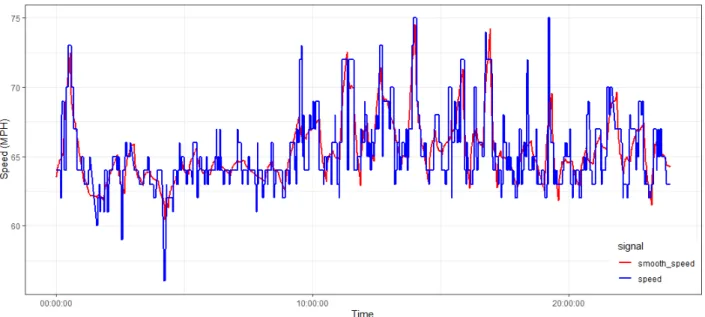
In order to reduce noises in our speed signal and have a robust congestion pattern, we used 1-D denoising with wavelet discrete transform [37]. For discrete signal analysis we used Daubechiesf amily which are compactly supported orthonormal wavelets. The name of Daubechies family is written by dbN where N refers to number of vanishing moments. db2 wavelet transform of Daubechiesf amily with universal Soft threshold [38] and 4 level wavelet decomposition was determined to the most suitable for our application. Figure 3 represents both denoised and original signal values for a specific day.
Figure 3: Denoised and original signal.
3.4. Identifying Appropriate Traffic States Based Upon Speed Values
Detecting abrupt property changes associated with time series data is the main goal of change point detection algorithms. Change point detection has attracted attention of many researchers in data mining and statistics for many years [39]. Change point detection has shown promising application in many fields such as process controlling [40], econometrics [41] , and traffic parameter prediction [42]. Here we intent to apply a change point detection algorithm for traffic state identification.
We first describe mathematical formulation of traffic state detection algorithm. Assume
∀(s, v),{∃ti | xsti,v ∈ Xsv, ptsi,v ∈ Psv, lvs,i ∈ Lvs} Where T = {ti | i ∈ N} denotes the ith
time instant, Pv
s ={ptsi,v | ti ∈ T, v ∈ D, s ∈S} denotes the probability of ith time instant
corresponding to xti,v
s time series (1) , being a change point and Lvs,i = {ls,iv | i ∈ N, v ∈ D, s ∈ S} denotes traffic state change points. For congestion detection, Bayesian change point detection algorithm [43] was applied on each day of the entire year and the change points probabilities Psv = {pti,v
s | ti ∈ T, v ∈ D, s ∈ S} are determined. Later identified
change points probabilities Pv
s ={ptsi,v |ti ∈ T, v ∈ D, s ∈S} are used in (Algorithm 1) in
order to determined traffic state changes points and associated traffic states in (Algorithm 2).
After setting truncate parameter following procedure is used to determine traffic states using probability valuesPv
s ={ptsi,v |ti ∈T, v ∈D, s∈S}. First change points probabilities
Algorithm 1: Determining traffic state change points. Input: Time series probabilities Pv
s
Output: Traffic state change points Lv s,i 1 while i < N do 2 if pti,v s > T hresholdthen 3 for j ←i+ 1 to N do 4 if ptsi,v < T hresholdthen 5 Loc←max{pti,d, . . . , ptj−1,d} 6 lvs,Loc←1 7 break() 8 i←j 9 return Lvs,i
Algorithm 2: Defining Traffic states. Input: Traffic state change points Lv
s,i
Output: Traffic state kti
1 start←1; 2 while i < N do 3 if lvs,i== 1 then
4 Save location of traffic state change point
5 Put data-points from starttoi in the same group
6 start←i+ 1
7 return Kd;
0.01 the max probability was defined as traffic state change point Lvs,i (Algorithm 1). The points before traffic state change point lv
s,i were grouped as one state, having the traffic
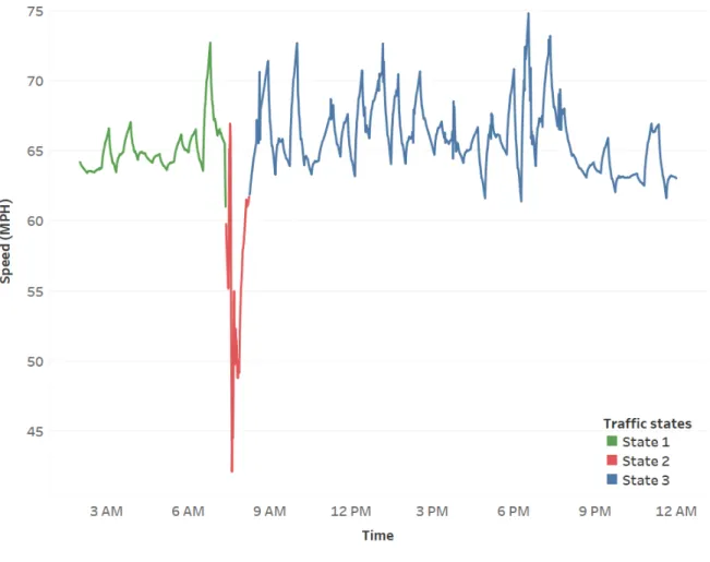
state change point included into that group and this algorithm (Algorithm 2) is repeated for the remaining time instants of a day T ={ti |i ∈N} . It is notable that the primary
conceptual building block of our approach is based on sub-divided road network into multiple smaller segments. There is an extensive large scale time series data set associated to each of these segments, with thousands of daily based recorded data points. Our computations including the change point detection process were massively parallelized, which makes it feasible to apply the whole framework over large networks. Figure 4 shows an example of applying change point detection algorithm on a particular day. As can be seen in Figure 4 by applying change point detection algorithm different traffic stages for a specific date is identified.
Figure 4: Traffic states.
3.5. Congestion detection based on traffic states clustering Consider {tRC
i | i ⊂ N} and {tN RCi | i ⊂ N} where tRCi and tN RCi corresponds to RC
and NRC time instances respectively. After defining traffic states Kd, for each traffic state Kd percentile values (15th,50th,85th) associated with xv,k
s time series have been calculated,
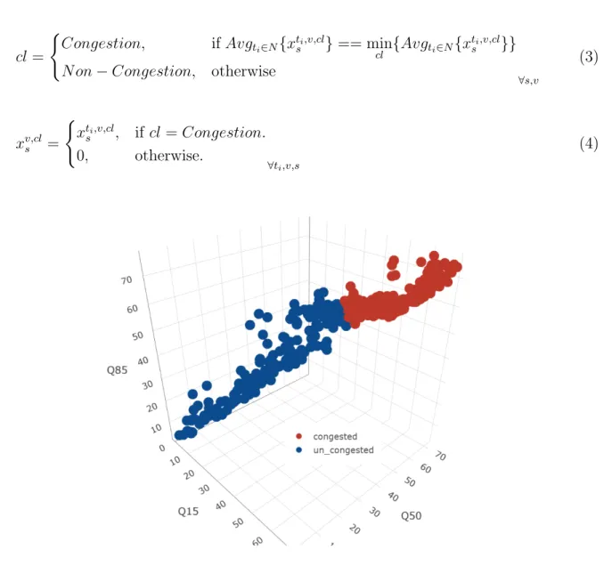
where v ∈ D, k ∈ K, s ∈ S defines date, traffic state, and segment respectively. These percentile values are features for our analysis and since we aim to identify congestion and non-congestion conditions, the number of clusters in this case are predefined (equal 2). Therefore, kmeanclustering algorithm is applied to percentile values for congestion determination and the cluster with the min average speed values is defined as the congestion cluster for each segment (see Figure 5), Formulation (3). It is notable that we are assuming that mining the patterns associated with normal days (d∈D) would illustrate RC. In order to illustrate the effect of signal denoising in the performance of pattern detection, speed profile and congestions condition “heatmaps” for both original and denoised data are presented in Figure 6 . The “heatmap” of congestion pattern is constructed using Formulation (3) and based on modified multivariate time series xv,cls represented in Formulation (4) where v ∈ D,cl
∈ {congestion, non−congestion}, s∈S. cl= ( Congestion, ifAvgti∈N{x ti,v,cl s }== min cl {Avgti∈N{x ti,v,cl s }} N on−Congestion, otherwise ∀s,v (3) xv,cls = ( xti,v,cl s , if cl=Congestion. 0, otherwise. ∀ti,v,s (4)
Figure 5: Congested and non-congested clusters.
As we can see from Figure 6, denoising has helped with removing noises and increased the performance of pattern detection. Moreover, by comparing the speed profiles (real time traffic data) and pattern detection heatmaps resulted from the proposed methodology we can conclude that the proposed methodology is able to capture congestion conditions.
Figure 6: Speed profiles (b & d) and detected congestion patterns (a & c) for original and denoised data respectively.
In order to reduce false-alarm rate and to be able to robustly report the summary statis-tics associated with RC, we utilize elbow cut-off method on the minute-wise congestion percentages. Figure 7 shows elbow curve and minute-wise congestion percentages over the entire year data set after applying elbow cut-off method. As can be seen, there are recurrent patterns starting from 7:16 AM to 8:38 AM and from 4:39 PM to 6:16 PM that associate to morning and evening pick traffic hours respectively. Notably, congestion percentage is calculated based on number of congestion labeled data points divided by total number of data points that correspond to that particular minute, across the entire year for a particular segment.
(a) Elbow curve and cut off point (b) Congestion percentages based on cut-off Figure 7: Elbow cut-off method.
Once we identified time instances that correspond to RCs{tRC
i |i⊂N}based on normal
days performance, in order to identify time instances that corresponds to NRCs{tN RC i |i⊂ N} following steps were taken. Let {t0i ∈N/tRCi | ∀d0 ∈D} &{ti ∈ N/tRCi | ∀d∈ D} then
NRCs time instances{tN RCi |i⊂N} are defined as {tN RCi |i∈ti∪t0i}.
3.6. Delay analysis
Delay was defined as the extra duration taken during the actual travel time with respect to the free flow travel time under the congested regime [44]. Delays were divided into two categories based on the type of congested condition - RC delay and NRC delay. They were calculated based on segments initially and then aggregated for each road and direction. Mathematically, delay for a specific segment Delayh,d
s is defined as in equation 5 in terms
segment, date, hour.
Delaysh,d = P tRC i hT raveltimeds,t i 60 − lengths Ref.speeds i 60 (5)
Wherelengths= length of the segment s in miles,Ref.speedi= reference speed in miles/hour
and T raveltimed
s,i denotes the travel time in minutes. This delay was then converted to a
weighted average for each road and direction based upon the length of the segments. Measuring and reporting the delay as a function of cost has been long prevalent in traffic engineering. This is because of the fact that delay gives an hourly measure and fails to quantify the degree to which slowness is caused due to high volume of traffic. One of the most popular examples of delay cost exploration is carried out by Inrix each year [45]. Delay cost reveals the spatio-temporal characteristics of congestions that can further be utilized in traffic management decisions. We adopt delay cost formulation utilized in [44], where besides delay hours, multiple factors such as Annual Average Daily Traffic (AADT), Monthly Expansion Factor (MEF), and Hourly Volume Portion (HVP) are considered.
4. Results
4.1. Study Location and data
Probe vehicle speed data provided by INRIX with a minute-wise reporting frequency for the entire 2016 calendar year were used in this study [46]. INRIX reports average speed data in one-minute intervals for each segment using on-board GPS devices in vehicles. These on-board devices are used to estimate the real-time speed in freeways and arterial segments. Since the quality of the probe-based data depends on the availability of GPS equipped vehicles, INRIX reports reliability measures (confidence score and c-values). Confidence score takes value 30 when only real time data is used in reporting, while confidence score 20 indicates a mixture of real-time and historical data for reporting, and confidence score 10 is when historical data is reported due to unavailability of probe vehicle. Additional reliability measure is C-value that is reported only if confidence score is 30. This parameter ranges from 0-100 and it is a relative measure for the number of probe-vehicle used in real time speed report. In this study we consider confidence score of 30 that represents real time speed and C-value greater than 30 that has been suggested by Haghani et al. [47]. Developed approach was tested on traffic speed data from Interstate Freeways I-80/35 and I-235 of the Des Moines region, in Iowa, USA, as shown in Figure 8. The Des Moines region experiences the majority of Iowa’s freeway congestion (62% of slow traffic events) along with one of the highest concentrations of traffic incidents within the state [48]. Hence, it is challenging to delevop a reliable decision support system in such a network.
Figure 8: Study region in Des Moines, Iowa.
In this section performance measures including delay hours, and delay costs associated to RC and NRC are analyzed. Total delay hours are color coded by month which allows for
interpretation of potential causes of the congestion and delay. Figure 9 shows total delay hours associated to RC and NRC for each road and month according to the road direction. A majority of total delay hours during June, July, and August is associated to construction while delays during winter months is typically attributed to winter weather. Specifically, the high amount of NRC for I-235 in September is due to incidents.
Figure 9: Monthly total delay hours analysis.
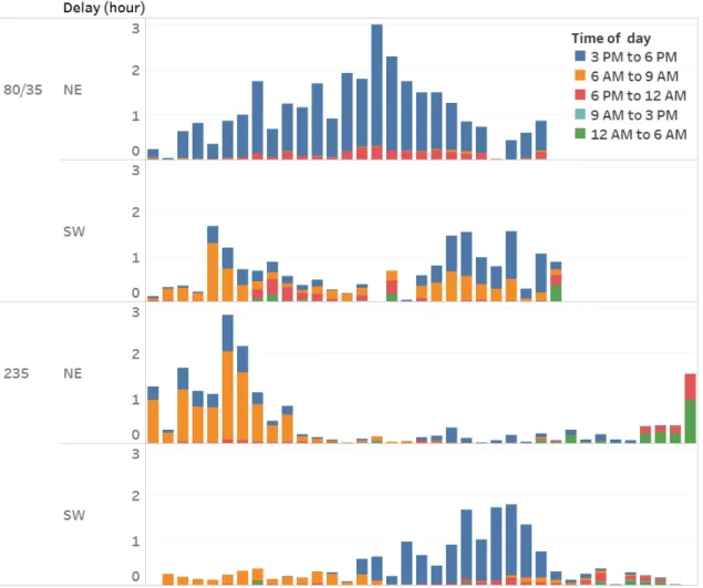
Figure 10 represents RC delays according to time of the day. As shown I-80/35 has morning traffic in South-West direction and evening traffic in North-East direction. While I-235 has morning traffic in North-East direction and evening traffic in South-West direction.
Figure 10: RC delay hours according to time of a day.
Table 1 summarizes delay cost based on type of congestion for each road and road direction. It is notable that the delay cost analysis is based on multiple factors such as truck and vehicle volume, AADT factor and delay hours. As shown in Table 1, I-235 road accounts for around 5 M $ cost of delay in both directions while I-80/35 accounts for 3.5 M $ delay cost.
Table 1: Delay cost analysis.
Type Road Direction RC (M$) NRC (M$) 80/35 S/W 1.03 0.43 N/E 1.82 0.30 235 S/W 2.05 0.39 N/E 1.83 0.50
by the type of congestion. As shown, RC associated with evening pick traffic hours is the main source of delay for I-80/35 north/east direction and I-235 south/ west direction. On the other hand, RC associations to morning traffic pick hours are stronger in I-235 N/E and I-80/35 S/W directions. Figure 11 further reveals that I-235 and I-80/35 interstates have morning and evenings pick traffic hours during 6-9 AM and 3-6 PM, respectively. These results aligne with DOT traffic manager observations which suggests that the proposed methodology accurately captures RC patterns.
Figure 11: Delay hours analysis.
A typical day traffic behavior is presented in Figure 12. The heatmap shows RC con-gestion detection performance of the proposed methodology when x axis is time of the day and y axis is consecutive segments for each road. As shown, the proposed framework is able to detect spatio-temporal RCs which are from 7:30 AM to 8:30 AM and from 3:50 PM to 6:30 PM. These congestion hour periods refer for morning and evening pick traffic hours, respectively. It is notable that in this framework, we are taking advantage of the fact that the capacity reduction due to congestion condition will impact traffic and result in low
speed traffic flow. In this framework the congestion detection methodology is data driven, therefore, entirely relies on speed values. Moreover, it is not based on network parameters such as speed limits and road capacity hence traffic behavior will define congestion. Thus, proposed framework is sensitive to speed changes and for days with high speed traffic flow (unusual but normal traffic flow) that experience abrupt reduction in speed for some dura-tion of a day it will generate a congesdura-tion signal. As by definidura-tion those time segments are congested as compared to normal high speed traffic flow. Those congestion signals based on unusual traffic behavior are shown in Figure 12, I-235 road both North-East and South-West directions in particular segments.
Figure 12: RC heatmap for a given day.
We further did causality analysis on detected NRCs using workzone, incident and weather datasets. The incident and workzone data were obtained from the Traffic Management Center records in Ankeny, Iowa. Data includes location information, start and end time. In this study we tried to connect each detected NRC to these three sources of information according to the time and location. Figure 13 (a) reveals detected NRC that has been
associated with a cause for a given abnormal day across all segments in each road and direction. As shown, during 4 - 5 PM there were a weather condition that affected all road and directions. Moreover, from 12 to 4 AM there was an incident that affected a particular segment in I-235 North-East direction. Figure 13 (b) compares the delay costs associated to detected causes based on each road and direction. Moreover, a statistical interval for delay cost is presented in Figure 13 (c). As shown I-80/35 has a higher average cost and variation as compared to I-235. The results are in alignment with DOT traffic engineers which can present the effectiveness of the proposed methodology. Moreover, This causality analysis can be used for traffic management and investment decisions.
Figure 13: NRC causality profile: (a) associated causes of NRCs for a particular weekday, (b) Total delay cost analysis with respect to causes, (c) Average and standard deviation of delay costs.
We analysed the effect of incidents based on time of the day in Figure 14. As shown in Figure 14 (a), incidents are more happening during night hours (38%). However, incident related cost (b) is highest during 3-6 PM time period and that is due to the fact that within this time period traveler, are generally coming back from work and tired. As a result higher
amount of incident cost (41%). Figure 14 (c) shows total NRC delay in each road-direction. As shown, Most of NRCs in all road and directions are during night hours.
Figure 14: NRC delay profile : (a) Incident induced delay (hour), (b) Incident delay (cost), (c) Percentages of total NRC delay.
Finally we compare the performance of the two roads based on congestion type consid-ering three metrics (delay, cost, and congestion hour) in Figure 15. Since our metrics have different scaling, we compare them based on percentage values. As shown I- 235 has higher congestion hours and NRC delay as compared to I-80/35 which suggests that it is more prone to having bottlenecks. Moreover, due to higher traffic volume of I-235 as compare to I-80/35 it result in higher incident induced delay. Congestion hour defines duration of which congestion has happened but it fails to reveal the severity of congestion. On the other hand delay shows the amount of which each congestion type (RC,NRC) resulted in delay, but again it fails to reveal the severity of congestion and number of vehicles that have been affected by the congestion. In order to illustrade the severity of congestion in terms of delay hours and number of vehicle that have been affected by the congestion we consider the delay cost in the analysis. Since I-80/35 has a higher average number of trucks it has
higher amount of total delay. On the other hand since, I-235 has higher vehicle volume, higher number of vehicles get affected by congestion condition (social and emission cost). Thereby congestion resulted in higher cost value as compared to I-80/35.
Figure 15: Performance measure comparison.
5. Conclusion
In this study a highly parallelized and systematic data driven framework for identifying freeway’s RC and NRCs have been presented. The presented framework leverages wealthy historical data and it is self adaptive to any data set, to further uncover the spatiotemporal RC and NRCs. Most existing work in congestion detection literature considers incidents as the main cause of NRC and connects NRC directly to incidents. However, in this study we leverage wealthy historical data to guide us in identifying congestion patterns. The proposed
data driven framework is not limited to a specific or additional data set (e.g., incidents) to identify NRCs. Therefore it addresses the limits of prior work in congestion detection. In order to increase the true positive rate a sensitive traffic state detection algorithm was intro-duced. Meanwhile, in order to reduce the false alarm rate due to traffic variable fluctuations, the following procedure was implemented: 1- input signal was temporally denoised, 2- an elbow cut-off method was applied on the minute-wise congestion probabilities such that the time instances below cut-off threshold were removed temporally from RC pattern. By comparing the raw speed profile with detected congestion pattern, we can conclude that the proposed analytical framework is able to detect spatio-temporal congestion accurately. Moreover, it is self adaptive to new data-sets and it does not rely on any data-set or spe-cific characteristics of the data set to detect spatio-temporal congestion. We analyzed the performance measures of congestion for each road including delay and delay cost and we further associated the detected NRCs to their causes based on work zone, weather and inci-dent data-sets. In addition to the insights extracted from the data-set, the proposed system intends to be a valuable support for traffic management in tactical and strategic decisions.
References
[1] I. Statistics, CO2 emissions from fuel combustion-highlights, IEA, Paris http://www. iea. org/co2highlights/co2highlights. pdf. Cited July .
[2] R. Joumard, P. Jost, J. Hickman, D. Hassel, Hot passenger car emissions modelling as a function of instantaneous speed and acceleration, Science of the Total Environment 169 (1-3) (1995) 167–174. [3] N. Owens, A. Armstrong, P. Sullivan, C. Mitchell, D. Newton, R. Brewster, T. Trego, Traffic incident
management handbook, Tech. Rep., 2010.
[4] D. Schrank, B. Eisele, T. Lomax, J. Bak, 2015 urban mobility scorecard .
[5] K. Ozbay, P. Kachroo, Incident management in intelligent transportation systems .
[6] R. Dowling, A. Skabardonis, M. Carroll, Z. Wang, Methodology for measuring recurrent and nonrecur-rent traffic congestion, Transportation Research Record 1867 (1) (2004) 60–68.
[7] L. D. Han, A. D. May, Automatic detection of traffic operational problems on urban arterials, Tech. Rep., 1989.
[8] J. Kwon, M. Mauch, P. Varaiya, Components of congestion: Delay from incidents, special events, lane closures, weather, potential ramp metering gain, and excess demand, Transportation Research Record 1959 (1) (2006) 84–91.
[9] R. B. Noland, J. W. Polak, Travel time variability: a review of theoretical and empirical issues, Trans-port reviews 22 (1) (2002) 39–54.
[10] H.-Y. Cheng, V. Gau, C.-W. Huang, J.-N. Hwang, Advanced formation and delivery of traffic informa-tion in intelligent transportainforma-tion systems, Expert Systems with Applicainforma-tions 39 (9) (2012) 8356–8368. [11] L. Calderoni, D. Maio, S. Rovis, Deploying a network of smart cameras for traffic monitoring on a “city
kernel”, Expert Systems with Applications 41 (2) (2014) 502–507.
[12] W. Wen, An intelligent traffic management expert system with RFID technology, Expert Systems with Applications 37 (4) (2010) 3024–3035.
[13] S. Kamran, O. Haas, A multilevel traffic incidents detection approach: Identifying traffic patterns and vehicle behaviours using real-time gps data, in: 2007 IEEE Intelligent Vehicles Symposium, IEEE, 912–917, 2007.
[14] J. Bacon, A. I. Bejan, A. R. Beresford, D. Evans, R. J. Gibbens, K. Moody, Using real-time road traffic data to evaluate congestion, in: Dependable and Historic Computing, Springer, 93–117, 2011.
[15] J. Yoon, B. Noble, M. Liu, Surface street traffic estimation, in: Proceedings of the 5th international conference on Mobile systems, applications and services, ACM, 220–232, 2007.
[16] M. E. Hallenbeck, J. Ishimaru, J. Nee, et al., Measurement of recurring versus non-recurring congestion, Tech. Rep., Washington (State). Dept. of Transportation, 2003.
[17] T. Thomas, E. C. van Berkum, Detection of incidents and events in urban networks, IET Intelligent Transport Systems 3 (2) (2009) 198–205.
[18] A. Skabardonis, P. Varaiya, K. F. Petty, Measuring recurrent and nonrecurrent traffic congestion, Transportation Research Record 1856 (1) (2003) 118–124.
[19] R. Yu, Y. Lao, X. Ma, Y. Wang, Short-term traffic flow forecasting for freeway incident-induced delay estimation, Journal of Intelligent Transportation Systems 18 (3) (2014) 254–263.
[20] J. Li, C.-J. Lan, X. Gu, Estimation of incident delay and its uncertainty on freeway networks, Trans-portation research record 1959 (1) (2006) 37–45.
[21] Z. Chen, X. C. Liu, G. Zhang, Non-recurrent congestion analysis using data-driven spatiotemporal approach for information construction, Transportation Research Part C: Emerging Technologies 71 (2016) 19–31.
[22] J. E. Moore, G. Giuliano, S. Cho, Secondary accident rates on Los Angeles freeways, Journal of Trans-portation Engineering 130 (3) (2004) 280–285.
[23] M.-I. M. Imprialou, F. P. Orfanou, E. I. Vlahogianni, M. G. Karlaftis, Methods for defining spatiotem-poral influence areas and secondary incident detection in freeways, Journal of transportation engineering 140 (1) (2013) 70–80.
detection on urban road networks, Transportation Research Part C: Emerging Technologies 48 (2014) 47–65.
[25] Y. Chung, W. W. Recker, A methodological approach for estimating temporal and spatial extent of delays caused by freeway accidents, IEEE Transactions on Intelligent Transportation Systems 13 (3) (2012) 1454–1461.
[26] Y. Chung, Quantification of nonrecurrent congestion delay caused by freeway accidents and analysis of causal factors, Transportation research record 2229 (1) (2011) 8–18.
[27] M. Snelder, T. Bakri, B. van Arem, Delays caused by incidents: Data-driven approach, Transportation research record 2333 (1) (2013) 1–8.
[28] B. Anbaro˘glu, T. Cheng, B. Heydecker, Non-recurrent traffic congestion detection on heterogeneous urban road networks, Transportmetrica A: Transport Science 11 (9) (2015) 754–771.
[29] E. D’Andrea, F. Marcelloni, Detection of traffic congestion and incidents from GPS trace analysis, Expert Systems with Applications 73 (2017) 43–56.
[30] Y. Chung, Assessment of non-recurrent congestion caused by precipitation using archived weather and traffic flow data, Transport Policy 19 (1) (2012) 167–173.
[31] Y. Chung, Assessment of non-recurrent traffic congestion caused by freeway work zones and its statis-tical analysis with unobserved heterogeneity, Transport Policy 18 (4) (2011) 587–594.
[32] F. Habtemichael, M. Cetin, K. Anuar, Methodology for quantifying incident-induced delays on freeways by grouping similar traffic patterns, in: Transportation Research Board 94th Annual Meeting, 15–4824, 2015.
[33] A. R. G¨uner, A. Murat, R. B. Chinnam, Dynamic routing under recurrent and non-recurrent congestion using real-time ITS information, Computers & Operations Research 39 (2) (2012) 358–373.
[34] A. Lakhina, M. Crovella, C. Diot, Mining anomalies using traffic feature distributions, in: ACM SIG-COMM computer communication review, vol. 35, ACM, 217–228, 2005.
[35] M. M. Breunig, H.-P. Kriegel, R. T. Ng, J. Sander, LOF: identifying density-based local outliers, in: ACM sigmod record, vol. 29, ACM, 93–104, 2000.
[36] W. H. Kruskal, W. A. Wallis, Use of ranks in one-criterion variance analysis, Journal of the American statistical Association 47 (260) (1952) 583–621.
[37] O. Rioul, M. Vetterli, Wavelets and signal processing, IEEE signal processing magazine 8 (ARTICLE) (1991) 14–38.
[38] D. L. Donoho, De-noising by soft-thresholding, IEEE transactions on information theory 41 (3) (1995) 613–627.
[39] M. Basseville, I. V. Nikiforov, et al., Detection of abrupt changes: theory and application, vol. 104, Prentice Hall Englewood Cliffs, 1993.
[40] L. A. Aroian, H. Levene, The effectiveness of quality control charts, Journal of the American Statistical Association 45 (252) (1950) 520–529.
[41] J. Chen, A. K. Gupta, Testing and locating variance changepoints with application to stock prices, Journal of the American Statistical association 92 (438) (1997) 739–747.
[42] G. Comert, A. Bezuglov, An online change-point-based model for traffic parameter prediction, IEEE Transactions on Intelligent Transportation Systems 14 (3) (2013) 1360–1369.
[43] R. P. Adams, D. J. MacKay, Bayesian online changepoint detection, arXiv preprint arXiv:0710.3742 . [44] 2016 Interstate Congestion in Iowa — Iowa Department of Transportation - Open Data,
https://data.iowadot.gov/datasets/2016-interstate-congestion-in-iowa, (Accessed on 09/29/2019), ????
[45] Scorecard - INRIX,http://inrix.com/scorecard/, (Accessed on 09/30/2019), ???? [46] INRIX, 2016.
[47] A. Haghani, M. Hamedi, K. F. Sadabadi, I-95 Corridor coalition vehicle probe project: Validation of INRIX data, I-95 Corridor Coalition 9.