Tractable POMDP-planning for robots with complex non-linear dynamics

(1)

Tractable POMDP-planning for robots with

complex non-linear dynamics

Marcus Hoerger

Dipl.-Inf.

https://orcid.org/0000-0002-4698-5875

A thesis submitted for the degree of Doctor of Philosophy at

The University of Queensland in 2020

(2)

Planning under partial observability is an essential capability of autonomous robots. While robots operate in the real world, they are inherently subject to various uncertainties such a control and sensing errors, and limited information regarding the operating environment. Conceptually these type of planning problems can be solved in a principled manner when framed as a Partially Observable Markov Decision Process (POMDP). POMDPs model the aforementioned uncertainties as conditional probability functions and estimate the state of the system as probability functions over the state space, called beliefs. Instead of computing the best strategy with respect to single states, POMDP solvers compute the best strategy with respect to beliefs. Solving a POMDP exactly is computationally intractable in general.

However, in the past two decades we have seen tremendous progress in the development of approximately optimal solvers that trade optimality for computational tractability. Despite this progress, approximately solving POMDPs for systems with complex non-linear dynamics remains challenging. Most state-of-the-art solvers rely on a large number of expensive forward simulations of the system to find an approximate-optimal strategy. For systems with complex non-linear dynamics that admit no closed-form solution, this strategy can become prohibitively expensive. Another difficulty in applying POMDPs to physical robots with complex transition dynamics is the fact that almost all implementations of state-of-the-art on-line POMDP solvers restrict the user to specific data structures for the POMDP model, and the model has to be hard-coded within the solver implementation. This, in turn, severely hinders the process of applying POMDPs to physical robots.

In this thesis we aim to make POMDPs more practical for realistic robotic motion planning tasks under partial observability. We show that systematic approximations of complex, non-linear transition dynamics can be used to design on-line POMDP solvers that are more efficient than current solvers. Furthermore, we propose a new software-framework that supports the user in modeling complex planning problems under uncertainty with minimal implementation effort.

(3)

Declaration by author

This thesis is composed of my original work, and contains no material previously published or written by another person except where due reference has been made in the text. I have clearly stated the contribution by others to jointly-authored works that I have included in my thesis.

I have clearly stated the contribution of others to my thesis as a whole, including statistical assistance, survey design, data analysis, significant technical procedures, professional editorial advice, financial support and any other original research work used or reported in my thesis. The content of my thesis is the result of work I have carried out since the commencement of my higher degree by research candidature and does not include a substantial part of work that has been submitted to qualify for the award of any other degree or diploma in any university or other tertiary institution. I have clearly stated which parts of my thesis, if any, have been submitted to qualify for another award.

I acknowledge that an electronic copy of my thesis must be lodged with the University Library and, subject to the policy and procedures of The University of Queensland, the thesis be made available for research and study in accordance with the Copyright Act 1968 unless a period of embargo has been approved by the Dean of the Graduate School.

I acknowledge that copyright of all material contained in my thesis resides with the copyright holder(s) of that material. Where appropriate I have obtained copyright permission from the copyright holder to reproduce material in this thesis and have sought permission from co-authors for any jointly authored works included in the thesis.

(4)

1. [1]M. Hoerger, H. Kurniawati and A. Elfes, Multilevel Monte-Carlo for Solving POMDPs Online, in: Proc. International Symposium on Robotics Research (ISRR) (To Appear), 2019 2. [2]M.Hoerger, J. Song, H.Kurniawati and A. Elfes, POMDP-based Candy Server: Lessons

Learned From a Seven Day Demo, in: Proc. AAAI International Conference on Autonomous Planning and Scheduling (ICAPS), 2019, pp. 698-706

3. [3]M. Hoerger, H. Kurniawati, and A. Elfes, A Software Framework for Planning under Partial Observability. in: Proc. IEEE/RSJ International Conference on Intelligent Robots and Systems (IROS), 2018, pp. 7576-7582

4. [4]M. Hoerger, H. Kurniawati, T. Bandyopadhyay and A. Elfes, Linearization in Motion Plan-ning under Uncertainty, in: Proc. 12th International Workshop on the Algorithmic Foundations of Robotics (WAFR), 2016.

Submitted manuscripts included in this thesis

No manuscripts submitted for publication.

Other publications during candidature

1. [5]M. Hoerger, H. Kurniawati, T. Bandyopadhyay, and A. Elfes, Effects of Obstacle Avoidance to LQG-Based Motion Planners, in: Australasian Conference on Robotics and Automation, ARAA, 2016

2. [6] A. Snoswell, V. Dewanto,M. Hoerger, H. Kurniawati and S. Singh, A Distributed, Any-Time Robot Architecture for Robust Manipulation, in: Australasian Conference on Robotics and Automation, ARAA, 2018

3. [7] A. Elfes, R. Steindl, F. Talbot, F. Kendoul, P. Sikka, T. Lowe, N. Kottege, M. Bjelonic, R. Dungavell, T. Bandyopadhyay andM. Hoerger, The Multilegged Autonomous eXplorer (MAX), in: Proceedings of the IEEE International Conference on Robots and Automation (ICRA), 2017

Contributions by others to the thesis

• Dr. Hanna Kurniawati and Dr. Alberto Elfes guided and supported me through my candidature. This included the conception of the problem and substantial help in writing the publications that were generated during this candidature, particular for the earlier publications.

(5)

• Joshua Song designed and implemented the perception system for the Kinova MOVO mobile manipulator that was used for the experiments in Chapter 4.

• Aaron Snoswell and Vektor Devanto implemented the low-level system architecture for the Kinova MOVO mobile manipulator that was used for the experiments in Chapter 4

Statement of parts of the thesis submitted to qualify for the award

of another degree

No works submitted towards another degree have been included in this thesis.

Research involving human or animal subjects

No animal or human subjects were involved in this research.

(6)

First and foremost, I want to express my sincere gratitude to my principal advisor Dr. Hanna Kurniawati for her tremendous guidance throughout this journey. Her seemingly endless patience and ongoing support has helped me to grow as a researcher and professional on all levels. Without Hanna’s leadership and advice this thesis would have not been possible.

Furthermore, I am grateful for Dr. Alberto Elfes to serve as my co-advisor. Alberto not only became an advisor, but a mentor and leader who keeps on inspiring me and countless other people. Alberto is the one who encouraged me to pursue a PhD program after working as a research intern within CSIRO’s Robotics and Autonomous Systems Group. Thank you for granting me this amazing opportunity and making my PhD candidature possible in the first place.

Within UQ’s School of ITEE, I want to thank my Confirmation and Review Committee for their time spent on assessing my candidature and providing valuable feedback. A special thank you goes to the Chair of the Committee Dr. Surya Singh. He always had an open ear for research related questions and granted valuable time for presentation rehearsals and interesting discussions. Thank you also to ITEE’s HDR Liaison Officer Tracey Miller and all the people at the Graduate School for their support with administrative related tasks.

I thank all the great people I have met within CSIRO’s Robotics and Autonomous Systems Group, particularly Dr. Navinda Kottege who supported me in securing a UQI International Student and CSIRO Postgraduate Student scholarship. Thank you to Dr. Tirthankar Bandyopadhyay for your advice and for being a great colleague.

Outside the professional domain I want to thank my mother Eva Hoerger and my sister Natascha Hoerger for being a major pillar in my life, for their tremendous personal support, and for providing a safe haven. Thank you to all my friends back home in Germany and the countless new friends I’ve met while staying in Australia. You provided a place for me to retreat, relax and enjoy life outside the lab.

Last but not least, I want to thank my dad Dieter Hoerger, who unfortunately passed away during this candidature. Thank you for always believing in me, supporting me in all my decisions and for being proud of me.

(7)

Financial support

This research was supported by the University of Queensland International Scholarship (UQI) and the CSIRO Postgraduate Studentship.

Keywords

partially observable markov decision process, pomdp, motion planning under uncertainty, modelling, control

Australian and New Zealand Standard Research Classifications

(ANZSRC)

ANZSRC code: 010303, Optimisation, 40%

ANZSRC code: 080110, Simulation and Modelling, 40% ANZSRC code: 080306, Open Software, 20%

Fields of Research (FoR) Classification

FoR code: 0103, Numerical and Computational Mathematics, 40% FoR code: 0801, Artificial Intelligence and Image Processing, 40% FoR code: 0803, Computer Software, 20%

(8)

List of Figures

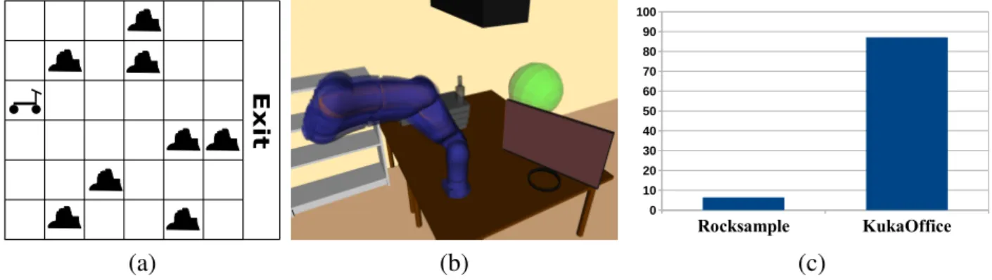
1.1 Illustration of a belief tree. The nodes represent beliefs. Every node has|A| outgoing edges that represent actions. These actions branch into|Z|observations. The root of the tree represents the initial beliefb₀. . . 5 1.2 (a) An instance of the Rocksample problem, a common benchmark problem for

on-line POMDP solvers. (b) The manipulator problem, where a 7DOFs torque-controlled manipulator has to reach a goal area (green sphere) with its end-effector, while being subject to control and observation errors. Blue particles represent samples from the belief. (c) Percentage of the total planning time (CPU time) used by ABT to perform the forward-simulations during policy computation in both problems. . . 6

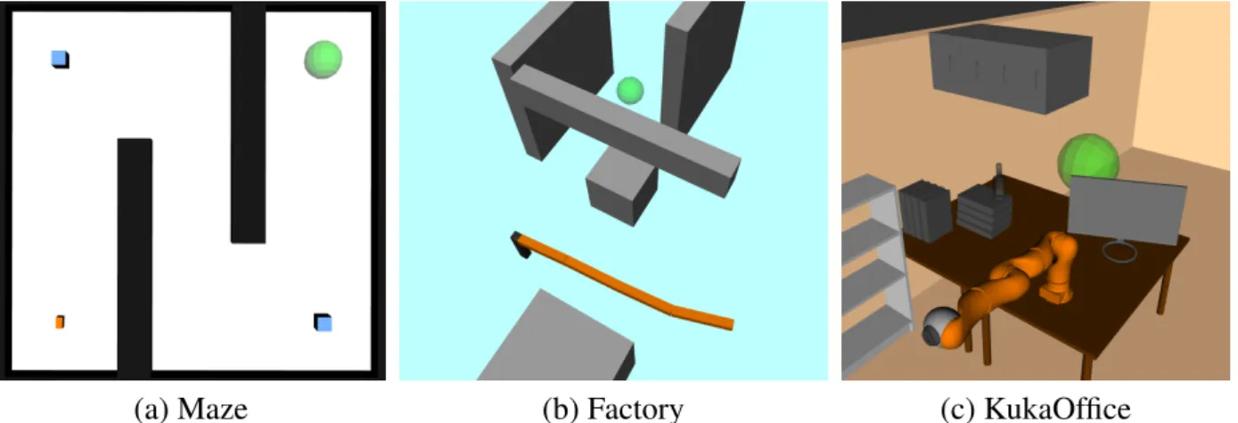
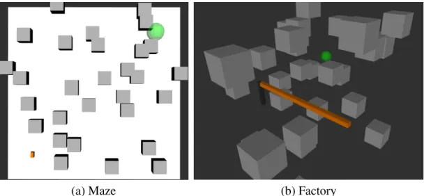
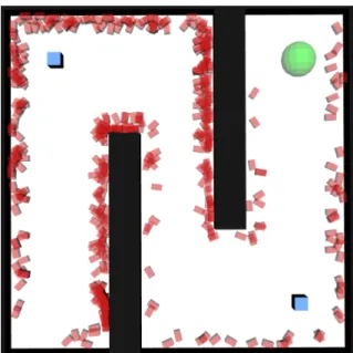
2.1 Test scenarios for the different robots. The objects colored black and gray are obstacles, while the green sphere is the goal region. (a) The Maze scenario for the car-like robot. The blue squares represents the beacons, while the orange square at the bottom left represents the initial state. (b) The 4DOFs-manipulator scenario. (c) The KukaOffice scenario . . . 24 2.2 The average total discounted rewards achieved by ABT and MHFR in the Maze scenario,

as the uncertainties increase. Vertical bars are the 95% confidence intervals. . . 25 2.3 Two example scenarios for the Car-like robot (a) and the 4DOFs-manipulator (b) with 30

randomly distributed obstacles. . . 27 2.4 State samples (shown in red) in the Maze scenario for which the approximated SNM value

exceeds the chosen threshold of 0.51 . . . 30

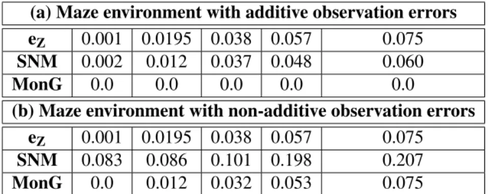
3.1 Test scenarios used to evaluate MLPP. (a)Factory(b)KukaOffice(c)CarNavigation (d)MovoGrasping . . . 42 3.2 Average variance ofQ_l(solid blue line) andQ_l−Q_l−₁(dashed red line) for the problem

scenarios (a) Factory, (b) KukaOffice, (c) CarNavigation and (d) MovoGrasping. The

x-axis represents the levell, whereas they-axis represents the variance. . . 46 x

(11)

LIST OF FIGURES xi 3.3 Average total discounted reward of MLPP, ABT and POMCP on theFactory(a),KukaOffice

(b),CarNavigation(c) andMovoGrasp(d) scenarios. Thex-axis represents the level of approximation of the transition function used for planning. Note that MLPP uses all levels for planning (hence the horizontal lines), whereas ABT and POMCP use only a single level as indicated by thex-axis. For each scenario, the largest level of approximation is equal to the original transition function. Vertical bars are the 95% confidence intervals. . 47 3.4 Average total discounted rewards for ABT, POMCP and MLPP forFactoryusing

in-creasing planning times per step. The average is taken over 500 simulation runs for each planning time and algorithm. Vertical bars are the 95% confidence intervals. . . 48 4.1 OPPT architecture overview. Rounded boxes represent core components of the OPPT

framework. Square-shaped boxes represent components for which alternative implementa-tions can be provided. A directed arrow from A to B depicts ”A is owned by B” . . . 53 4.2 The problem scenario for the CandyScooper problem. A MOVO mobile manipulator

equiped with a 6DOFs Jaco arm with KG3 gripper must pick-up at cup located on a table in front of the robot, use the cup to scoop candy from a candy box located next to the table, and put the cup back on the table. . . 58 4.3 (a) and (b): Finite state machines of the macro-actions. Ovals are machine-states, labeled

solid arrows are actions, dashed arrows are observations, and double circles are exit states.

o_{ob j} are observations with respect to the pose of the cup, whereaso_graspare observation from the grasping sensor. . . 64 4.4 These figures show snapshots of a successful run with two obstacle position changes. Here

the robot attempts to pick-up the cup (first picture) but the cup position is changed to the left corner of the table (second picture). It performs ascanaction, and the robot attempts to pick up the cup again. But, as the robot attempts to pick-up the cup at the new position, the cup is again moved to a location close to the robot (third picture). Ascanaction is performed again. In the last picture the robot successfully picks-up the cup at its the new location. . . 68 4.5 The problem scenario used for the set of experiments with one (a) and three (b) obstacles.

The task for the robot is pick-up the cylindrical cup while avoiding collisions with the two boxes and the black cup. . . 69

(12)

List of Tables

2.1 Average values of SNM, MonG and the relative value difference between ABT and MHFR for the 4DOFs-manipulator (a) and the car-like robot (b) operating inside empty

environments. . . 24

2.2 Average values of SNM, MonG and the relative value difference between ABT and MHFR for the 4DOFs-manipulator operating inside the Factory environment (a) and the car-like robot operating inside the Maze environment (b). . . 25

2.3 Average values of SNM, MonG and the relative value difference between ABT and MHFR for the 4DOFs-manipulator operating inside the Factory environment (a) and the car-like robot operating inside the Maze environment (b) while being subject to collision dynamics. 26 2.4 Average values of SNM, MonG and relative value difference between ABT and MHFR for the 4DOFs-manipulator (a) and the car-like robot (b) operating inside environments with increasing numbers of obstacles. hereeT =eZ =0.038. . . 27

2.5 Comparison between the observation component of SNM and MoNG for the 4DOF-manipulator operating inside the Factory environment with observation function eq.(2.21) (a) and eq.(2.26) (b) . . . 28

2.6 Comparison between the observation component of SNM and MoNG for the car-like robot operating inside the Maze environment with observation function eq.(2.23)(a) and observation function eq.(2.27)(b) . . . 28

2.7 Average values of SNM, MonG and the relative value difference between ABT and MHFR for the 4DOFs-manipulator operating inside the Factory environment (a) and the car-like robot operating inside the Maze environment (b) with non-additive observation errors . . 29

2.8 Average total discounted reward and±95% confidence interval over 100 simulation runs. Heree_T =pez=0.038 for all scenarios. The proportion of ABT being used in the Maze, Factory and Office scenarios is 37.85%, 56.43% and 42.33% respectively. . . 30

4.1 Main classes of OPPT and their respective core methods . . . 53

4.2 State and observation configuration variables for motion planning problems . . . 55

4.3 Action configuration variables for motion planning problems . . . 56

4.4 Percentage of successful runs for scenarios with 0, 2, 4, and 6 cup position changes. For each scenario the robot performed 20 execution runs . . . 69

(13)

Chapter 1 Introduction

Motion planning under partial observability is both challenging and essential for autonomous robots. To operate reliably, an autonomous robot must act strategically to accomplish its task, despite being subject to various types of uncertainties, such as motion, actuation and sensing uncertainty and uncertainty regarding the environment the robot operates in. Due to these uncertainties, the robot does not have full observability of its state and/or the state of its operating environment. Conceptually, this problem can be solved in a systematic and principled manner when framed as the Partially Observable Markov Decision Process (POMDP) [8]. A POMDP represents the aforementioned uncertainties as conditional probability functions, and estimates the state of the system (following a sequence of actions and observations that the robot has performed and perceived) as probability distributions over the state space, calledbeliefs. Solving a POMDP constitutes of systematically reasoning over the belief spaceB, the set of all probability distributions over the state space, by taking into account the various uncertainties the robot is subject to. The robot then chooses the optimal strategy with respect to beliefs rather than single states in order to maximize its expected long-term outcome. Unfortunately, solving a POMDP exactly is computationally intractable in general [9], even for 3DOFs point robots [10, 11]. In particular the size ofBgrows exponentially with the size of the state space (”curse of dimensionality”) and the number of possible strategies grows doubly exponential with the planning horizon (”curse of history”). Due to these computational challenges, POMDPs have often been considered impractical for all but the simplest problems.

However, in the past two decades we have seen tremendous progress in the development of approximate POMDP solvers that trade optimality for computational tractability. The underlying principle of these methods is the fact that in many applications a near-optimal strategy is ”good enough” to accomplish a given task. Several general approximate POMDP solvers —that do not restrict the type of dynamics and sensing model of the system, nor the type of distributions used to represent uncertainty— can now compute good motion strategies on-line with a 1-10Hz update rate for a number of robotic problems [12–15]. Despite these advances, applying state-of-the-art approximate POMDP solvers to realistic robotic systems remains challenging. These systems often have a large number of degrees-of-freedom (DOFs) and complex, non-linear transition dynamics, causing the efficiency of

(14)

current POMDP solvers to degrade rapidly. To find a good strategy, most today’s solvers simulate the effect of many sequences of actions from different beliefs. A simulation run generally requires expensive numerical integrations, and complex transition dynamics tend to increase the cost of each numerical integration, which in turn significantly increases the total planning cost. Of course, this cost increases rapidly for problems that require more or longer simulation runs, such as in problems with long planning horizons.

As a computationally attractive alternative to general POMDP-planning, various methods have been developed that extend algorithms from sampling-based deterministic motion planning to the stochastic domain. These methods typically simplify planning in the belief space by imposing restrictions on the type of systems and class of beliefs, which in turn speeds up the planning process. However, it is not clear how these problem simplifications affect the quality of the resulting motion strategies.

Another challenge in applying POMDPs to physical robots with complex transition dynamics is the fact most (if not all) implementations for state-of-the-art solvers restrict the user to specific data structures for the POMDP model, or the model has to be hard-coded within the solver implementation. This, in turn, severely hinders the process of applying POMDPs to physical robots.

In this thesis we aim to make POMDPs more practical for realistic robotic motion planning tasks under partial observability. We show that systematic approximations of complex, non-linear transition dynamics can be used to design on-line POMDP solvers that are more efficient than current state-of-the-art solvers. Furthermore, we propose a new software-framework which supports the user in modeling complex planning problems under partial observability with minimal implementation effort.

In this chapter we present a brief introduction to motion planning under uncertainty algorithms and discuss their shortcomings in Section 1.1. We then present a formal introduction to POMDPs Section 1.2, followed by a brief overview of POMDP solvers, with a focus on on-line solvers in Section 1.3. In Section 1.4 we discuss the limitations of on-line POMDP solvers for systems with complex, non-linear transition dynamics before providing an overview of our main contributions in Section 1.5. Finally, the remainder of this thesis is outlined in Section 1.6.

1.1 Motion Planning under Uncertainty

To reduce the complexity of planning in the belief space, several motion planning under uncertainty algorithms have been proposed that reap from the success of probabilistic sampling-based algorithms for deterministic problems, such as Probabilistic Roadmap (PRM) [16], Rapidly-Exploring-Random-Tree (RRT) [17] variants thereof [18, 19]. These algorithms enabled solving motion planning problems involving robots with many degrees-of-freedom that were deemed too difficult to solve with traditional methods, such as grid-search-based methods [20, 21].

To lift the planning problem from the state space to the belief space, Stochastic Roadmap [22] combines PRM with the Markov Decision Process (MDP) [23], a special class of POMDP that assumes the state of the robot is fully observable. Due to the use of MDP, this method cannot handle partial observability. The Belief Roadmap [24] can handle partial observability, but restricts the robot’s

(15)

1.2. PARTIALLY OBSERVABLE MARKOV DECISION PROCESS (POMDP) 3 transition and observation dynamics to be linear(ized) and the beliefs to be Gaussian distributions. More recently methods have been proposed that formulate the belief space planning problem as a stochastic control problem: LQG-MP [25] combines RRT with a Linear-Quadratic-Gaussian (LQG) feedback-controller [26]. It samples a finite set of trajectories using RRT and uses an LQG-controller to follow the trajectory that minimizes an expected quadratic cost function. FIRM [27] extends PRM to the belief space and constructs independent LQG-controllers for each node. HFR [28] is an on-line variant of LQG-MP. Similar to LQG-MP, HFR uses RRT to sample a set trajectories that are evaluated in belief space, but does so at each planning step. In contrast to methods that extend deterministic sampling-based motion planning algorithms to belief space planning, [29] starts from a nominal trajectory that is iteratively modified using sequential quadratic programming [30] to minimize a cost function, assuming maximum likelihood observations.

Note that although these methods don’t address the general POMDP problem, they can be seen as a special class of POMDP solvers for motion planning under uncertainty problems. We will therefore refer to them aslinearization-based POMDP solvers.

A common limitation of this class of solvers (except for Stochastic Roadmap, which cannot handle partial observability), is the fact that they rely on linear(ized) system and observation dynamics and assume that beliefs can be represented as Gaussian distributions. However, it is known that linearization only works well for systems with ”mild” [31] non-linearities. Additionally, for robots operating in cluttered environments or in the vicinity of dynamic constraints, Gaussian distributions can be inadequate to accurately model beliefs. Even though computationally more complex, POMDP solvers don’t suffer from these limitations.

1.2 Partially Observable Markov Decision Process (POMDP)

The Partially Observable Markov Decision Process is a principled mathematical framework to model and solve motion planning problems under partial observability. Formally a POMDP is a tuple

<S,A,O,T,Z,R,γ >, whereS,AandOare the state, action and observation spaces of the robot. T andZ model the uncertainty in the effect of taking actions and receiving observations as conditional probability functionsT(s,a,s0) =p(s0|s,a)andZ(s0,a,o) = p(o|s0,a), wheres,s0∈S,a∈Aando∈O.

R(s,a) models the reward the robot receives when performing action a fromsand 0<γ <1 is a discount factor. Due to uncertainties in the effect of actions and receiving observations, the true state of the robot is only partially observable. Hence, instead of planning with respect to states, the robot has to plan with respect to probability distributionsb∈Bover the state space, called beliefs, whereB, called the belief space, is the set of all probability distributions overS. The solution of a POMDP is an optimal policyπ∗, a mapping from beliefs to actionsπ∗:b7→a∈Asuch that the robot maximizes the expected discounted future reward when followingπ∗,i.e.

E " ∞

∑

t=0 γtrt # (1.1)

(16)

wherer_t is the reward received at timet. Onceπ∗has been computed, it can be used as a feedback-controller: Given the current beliefb, the robot performsπ∗(b), receives an observationo∈Oand updates its belief according tob0=τ(b,a,o), such that

b0(s0) =τ(b,a,o)(s0) =ηZ(s0,a,o) Z s∈S T(s,a,s0)b(s)ds (1.2) whereη=1/ R_s0_∈SZ(s0,a,o)R_s∈ST(s,a,s0)dsds0

is a normalization constant. The value achieved by a policyπ at a particular beliefbcan be compactly expressed as

V_π(b) =R(b,π(b)) +γ Z o∈O Z(b,π(b),o)Vπ(τ(b,π(b),o))do (1.3) where R(b,a) =R s∈SR(s,a)b(s)ds and Z(b,a,o) = R s0∈SZ(s0,a,o) R s∈ST(s,a,s0)b(s)dsds0. The value achieved by the optimal policyπ∗is then the policy that satisfiesπ∗(b) =arg max_πVπ(b).

1.3 POMDP Solvers

POMDP solvers have seen tremendous advances in the past two decades. The key of their success is the use of sampling to trade optimality for computational tractability. Instead of computing a policy for the entire belief space, sampling based planners representBby a set of sampled beliefs and compute the policy for this sampled set only. In general there are two classes of POMDP solvers: Off-line an on-line solvers. Off-line solvers compute a policy a-priori which is then executed during run-time. These solvers (e.g.[32–36]) typically use a point based approach to compute the value function at a representative set of sampled beliefs.

In contrast to off-line solvers, on-line solvers interleave policy computation and policy execution. They search for a single best action for the current belief only, execute the action and update the belief. This process then repeats from the new belief. By computing a policy with respect to the current belief only, on-line POMDP solvers usually scale much better to larger problems [37]. Hence, in this thesis, we are primarily focusing on on-line solvers.

To compute a policy for the current belief, on-line solvers typically construct and evaluate a belief tree using lookahead search. A belief tree is a set of nodes, representing beliefs, that are connected via action-observation edges, such that a beliefb0is a child ofbvia edge(a,o)ifb0=τ(b,a,o). The root of the belief tree represents the initial belief. An illustration of a belief tree is shown in Figure 1.1.

Various search methods have been proposed: Heuristic search methods such as [38], [39] and [40] maintain upper- and lower bounds of the value of belief nodes and use heuristics to decide which leaf nodes to expand. RBTSS [41] uses branch-and-bound pruning to expand the belief tree in depth-first order up to a pre-defined depth, while pruning sub-optimal actions to focus the search on more promising parts of the belief tree. [42] expands the belief tree in depth-first order as well, but limits the number of observations expanded for each action to reduce the branching factor of the tree.

More recently Monte-Carlo-Tree-Search (MCTS) [43] has been successfully applied to POMDP planning. POMCP [13] represents beliefs as sets of particles so as to handle large or continuous state spaces. To construct and evaluate the belief tree, POMCP uses Monte-Carlo sampling: Starting

(17)

1.4. LIMITATIONS OF ON-LINE POMDP SOLVERS 5

...

_...

...

Figure 1.1: Illustration of a belief tree. The nodes represent beliefs. Every node has|A|outgoing edges that represent actions. These actions branch into|Z|observations. The root of the tree represents the initial beliefb₀.

from the current belief, POMCP samples state-action-observation-reward trajectories of the system using forward-simulation. A crucial component of POMCP is the action-selection strategy during the simulations. POMCP frames this problem as a Multi-Armed-Bandid (MAB) [44] problem and uses Upper Confidence Bound1 (UCB1) [45] to select actions. A similar strategy is used by ABT [12]. ABT has been designed to quickly adapt it’s policy to changes in the POMDP model during run-time. Instead of computing a policy from scratch, ABT identifies and updates only the parts of the belief tree that are affected by these changes. Although the primary contribution of ABT is to handle changes of the POMDP model during run-time, it has been successfully applied to problems where the model is static. A different approach is used by DESPOT [14]. DESPOT uses a combination of Monte-Carlo sampling, heuristic search and branch-and-bound pruning. It constructs a sparse representation of the belief tree by sampling a fixed number scenarios a-priori, and restricting the forward-search to the sampled scenarios.

While POMCP, ABT and DESPOT can handle continuous state spaces, they are limited to discrete action spaces and discrete or discretized observation spaces. Very recently, on-line solvers have been proposed that can handle continuous action [15, 46] and observation spaces [46, 47]. Nevertheless, efficiently solving POMDP problems with continuous action spaces remains an open problem.

1.4 Limitations of On-line POMDP Solvers

While state-of-the-art on-line POMDP solvers such as POMCP, ABT and DESPOT have greatly increased the capability of on-line POMDP planning, they all rely on a large number of sampled forward-simulations to estimate the expected outcome of sequences of actions. Although this strategy

(18)

works well for small to medium-sized problems with simple transition dynamics, it quickly becomes problematic for systems where even a single forward-simulation is expensive. As a motivating example that illustrates the problem, we applied the state-of-the-art MCTS-based solver ABT to two problem scenarios: Exit Rocksample KukaOffice 0 10 20 30 40 50 60 70 80 90 100 (a) (b) (c)

Figure 1.2: (a) An instance of the Rocksample problem, a common benchmark problem for on-line POMDP solvers. (b) The manipulator problem, where a 7DOFs torque-controlled manipulator has to reach a goal area (green sphere) with its end-effector, while being subject to control and observation errors. Blue particles represent samples from the belief. (c) Percentage of the total planning time (CPU time) used by ABT to perform the forward-simulations during policy computation in both problems.

The first problem scenario isRocksample[48], a common scalable benchmark problem with simple, closed-form transition dynamics. Rocksample models a Mars rover seeking to collect samples from valuable rocks in the environment, before moving to exit area. In the second problem,KukaOffice, a torque-controlled 7DOFs manipulator operating inside a 3D-office environment has to reach a goal area inside the environment while being subject to control and observation errors. Here the transition dynamics are simulated using a physics engine. The two problem scenarios are shown in Figure 1.2(a) and (b) respectively. Figure 1.2(c) shows, for both problems, the percentage of the total planning time per step (1s forRocksampleand 8s forKukaOffice) that is spent on carrying out the forward-simulations. It shows that for the Rocksample problem, only around 6% of the total planning time is used to for these simulations, while for theKukaOfficeproblem almost 90% of the total planning time is attributed to the forward-simulations of the transition dynamics used by ABT to evaluate sequences of actions. This severely hinders ABT’s ability to compute a good policy fast (hence the long planning time of 8s per step). Of course, ABT is not the only on-line solver whose efficiency degenerates for systems with complex, non-linear transition dynamics. On the contrary, many on-line solvers, including the state-of-the-art solver DESPOT, rely on a large number of forward-simulations for each action to expand a single belief. When simulations are expensive, this requires substantially more planning time. In a preliminary test we have found that in theKukaOfficeproblem DESPOT requires, on average, 12s to compute the forward-simulations for a single belief expansion using 50 samples (50 is a tenth of what is commonly used [14]). This is already significantly more than the allowed planning time per step.

It is therefore clear that in order to address these limitations, we have to find ways to reduce the cost of simulation during planning, without sacrificing quality of the resulting policies. This is precisely

(19)

1.5. CONTRIBUTIONS 7 what we aim to achieve in this thesis.

1.5 Contributions

This thesis focuses on making on-line POMDPs more practical for realistic robotic motion planning problems under partial observability. In particular we study two approaches of systematic approxima-tions of complex, non-linear transition dynamics and how they can be used to design on-line POMDP solvers that are more efficient that current state-of-the-art solvers.

In the first approach we investigate if and how linearized system dynamics and Gaussian belief assumptions can be used to simplify non-linear motion planning problems under partial observability and, as a result, speed-up the planning process. We do this by proposing a new measure of non-linearity for stochastic systems, called Statistical-distance-based Non-linearity Measure (SNM) and show that SNM can approximately decide when linearization is effective and when it should be avoided. We also show both theoretically as well as experimentally that SNM is more suitable in identifying non-linearities induced by the operating environment compared to an existing state-of-the-art measure of non-linearity. This allows us to design a new on-line POMDP solver, called Planner. SNM-Planner consists of two component solvers, a general solver (ABT [12]) and a linearization-based solver (MHFR, adapted from [28]), and decides during run-time which solver to use to compute the policy, based on a local approximation of SNM around the current belief. Experimental results on a car-like robot with second-order dynamics and a 4DOFs and 7DOFs manipulator with torque-control indicate that this simple approach is more effective than the two component solvers alone.

In the second approach we use asequenceof approximations of the transition dynamics to design a new general sampling-based on-line POMDP solver called Multilevel POMDP Planner (MLPP). MLPP combines a recently proposed Carlo technique for variance-reduction, Multilevel Monte-Carlo (MLMC) [49, 50], with Monte-Monte-Carlo-Tree-Search to reduce the cost of sampling. We show experimentally that MLPP significantly outperforms two of the fastest today’s on-line POMDP solvers, ABT and POMCP, on four different problem scenarios, involving POMDP-based torque control, navigation and grasping.

To further reap recent advances in POMDP planning and make POMDPs more applicable to complex motion planning problems under partial observability, we propose a new software-framework, called On-line POMDP Planning Toolkit (OPPT). Instead of hard-coding the problem within a given solver implementation, OPPT provides a rich and easy-to-use architecture that enables the user to model robotic motion planning problems under uncertainty with little-to-no additional implementation effort. Furthermore, OPPT is not tied to a specific solver implementation. Instead, OPPT provides a general solver API that allows to user to easily implement new POMDP solvers. We have tested OPPT on a physical manipulation task, where a 6DOFs manipulator must reliably pick up a cup from a table, use the object to scoop candies from a nearby box, and put the cup back on the table, while being subject to significant perception errors and unexpected events in the environment.

(20)

The following chapters are organized as follows. We start by presenting our proposed measure of non-linearity SNM in Chapter 2. We formally introduce SNM and show both theoretically as well as via an extensive empirical study that SNM is more suitable than a recently proposed measure of non-linearity to identify when a linearization-based POMDP solver likely yields a good policy and when a general solver should be used. Furthermore we introduce our derived on-line solver SNM-Planner that combines a general and a linearization-based solver and show experimentally that SNM-Planner yields better policies than using the component planners alone. In Chapter 3 we then propose our new general sampling-based on-line POMDP solver MLPP that uses a sequence of approximations to the robot’s transition dynamics and combines them via a Multilevel Monte-Carlo estimator and Monte-Carlo-Tree-Search to reduce the cost of sampling. We then discuss under which assumptions MLPP is asymptotically optimal and show experimentally that MLPP computes near-optimal policies significantly faster than two of the fastest today’s on-line POMDP solvers. In Chapter 4 we introduce our proposed POMDP software framework OPPT. In this chapter we describe the general architecture of OPPT and discuss how complex problems can be modeled within the OPPT framework. We then show the versatility of OPPT via a real-world manipulation task. Chapter 5 concludes this thesis and outlines possible future work.

(21)

(22)

• [4]M. Hoerger, H. Kurniawati, T. Bandyopadhyay and A. Elfes, Linearization in Motion Plan-ning under Uncertainty, in: Proceedings of the 12th International Workshop on the Algorithmic Foundations of Robotics (WAFR), 2016.

Contributor Statement of contribution % Marcus Hoerger writing of text 50

proof-reading 50 theoretical derivations 80 numerical calculations 100 preparation of figures 100 initial concept 20 Hanna Kurniawati writing of text 40 proof-reading 50 supervision, guidance 60 theoretical derivations 20 numerical calculations 0 preparation of figures 0 initial concept 80 Alberto Elfes writing of text 0

proof-reading 0 supervision, guidance 40 theoretical derivations 0 numerical calculations 0 preparation of figures 0 initial concept 0 Tirthankar Bandyopadhyay writing of text 10

proof-reading 0 supervision, guidance 0 theoretical derivations 0 numerical calculations 0 preparation of figures 0 initial concept 0

(23)

Chapter 2 Linearization in Motion Planning under

Uncertainty

2.1 Introduction

Linearization is a common practice in in solving non-linear control and estimation problems. In the context of motion planning under uncertainty, linearization-based methods [24, 25, 27, 28, 51] commonly use the LQG-framework [52] to speed-up the evaluation of many sequences of actions from different beliefs. This is acheived by restricting the beliefs to be (multivariate) Gaussian distributions. Together with a linearized system, this allows for closed-form computations of subsequent beliefs that result from performing an action and perceiving an observation, which is not possible for non-parametric beliefs. In contrast, general POMDP solvers (e.g.[12–14]) typically represent beliefs as sets of particles. To accurately evaluate different sequences of actions, these general solvers often require a large number of expensive forward simulations from the current belief. As a result, the linearization-based planners require less time to simulate the effect of performing a sequence of actions from a belief, and therefore canpotentiallyfind a good strategy faster than the general method. However, it is known that linearization in control and estimation performs well only when the system’s non-linearity is ”weak” [53]. The question is, what constitute ”weak” non-linearity in motion planning under uncertainty? Where will it be useful and where will it be damaging to use linearization (and Gaussian) simplifications?

This Chapter presents our work towards answering these questions. We propose a measure of non-linearity for stochastic systems, calledStatistical-distance-based Non-linearity Measure (SNM), to help identify the suitability of linearization in motion planning under uncertainty problems. SNM is based on the total variation distance between the original dynamics and sensing models, and their corresponding linearized models. It is general enough to be applied to any type of motion and sensing errors and any linearization technique, regardless of the type of approximation of the true beliefs (e.g., with and without Gaussian simplification). We show that the difference between the value of the optimal strategy generated if we plan using the original model and if we plan using the linearized

(24)

model, can be upper-bounded by a function linear in SNM. Furthermore, our experimental results indicate that compared to recent state-of-the-art methods of non-linearity measures for stochastic systems, SNM is more sensitive to the effect that obstacles have on the effectiveness of linearization, which is critical for motion planning.

To further test the applicability of SNM in motion planning, we develop a simple on-line planner that uses a local estimate of SNM to automatically switch between a general planner [12] that uses the original POMDP model and a linearization-based planner (adapted from [28]) that uses the linearized model. Experimental results on a car-like robot with acceleration control, and a 4DOFs and 7DOFs manipulators with torque control indicate that this simple planner can appropriately decide if and when linearization should be used and therefore computes better strategies faster than each of the component planner.

2.2 Background

2.2.1 Measures of Non-Linearity

While linearization is often being used in solving non-linear control and estimation problems, it is known that linearization performs well only when the system’s non-linearity are relatively mild. To identify the effectiveness of linearization in solving non-linear problems, many non-linearity measures have been proposed in the control and information fusion community.

Most non-linearity measures (e.g., [54–56]) have been designed for deterministic systems. For instance, [54] proposed a measure derived from the curvature of the non-linear function. The work in [55, 56] computes the measure based on the distance between the non-linear function and its nearest linearization. A brief survey of non-linearity measures for deterministic systems is available in [53].

It is only recently that non-linearity measures for stochastic systems started to flourish. For instance, [53] extends the measures in [55, 56] to be based on the average distance between the non-linear function that models the motion and sensing of the system, and the set of all possible linearizations of the function.

[57] proposes a different class of measures, which is based on the distance between distribution over states and its Gaussian approximation, called Measure of Non-Gaussianity (MoNG), rather than based on the non-linear function itself. They assume a passive stochastic systems, and compute the negentropy of the non-linear function of the transformed belief — that is, the non-linearity measure of a belief is computed as the negentropy between the subsequent beliefs and their Gaussian approximations. Their results indicate that MoNG is more suitable to measure the non-linearity of stochastic systems, as it takes into account the effect that non-linear transformations have on the shape of the transformed beliefs. This advancement is encouraging and we will use this measure as a comparator for our proposed measure. However, for this purpose, this measure must be modified because our system is not passive and in fact, eventually we would like to have a measure that can be used to decide what strategy to use (i.e., to use a linearization-based or a general solver). The exact modifications we made

(25)

2.3. STATISTICAL DISTANCE-BASED NON-LINEARITY MEASURE (SNM) 13 can are discussed in Section 2.4.2

Despite the various non-linearity measures that have been proposed, most are not designed to take into account the effect of obstacles to the non-linearity of the robotic system. Except for MoNG, all of the aforementioned non-linearity measures will have difficulties in taking into account the effect of obstacles, even when these effects are embedded in the motion and sensing models. For instance, curvature-based measures requires the non-linear function to be twice continuously differentiable, but the presence of obstacles is very likely to break the differentiability of the motion model. Furthermore, the effect of obstacles is likely to violate the additive Gaussian error, required for instance by [53]. Although MoNG can potentially take into account the effect of obstacles, it is not designed to. The measure is based on the Gaussian approximation to the subsequent belief. In the presence of obstacles this subsequent belief would have support only in the valid region of the state space, and therefore computing the difference between this subsequent belief and its Gaussian approximation is likely to underestimate the effect of obstacles to the effectiveness of linearization. This is exactly the problem we try to alleviate in our proposed non-linearity measure SNM.

Instead of adopting existing approaches for non-linearity measures, SNM adopts the approach commonly used for sensitivity analysis [58, 59] of Markov Decision Processes (MDP) —a special class of POMDP where uncertainty is only in the effect of performing actions. It is based on the statistical distance measure between the true transition dynamics and its perturbed versions. Linearized dynamics can be viewed as a special case of perturbed dynamics, and hence this statistical distance measure can be applied as a non-linearity measure too. We do need to extend these analysis, as they are generally defined for discrete state spaces and are defined with respect to only the transition models (MDP assumes the state of the system is fully observable). Nevertheless, such extensions are feasible and the generality of this measure could help decide which linearization method to use.

2.3 Statistical Distance-based Non-linearity Measure (SNM)

Intuitively, our proposed measure SNM is based on the total variation distance between the ef-fect of performing an action and perceiving an observation under the true dynamics and sensing model, and the effect under the linearized dynamic and sensing model. The total variation distance distance D_TV between two probability measures µ and ν over a measurable space Ω is defined

as D_TV(µ,ν) =sup_E∈_Ω|µ(E)−ν(E)|. An alternative expression of DTV is the functional form

D_TV(µ,ν) =1₂sup_|_f|≤₁|R fdµ−R fdν|. Formally, SNM is defined as:

Definition 1. Let P=hS,A,O,T,Z,R,b₀,γibe the POMDP model of the system and b

P=hS,A,O,Tb,Zb,R,b₀,γibe a linearization of P, whereT is a linearization of the transition functionb

T andZ is a linearization of the observation function Z of P, while all other components of P andb

b

(26)

where ΨT(P,Pb) = sup s∈S,a∈A DTV(T(s,a,s0),Tb(s,a,s0)) (2.1) ΨZ(P,Pb) = sup s∈S,a∈A DTV(Z(s,a,o),Zb(s,a,o)) (2.2) Note that SNM can be applied as both a global and a local measure. As a local measure, the supremum over the statescan be restricted to a subset ofS, rather than the entire state space. Also, SNM is general enough for any approximation to the true dynamics and sensing model, which means that it can be applied to any type of linearization and belief approximation techniques, including those that do and do not assume Gaussian belief simplifications.

We want to use SNM to bound the difference between the expected total reward received if the system were to run the optimal policy of the true modelPand if it were to run the optimal policy of the linearized modelPb. Note that since our interest is in the actual reward received, the values of these policies are evaluated with respect to the original modelP(we assumePis a faithful model of the system). More precisely, we want to show that:

Theorem 1. Given a POMDP P=hS,A,O,T,Z,R,b₀,γiand its linearized version b

P=hS,A,O,Tb,Zb,R,b0,γi, whereT is a linearization of T ,b Z a linearization of Z. Letb π∗denote the

optimal policy for P andπ_bdenote the optimal policy forP, then,b

V_π∗(b)−V b π(b)≤4γ R_max (1−γ)2Ψ( P,Pb) (2.3) where

V_π(b) =R(b,π(b)) +γR_o∈OZ(b,a,o)Vπ(τ(b,a,o))do andτ(b,a,o)is the belief transition function

as defined in eq.(1.2)

Proof: To proof Theorem 1, we first assume, without loss of generality, that a policy is represented by a set ofα-functionsΓ. Each α-function corresponds to a policy treeTπ. Let us denoteαπ the

α-function that corresponds to policyπ. The valueαπ(s)is the expected total reward the robot receives

when executingT_π froms. The nodes of a policy tree represent actions whereas the edges represent observations. Assume the robot is at states. ExecutingT_π fromsmeans that the action that corresponds to the root of the tree is executed. After the robot receives an observation the tree is traversed along the edge that represents the received observation. Then the action corresponding to the node that is connected to the root via the received observation is executed. This process is repeated until a leaf node is reached. The valueαπ(s)can be written as

απ(s) =R(s,a0) +γ Z s0_∈S Z o∈O T(s,a₀,s0)Z(s0,a₀,o)α_πo(s0)dods0 (2.4) wherea₀is the immediate action ofπ froms0andα_πois the alpha function that corresponds to the subtree ofT_π whose root is the child ofa₀viao. Given anαπ-function that corresponds to policyπ,

(27)

2.3. STATISTICAL DISTANCE-BASED NON-LINEARITY MEASURE (SNM) 15 the policy-value function of beliefb(that is, the expected value of executingπ starting fromb) can be written as

V_π(b) = Z

s0_∈Sb(s)απ(s)ds (2.5)

The optimal policy-value function (which we know is equal to the optimal value function) starting from beliefbis then

V_π∗(b) =max

απ∈Γ

Z

s0∈S

b(s)απ(s)ds (2.6)

Looking at 2.4, we see thatαπ is defined with respect to the original transition and observation

functions. Using the linearized transition and observation functions, we can define the linearized α-function with corresponding policyπ, denoted asαbπ:

b απ(s) =R(s,a0) +γ Z s0∈S Z o∈O b T(s,a₀,s0)Zb(s0,a₀,o)α_b_πo(s0)dods0 (2.7) Consider now a POMDP solver that computes a policy πb that is optimal for POMDP Pb. For any s∈S we have that α

Sinceπ_bis the optimal policy forPb, we also know that

Z s0∈S b(s)α_b b π(s)ds≥ Z s0∈S b(s)α_bπ∗(s)ds (2.10)

From 2.8, 2.9 and 2.10 it immediately follows that

Z s0∈S b(s)α b π(s)ds≥ Z s0∈S b(s)απ∗(s)ds0−2 sup π |απ(s)−αbπ(s)| V b π(b)≥Vπ∗(b)−2 sup π |απ(s)−αbπ(s)| (2.11) Before we continue, we first have to show the following Lemma:

Lemma 1. Let Rm=max{|Rmin|,Rmax}. For any policyπ and any s∈S, the absolute difference

between the original and linearizedα-functions is upper bounded by

|απ(s)−αbπ(s)| ≤2γ

Rm

(1−γ)2Ψ(P,Pb) (2.12) The proof of Lemma 1 is presented in Section 2.6.1.

Using the result of Lemma 1, we can now conclude the proof for Theorem 1. Substituting the upper bound derived in Lemma 1 into eq.(2.11) and re-arranging the terms gives us

V_π∗(b)−V

b

π(b)≤4γ

Rm

(1−γ)2Ψ(P,Pb) (2.13) which is what we are looking for.

(28)

2.4 SNM-Planner: An Application of SNM for Planning

SNM-Planner is an on-line planner that uses SNM as a heuristic to decide at each planning step whether a general or a linearization-based solver should be used for the policy computation. The general solver we use is Adaptive Belief Tree (ABT) [12], while the linearization-based solver is Modified High Frequency Replanning (MHFR), which is an adaptation of HFR [28]. HFR is designed for chance-constraint POMDPs,i.e., it explicitly minimizes the collision probability, while MHFR is a POMDP solver where the objective is to maximize the expected total reward. At each planning step SNM-Planner approximates the local value of SNM around the current beliefb. This value and a given threshold will then be used to decide whether to use ABT or MHFR to compute the policy from

b. An overview of SNM-Planner is presented in Algorithm 1. In the following two subsections we provide a brief overview of the two component planners ABT and MHFR.

2.4.1 Adaptive Belief Tree (ABT)

ABT is an Monte-Carlo-Tree-Search based on-line and anytime general POMDP solver that updates (rather than recomputes) its policy at each planning step. Given the current beliefbt, ABT constructs and maintains a belief-tree by sampling sequences of state-–action-–observation-–reward quadruples, called episodes, starting fromb_t using a generative model. Each node in the belief tree represents a belief, while an edge from beliefbtob0means that there is an actiona∈Aand an observationo∈O, such thatb0=τ(b,a,o). ABT approximates beliefs by sets of particles. After performing an action and receiving an observation, the current belief is updated using a particle filter. Details of the method can be found in [12].

2.4.2 Modified High-Frequency Replanning (MHFR)

The main difference between HFR and MHFR is that HFR is designed for chance-constrained POMDPs, i.e., it explicitly minimizes the collision probability, while MHFR is a POMDP solver, whose objective is to maximize the expected total reward. Similar to HFR, MHFR approximates the current belief

b_t by a multivariate Gaussian distributionb_t=N(s¯_t,Σt)where ¯sis the mean andΣt the covariance matrix of the distribution. To find a policy, MHFR computes, at each planning step, a set of trajectories from ¯s_t to a goal state using multiple instances of RRTs [60]. It then computes the expected total discounted reward of each trajectory by tracking the beliefs around the trajectory using a Kalman Filter [61], assuming maximum-likelhood observations. The policy then becomes the first action of the trajectory with the largest expected total discounted reward. After executing this action and perceiving and observation, the belief is updated using an Extended Kalman Filter [62]. The process then repeats from the updated belief. To increase efficiency, MHFR additionally adjusts the previous trajectory to start from the mean of the updated belief using LQG and adds the adjusted trajectory to the set of trajectories. More details and a precise derivation of the method are available in [28].

(29)

2.4. SNM-PLANNER: AN APPLICATION OF SNM FOR PLANNING 17 Algorithm 1SNM-Planner (POMDPP, initial beliefb0, SNM thresholdµ, planning time per step

t_plan, max num. planning stepst_max)

1: InitializeABT(P)

2: InitializeMHFR(P)

3: t=0

4: b=b₀

5: whileterminal == False andt <tmax do

6: Ψ=approximatePsi(b)

7: t_p=t_plan−t_m .t_mis the time that was required to approximate SNM

8: ifΨ<µ then 9: a=MHFR(Pb,b,tp) 10: else 11: a=ABT(P,b,tp) 12: end if 13: terminal=Executea 14: o=get observation

15: b=τ(b,a,o) .We use Sequential Importance Resampling [63]

16: t=t+1

17: end while

2.4.3 Approximating SNM

From the definition of SNM, we can see that approximating SNM is equivalent to solving an optimiza-tion problem over a set of states, subsequent states, acoptimiza-tions and observaoptimiza-tions. For systems with simple transition and observation dynamics and small numbers of degrees-of-freedom, this can in principle be done on-line in a tractable manner. However, for more complex systems, computing SNM on-line quickly becomes infeasible. We therefore resort to approximating SNM off-line and utilize the results during run-time. Here we will only discuss how to approximate the transition componentΨT of SNM, however, the same method applies to the observation componentΨZ.

Let us first rewrite the transition component ofΨT as

ΨT =sup s∈S ΨT(s) =sup s∈S sup a∈A DTV(T(s,a,s0),Tb(s,a,s0)) (2.14) whereΨT(s)is simply the transition component of SNM, given a particular state. Recall from Section 2.3 that we can use SNM as a local measure by restricting the supremum in eq.(2.14) to a subset of the state space. This allows us to replaceSin eq.(2.14) by a sampled representation ofS, which we denote as ˜S, evaluate the termΨT(s)off-line for each state in ˜S, and save the results in a lookup-table. This lookup-table can then be used during run-time to get a local approximation ofΨT around the current belief.

The first question is,how do we efficiently sample the state space? A naive approach would be to use uniform sampling. However, for large state spaces this would be wasteful, since a large amount of samples would be required to sufficiently cover the entire state space. Furthermore, for motion planning problems, large portions of the state space are often irrelevant since they are either disconnected, or unlikely to be traversed by the robot during run-time. A better strategy is to consider only the subset of the state space that is reachable from the support set of the initial belief under any policy, denoted as

(30)

S_b₀. To sample fromS_b₀, we use a simple but effective method: Assuming deterministic dynamics, we solve the motion planning problem off-line using kinodynamic RRTs and use the nodes in the trees as a sampled representation ofS_b₀. In principle any deterministic sampling-based motion planner can be used to generate samples fromS_b₀, however, in our case RRT is a particularly suitable choice due to its space-filling property [64]. On the other hand, it is known that the exploration property of RRT is dependent on the underlying state space metric [65]. For problems where an appropriate metric is not available, various extensions to RRT have been proposed [65–67] that improve the exploration property of RRT when a suitable metric is unavailable. Additionally, sampling-based methods with optimality guarantees (e.g.[68, 69]) could be applied to generate samples that are likely within the subset of the state space reachable under a near-optimal policy. Furthermore, note that any of the above methods generates states according to a deterministic transition function only. If required, one could also generate additional samples according to the actual stochastic transition dynamics of the robot. However in our experiments we found that the simplicity of RRT outweighed the benefits of these possible extensions and the generated state samples constituted a sufficient approximation ofS_b₀.

After we have generated a pre-defined number of samples fromS_b₀, another difficulty in approxi-matingΨT(s)is the computation of the supremum over the action space. Similarly to restricting the approximation to a discrete set of states, we can impose a discretization on the action space - the same discretization used by ABT- which leaves us with a maximization over discrete actions, denoted as

˜

A. Using the set ˜A, we can then approximate eq.(2.14) for each state inS_b₀. This is done as follows: Given a particular states∈S_b₀ and actiona∈A˜, we drawnsamples of subsequent states according to the original and linearized transition function, and construct a multidimensional histogram from both sample sets. In other words, we discretize the distributions that follow from the original and linearized transition function, given a particular state and action. Suppose the histogram consists ofkbins. The valueΨT(s,a)is then approximated as

ΨT(s,a)≈ 1 2 k

∑

i=1 |n_i−n_b_i| (2.15)

where n_i is the normalized number of states inside bin i sampled from the original transition function, and_bnithe normalized number of states inside binisampled from the linearized transition function. The right-hand side of eq.(2.15) is simply the definition of the total variation distance between two discrete distributions.

By repeating this process for each action in ˜A and taking the maximum, we end up with an approximation ofΨT(s). This procedure is repeated for every state in the setSb0. As a result we

get a lookup-table, assigning each state inS_b₀ an approximated value ofΨT(s)that is used during run-time to approximate the transition component of SNM around the support set of the current belief. Recall that beliefs in SNM-Planner are represented by sets of particles, that are updated after the robot performs and action and receives and observation. Hence for the set of particles that represent the current belief we can extract an approximation of the transition component SNM using the lookup-table that we calculated off-line. We do this by iterating over the belief particles, finding the nearest neighbor

(31)

2.4. SNM-PLANNER: AN APPLICATION OF SNM FOR PLANNING 19 maximum of theΨT(snear)values gives us an approximation of the transition component of SNM with respect to the support set of the belief.

Clearly this approximation method assumes that states that are close together (close according to some distance metric inS) should yield similar values for SNM. At first glance this is a very strong assumption. In the vicinity of obstacles or constraints, states that are close together could potentially yield very different SNM values. However, we will now show that under mild assumptions, pairs of states that are elements within certain subsets of the state space indeed yield similar SNM values.

Consider a partitioning of the state space into a finite number of local-Lipschitz subsetsSithat are defined as follows:

Definition 2. Let S be a metric space with distance metric D_S. S_i is called a local-Lipschitz subset of S if for any s₁,s₂∈S_i, any s0 ∈S and any a∈A:|T(s₁,a,s0)−T(s₂,a,s0)| ≤C_T_iD_S(s₁,s₂) and

Tb(s1,a,s 0₎₋ b T(s₂,a,s0)

≤CTbiDS(s1,s2), where CTi≥0and CTbi≥0are finite constants

In other words, Si are subsets ofSin which the original and linearized transition functions are Lipschitz continuous with Lipschitz constantsCTi andCTbi. This definition essentially says that applying

an action to states inS_ithat are close together yields similar subsequent states under both the original and the linearized transition function. With this definition at hand, we can now show the following lemma:

Lemma 2. Let S be a n−dimensional metric space with distance metric D_Sand assume S is normal-ized to[0,1]n. Furthermore let S_ibe a local-Lipschitz subset of S, then

|ΨT(s1)−ΨT(s2)| ≤ 1 2DS(s1,s2) h C_T_i+C b Ti i (2.16) for any s₁,s₂∈S_i

The proof for this Lemma is presented in Section 2.6.2. This Lemma says that the difference between the SNM values for two states from the same local-Lipschitz subsetSidepends only on the distanceD_S between them, sinceC_T_i andC

b

Ti are constant for each subsetSi, andnis constant for a

particular POMDP problem. Thus, as the distance between two states converges towards zero, the SNM value difference converges towards zero as well. This implies that if we approximate SNM for a sufficient number of samples fromS_b₀, we can re-use these approximated values on-line with a small error, without requiring an explicit representation of theSisubsets, or even having complete knowledge of the underlying state space metric.

Note that we assume that the Lipschitz constantsCTi andCTbi for each subsetSiare finite. This is

not necessarily always the case. Consider the special case of a robot with deterministic dynamics for which the transition function is the delta function. In this case the two Lipschitz constants are infinite for any subset ofS. However, we argue that for most robotic systems that are subject to uncertainty the assumption of finite Lipschitz constants holds.

(32)

2.5 Experiments and Results

2.5.1 Experimental setup

Our experiment is two-fold: To test the applicability SNM and to test the planner as proposed in Section 2.4. For our first objective, we compare SNM with a modified version of the Measure of Non-Gaussianity (MoNG) [57]. Details on this measure are in Section 2.5.2. We use ABT as the general POMDP solver and MHFR as the linearization-based POMDP solver.

All algorithms are implemented in C++, while all experiments are conducted on Intel Xeon E5-2650 CPUs with 16GB RAM. For the parallel construction of the RRTs in MHFR, we utilize 8 CPU cores throughout the experiments. All parameters are set based on preliminary runs over the possible parameter space, the parameters that generate the best results are then chosen to generate the experimental results. For the comparison between SNM and MoNG, we use a car-like robot with 2nd order dynamics and a 4DOFs-manipulator with torque control operating inside various environments with increasing uncertainty and clutterness. To test SNM-Planner, we additionally use a scenario where a torque-controlled 7DOFs Kuka iiwa manipulator operates inside an office environment.

2.5.2 Measure of Non-Gaussianity

The Measure of Non-Gaussianity (MoNG) proposed in [57] is based on the negentropy between the PDF of a random variable and its Gaussian approximation. Consider an-dimensional random variable

X distributed according to PDF p(x). Furthermore, letXbbe a Gaussian approximation ofX with PDF b

p(x), such that Xb∼N(µ,Σx), whereµ and Σx are the first two moments of p(x). The negentropy betweenpandp_b(denoted asJ(p,_bp)) is then defined as

J(p,_bp) =H(p_b)−H(p) (2.17) where H(p_b) = 1 2ln[(2πe) n_|_det₍ Σx)|] H(p) =− Z p(x)lnp(x)dx (2.18)

are the differential entropies of pand _bprespectively. A (multivariate) normal distribution has the largest differential entropy amongst all distributions with equal first two moments, thereforeJ(p,p_b)is always non-negative. In practice, since the PDFp(x)is not known exactly in all but the simplest cases,

H(p)has to be approximated.

In [57] this measure has originally been used to assess the non-linearity of passive systems. Therefore, in order to achieve comparability with SNM, we need to extend the Non-Gaussian measure to general active stochastic systems of the form s_t₊₁= f(s_t,a_t,v_t). We do this by evaluating the non-Gaussianity of distribution that follows from the transition functionT(s,a,s0)given statesand

Tractable POMDP-planning for robots with complex non-linear dynamics