CLASSICAL BI: ITS SEMANTICS AND PROOF THEORY
JAMES BROTHERSTONa
AND CRISTIANO CALCAGNOb Dept. of Computing, Imperial College London, UK
e-mail address: [email protected], [email protected]
Abstract. We presentClassicalBI (CBI), a new addition to the family ofbunched logics
which originates in O’Hearn and Pym’s logic of bunched implications BI. CBI differs from existing bunched logics in that its multiplicative connectives behave classically rather than intuitionistically (including in particular a multiplicative version of classical negation). At the semantic level, CBI-formulas have the normal bunched logic reading as declarative statements about resources, but its resource models necessarily feature more structure than those for other bunched logics; principally, they satisfy the requirement that every resource has a unique dual. At the proof-theoretic level, a very natural formalism for CBI is provided by a display calculus`a laBelnap, which can be seen as a generalisation of the bunched sequent calculus for BI. In this paper we formulate the aforementioned model theory and proof theory for CBI, and prove some fundamental results about the logic, most notably completeness of the proof theory with respect to the semantics.
1. Introduction
Substructural logics, whose best-known varieties include linear logic, relevant logic and the Lambek calculus, are characterised by their restriction of the use of the so-called struc-tural proof principles of classical logic [44]. These may be roughly characterised as those principles that are insensitive to the syntactic form of formulas, chiefly weakening (which permits the introduction of redundant premises into an argument) and contraction (which allows premises to be arbitrarily duplicated). For example, in linear logic, only formulas prefixed with a special “exponential” modality are subject to weakening and contraction, while in relevant logic it is usual for contraction but not weakening to be permitted.
Bunched logic is a relatively new area of substructural logic, but one that has been re-ceiving increasing attention amongst the logical and computer science research communities in recent years. In bunched logic, the restriction on the use of structural proof principles is achieved by allowing the connectives of a standard “additive” propositional logic, which admits weakening and contraction, to be freely combined with those of a second “multi-plicative” propositional logic, which does not. In contrast to linear logic, whose restricted
1998 ACM Subject Classification: F.4.1.
Key words and phrases: Classical BI, bunched logic, resource models, display logic, completeness. a
Research supported by an EPSRC Postdoctoral Fellowship. b
Research supported by an EPSRC Advanced Fellowship.
LOGICAL METHODS
lIN COMPUTER SCIENCE DOI:10.2168/LMCS-6 (3:3) 2010
c
J. Brotherston and C. Calcagno
CC
treatment of additive connectives yields a natural constructive reading of proofs as compu-tations [1], the inclusion of unrestricted additives in bunched logics gives rise to a simple Kripke-style truth interpretation according to which formulas can be understood as declar-ative statements about resource [40]. This resource reading of bunched logic has found substantial application in computer science, most notably in the shape of separation logic, which is a Hoare logic for program verification based upon various bunched logic models of heap memory [45]. The proof theory of bunched logic also differs markedly from the proof theory of linear logic, which is typically formulated in terms of sequent calculi whose sequents have the usual flat context structure based on lists or (multi)sets. However, since bunched logics contain both an (unrestricted) additive logic and a multiplicative one, proof systems for bunched logic employ both additive and multiplicative structural connectives for forming contexts (akin to the comma in standard sequent calculus). This gives rise to proof judgements whose contexts are trees — originally termed “bunches” — built from structural connectives and formulas.
Although the main ideas necessary to develop bunched logic can retrospectively be seen to have been present in earlier work on relevant logics, it first emerged fairly recently with the introduction of BI, O’Hearn and Pym’slogic of bunched implications [36]. Semantically, BI can be seen to arise by considering the structure of cartesian doubly closed categories — i.e. categories with one cartesian closed structure and one symmetric monoidal closed structure [39]. Concretely, such categories correspond to a combination of standard intu-itionistic logic with multiplicative intuintu-itionistic linear logic1 (MILL), and thus one has the following propositional connectives2 for BI:
Additive: ⊤ ⊥ ¬ ∧ ∨ →
Multiplicative: ⊤∗ ∗ —∗
(where ¬is the intuitionistic negation defined by ¬F =F → ⊥). As well as the semantics based on the aforementioned categories, BI can be given an algebraic semantics: one simply requires that the algebraic structure for BI has both the Heyting algebra structure required to interpret intuitionistic logic, and the residuated commutative monoid structure required to interpret MILL. By requiring a Boolean algebra instead of the Heyting algebra, one obtains the variant logic Boolean BI (BBI), which can be seen as a combination of classical logic and MILL [40, 39]. Most of the computer science applications of bunched logic are in fact based on BBI rather than BI; for example, the heap model used in separation logic is a model of BBI [26].
A natural question from a logician’s standpoint is whether bunched logics exist in which the multiplicative connectives behave classically, rather than intuitionistically (and do not simply collapse into their additive equivalents). A computer scientist might also enquire whether such a logic could, like its siblings, be understood semantically in terms of resource. In this paper, we address these questions by presenting a new addition to the bunched logic family, which we call Classical BI (CBI), and whose additives and multiplicatives both behave classically. In particular, CBI features multiplicative analogues of the additive falsity, negation, and disjunction, which are absent in the other bunched logics. Thus CBI can be seen as a combination of classical logic and multiplicative classical linear logic (MLL).
1We refer here to linear logic without the exponentials. 2⊤∗, which is the unit of
We examine CBI both from the model-theoretic and the proof-theoretic perspective, each of which we describe below.
Model-theoretic perspective: From the point of view of computer science, the main interest of bunched logic stems from its Kripke-style frame semantics based on relational commutative monoids, which can be understood as an abstract representation of resource [21, 22]. In such models, formulas of bunched logic have a natural declarative reading as statements about resources (i.e. monoid elements). Thus the multiplicative unit⊤∗ denotes the empty resource (i.e. the monoid identity element) and a multiplicative conjunctionF∗Gof two for-mulas denotes those resources which divide, via the monoid operation, into two component resources satisfying respectively F and G. The multiplicative implication —∗ then comes along naturally as the right-adjoint of the multiplicative conjunction ∗, so that F —∗ G
denotes those resources with the property that, when they are extended with a resource satisfying F, this extension satisfiesG.
The difference between intuitionistic and classical logics can be seen as a matter of the differing strengths of their respective negations [38]. From this viewpoint the main obstacle to formulating a bunched logic like CBI is in giving a convincing account of classical multiplicative negation; multiplicative falsity can then be obtained as the negation of ⊤∗ and multiplicative disjunction as the de Morgan dual of ∗. We show that multiplicative negation can be given a declarative resource reading just as for the usual bunched logic connectives, provided that we enrich the relational commutative monoid structure of BBI-models with an involutive operator (which interacts with the binary monoid operation in a suitable fashion). Thus every resource in a CBI-model is required to have a unique dual. In particular, every Abelian group can be seen as a CBI-model by taking the dual of an element to be its group inverse. Our interpretation of multiplicative negation ∼is then in the tradition of Routley’s interpretation of negation in relevant logic [46, 19]: a resource satisfies∼F iff its dual fails to satisfyF. This interpretation, which at first sight may seem unusual, is justified by the desired semantic equivalences between formulas. For example, under our interpretation F —∗ G is semantically equivalent to ∼F ∨∗ G, where ∨∗ denotes the multiplicative disjunction.
In Section 2 we state the additional conditions on BBI-models qualifying them as CBI-models and examine some fundamental properties of these CBI-models. We then give the forcing semantics for CBI-formulas with respect to our models, and compare the resulting notion of validity with that for BBI. Our most notable result about validity is that CBI is a non-conservative extension of BBI, which indicates that CBI is intrinsically different in character to its bunched logic siblings, and justifies independent consideration.
Proof-theoretic perspective: The proof theory of BI (cf. [39, 36]) can be motivated by the observation that the presence of two implications→and —∗ should give rise to two context-forming operations, which correspond to the conjunctions ∧and ∗ at the meta-level. This situation is illustrated by the following (intuitionistic) sequent calculus right-introduction rules for the implications:
Γ;F1⊢F2 (→R) Γ⊢F1 →F2 Γ, F1 ⊢F2 (—∗R) Γ⊢F1 —∗F2
For similar reasons, there should also be two different “empty contexts” or structural units, which are the structural equivalents of ⊤ and ⊤∗ respectively. Accordingly, the contexts Γ on the left-hand side of the sequents in the rules above are not sets or sequences, as in
standard sequent calculi, but rather bunches: trees whose leaves are formulas or structural units and whose internal nodes are either semicolons or commas. The crucial difference between the latter two operations is that weakening and contraction are possible for the additive semicolon but not for the multiplicative comma. Since BI is intuitionistic in both its additive and multiplicative components, bunches arise only on the left-hand side of sequents, with a single formula on the right. In order to take into account the bunched contexts in BI sequents, the left-introduction rules for logical connectives are then formulated so as to apply at arbitrary positions within a bunch3. E.g., the left-introduction rules for the two implications can be formulated as:
∆⊢F1 Γ(F2)⊢F (→L) Γ(∆;F1 →F2)⊢F ∆⊢F1 Γ(F2)⊢F (—∗L) Γ(∆, F1 —∗F2)⊢F
where Γ(∆) denotes a bunch Γ with a distinguished sub-bunch occurrence ∆. In contrast, the right-introduction rules need take into account only the top level of bunches, as in the right-introduction rules above for the implications.
For a classical bunched logic like CBI, it would appear natural from a proof-theoretic perspective to consider a full two-sided sequent calculus, in which semicolon and comma in bunches on the right of sequents correspond to the additive and multiplicative disjunctions. Unfortunately, it is far from clear whether there exists such a sequent calculus admitting cut-elimination, or a similar natural deduction system satisfying normalisation (see [5, 39] for some discussion of the difficulties).
In Section 3, we address this rather unsatisfactory situation by formulating a display calculus proof system for CBI that satisfies cut-elimination, with an attendant subformula property for cut-free proofs. Display calculi were first introduced in the setting of Belnap’s display logic [2], which is a generalised framework that can be instantiated to give con-secution calculi `a la Gentzen for a wide class of logics. Display calculi are characterised by the fact that any proof judgement may always be rearranged so that a chosen struc-ture occurrence appears alone on one side of the proof turnstile. Remarkably, Belnap also showed that cut-elimination is guaranteed for any display calculus whose proof rules satisfy 8 simple syntactic conditions. It is a straightforward matter to instantiate Belnap’s display logic so as to obtain a display calculus for CBI, and to show that it meets the conditions for cut-elimination. Moreover, our display calculus is sound and complete with respect to validity in our class of CBI-models. Soundness follows by showing directly that each of the proof rules preserves CBI-validity. The proof of completeness, which is presented in Section 4, is by reduction to a completeness result for modal logic due to Sahlqvist. Applications: Bunched logic (especially BBI) and its resource semantics has found appli-cation in several areas of computer science, including polymorphic abstraction [15], type systems for reference update and disposal [3], context logic for tree update [10] and, most ubiquitously, separation logic [45] which forms the basis of many contemporary approaches to reasoning about pointer programs (recent examples include [37, 14, 13]).
Unfortunately, the fact that CBI is a non-conservative extension of BBI appears to rule out the naive use of CBI for reasoning directly about some BBI-models such as the sepa-ration logic heap model, which is not a CBI-model. On the other hand, non-conservativity 3In this respect, the BI sequent calculus resembles calculi fordeep inference [8]. However, deep inference calculi differ substantially from sequent calculi in that they abandon the distinction between logical and structural connectives, and thus technically they are more akin to term rewriting systems.
indicates that CBI can reasonably be expected to have different applications to those of BI and BBI. In Section 5 we consider a range of example CBI-models drawn from quite disparate areas of mathematics and computer science, including bit arithmetic, regular lan-guages, money, generalised heaps and fractional permissions. In Section 6 we suggest some directions for future applications of CBI, and discuss some related work.
This paper is a revised and expanded version of [6], including several new results. We have endeavoured to include detailed proofs where space permits.
2. Frame semantics and validity for CBI
In this section we define CBI, a fully classical bunched logic featuring additive and multiplicative versions of all the usual propositional connectives (cf. [39]), via a class of Kripke-style frame models. We also compare the resulting notion of CBI-validity with validity in BBI.
Our CBI-models are based on the relational commutative monoids used to model BBI [22, 10]. In fact, they are special cases of these monoids, containing extra structure: an involution operation ‘−’ on elements and a distinguished element ∞ that characterises the result of combining an element with its involutive dual. We point the reader to Section 5 for a range of examples of such models.
In the following, we first recall the usual frame models of BBI, and then give the additional conditions required for such models to be CBI-models. Note that we writeP(X) for the powerset of a set X.
Definition 2.1(BBI-model). A BBI-model is a relational commutative monoid, i.e. a tuple hR,◦, ei, wheree∈Rand◦:R×R→ P(R) are such that◦is commutative and associative, withr◦e={r}for allr ∈R. Associativity of◦is understood with respect to its pointwise extension toP(R)× P(R)→ P(R), given by X◦Y =def Sx∈X,y∈Y x◦y.
Note that we could equally well represent the operation ◦ in a BBI-model hR,◦, ei as a ternary relation, i.e. ◦ ⊆ R×R×R, as is typical for the frame models used for modal logic [4] and relevant logic [44]. We view ◦ as a binary function with type R×R → P(R) because BBI-models are typically understood as abstract models of resource, in which ◦ is understood as a (possibly non-deterministic) way of combining resources from the setR.
Definition 2.2 (CBI-model). A CBI-model is given by a tuple hR,◦, e,−,∞i, where hR,◦, ei is a BBI-model and −:R → R and ∞ ∈ R are such that, for each x ∈ R, −x is the unique element ofR satisfying ∞ ∈x◦ −x. We extend ‘−’ pointwise toP(R)→ P(R) by −X =def{−x|x∈X}.
We remark that, in our original definition of CBI-models [6], both∞and −x forx∈R
were defined as subsets ofR, rather than elements ofR. However, under such circumstances both −x and ∞ are forced to be singleton sets by the other conditions on CBI-models4. Thus there is no loss of generality in requiring−x and ∞ to be elements ofR.
4In fact,∞is forced to be a singleton set because our models employ a single uniteand we have∞=−e (see Prop 2.3). It is, however, possible to generalise our BBI-models to multi-unit models employing a set of unitsE⊆Rsuch thatx◦E={x}(cf. [17, 7]). Then, in the corresponding definition of CBI-model, we have
∞ ⊆Ris not a singleton in general and−xis required to be the unique element inRwith∞ ∩(x◦ −x)6=∅. However, as we shall show in Section 4, CBI is already complete with respect to the class of single-unit models provided by our Definition 2.2.
Proposition 2.3 (Properties of CBI-models). IfhR,◦, e,−,∞i is a CBI-model then: (1) ∀x∈R.−−x=x;
(2) −e=∞;
(3) ∀x, y, z∈R. z ∈x◦y iff −x∈y◦ −ziff −y∈x◦ −z. Proof.
(1) By definition of CBI-models, and using commutativity of ◦, we have ∞ ∈ −x◦x. However, again by definition,−−xis the uniquey∈R such that∞ ∈ −x◦y. Thus we must have−−x=x.
(2) We have that−eis the uniquey∈R such that∞ ∈e◦y. Since∞ ∈ {∞}=e◦ ∞ by definition, we have−e=∞.
(3) We prove that the two bi-implications hold by showing three implications. Suppose first thatz∈x◦y. Using associativity of◦, we have:
∞ ∈z◦ −z⊆(x◦y)◦ −z=x◦(y◦ −z)
Since−x is the uniquew∈R such that∞ ∈x◦w, we must have −x∈y◦ −z. For the second implication, suppose that −x ∈y◦ −z. By the first implication and part 1 above and commutativity of◦, we then have as required:
−y∈ −z◦ −−x=−−x◦ −z=x◦ −z
Finally, for the third implication, suppose that −y∈x◦ −z. Using the first and second implications together we obtain−−z ∈y◦ −−x, i.e. z ∈x◦y as required. This completes the proof.
We note that for any CBI-modelhR,◦, e,−,∞ibased on a fixed underlying BBI-model hR,◦, ei, part 2 of Proposition 2.3 implies that the element∞is determined by the choice of ‘−’, while the CBI-model axiom in Definition 2.2 ensures that, conversely, ‘−’ is determined by the choice of∞. We include both ‘−’ and∞in our model definition only for convenience. We now define the syntax of formulas of CBI, and their interpretation inside our CBI-models. We assume a fixed, countably infinite setV of propositional variables.
Definition 2.4 (CBI-formula). Formulas of CBI are given by the following grammar:
F ::= P | ⊤ | ⊥ | ¬F |F∧F |F∨F |F →F | ⊤∗| ⊥∗ | ∼F |F ∗F |F ∨∗ F |F —∗F
whereP ranges overV. We treat the negations ¬and∼as having greater precedence than the other connectives, and use parentheses to disambiguate where necessary. As usual, we write F ↔Gas an abbreviation for (F →G)∧(G→F).
We remark that the connectives of CBI-formulas are the standard connectives of BBI-formulas, plus a multiplicative falsity⊥∗, negation ∼and disjunction∨. In order to define∗ the interpretation of our formulas in a given model, we need as usual environments which interpret the propositional variables, and a satisfaction or “forcing” relation which interprets formulas as true or false relative to model elements in a given environment.
Definition 2.5 (Environment). An environment for either a CBI-modelhR,◦, e,−,∞ior a BBI-model hR,◦, ei is a function ρ : V → P(R) interpreting propositional variables as subsets ofR. An environment for a modelM will sometimes be called an M-environment.
Definition 2.6 (CBI satisfaction relation). Let M =hR,◦, e,−,∞ibe a CBI-model. Sat-isfaction of a CBI-formula F by an M-environment ρ and an element r ∈ R is denoted
r|=ρF and defined by structural induction on F as follows:
r|=ρP ⇔ r ∈ρ(P) r|=ρ⊤ ⇔ always r|=ρ⊥ ⇔ never r|=ρ¬F ⇔ r 6|=ρF r |=ρF1∧F2 ⇔ r |=ρF1 and r|=ρF2 r |=ρF1∨F2 ⇔ r |=ρF1 or r |=ρF2 r|=ρF1 →F2 ⇔ r |=ρF1 implies r|=ρF2 r|=ρ⊤∗ ⇔ r =e r|=ρ⊥∗ ⇔ r 6=∞ r |=ρ∼F ⇔ −r6|=ρF r|=ρF1∗F2 ⇔ ∃r1, r2 ∈R. r∈r1◦r2 and r1 |=ρF1 and r2 |=ρF2 r |=ρF1∨∗ F2 ⇔ ∀r1, r2 ∈R.−r∈r1◦r2 implies−r1|=ρF1 or −r2 |=ρF2 r|=ρF1 —∗F2 ⇔ ∀r′, r′′ ∈R. r′′∈r◦r′ and r′|=ρF1 impliesr′′|=ρF2
We remark that the above satisfaction relation for CBI is just an extension of the stan-dard satisfaction relation for BBI with the clauses for ⊥∗,∼ and∨. The interpretations of∗ ⊥∗ and∨, however, may be regarded as being determined by the interpretation of the mul-∗ tiplicative negation ∼since, as we expect the classical relationships between multiplicative connectives to hold, we may simply define ⊥∗ to be ∼⊤∗ and F ∨∗ G to be∼(∼F ∗ ∼G). The interpretation of ∼ itself will not surprise readers familiar with relevant logics, since negation there is usually semantically defined by the clause:
x|=∼A ⇔ x∗6|=A
wherexandx∗are points in a model related by the somewhat notorious “Routley star”, the philosophical interpretation of which has been the source of some angst for relevant logicians (see e.g. [43] for a discussion). In the setting of CBI, the involution operation ‘−’ in a CBI-model plays the role of the Routley star. A more prosaic reason for our interpretation of ∼is that it yields the expected semantic equivalences between formulas. Other definitions such as, e.g., the superficially appealing r |=ρ ∼F ⇔ −r |=ρ F do not work, because the
model operation ‘−’ does not itself behave like a negation (it is not antitonic with respect to entailment, for instance). For example, in analogy to ordinary classical logic, we would expect thatr |=ρF —∗Giffr |=ρ∼(F∗ ∼G). However, satisfaction of —∗involves universal
quantification while satisfaction of∗ involves existential quantification, strongly suggesting that the incorporation of a Boolean negation into∼is necessary to ensure such an outcome. One can also observe that the following is true in any CBI-model:
−r |=ρF ⇔ ∞ ∈r◦ −r and −r |=ρF
⇔ ∃r′, r′′. r′′∈r◦r′ and r′ |=
ρF and r′′=∞
i.e. −r 6|=ρF ⇔ ∀r′, r′′. r′′∈r◦r′ and r′ |=ρF implies r′′6=∞
By interpreting ⊥∗ and ∼ as we do in Definition 2.6, we immediately obtain r |=ρ ∼F iff
r|=ρF —∗ ⊥∗, another desired equivalence.
Definition 2.7 (Formula validity). We say that a CBI-formula F is true in a CBI-model
M = hR,◦, e,−,∞i iff r |=ρ F for any M-environment ρ and r ∈ R. F is said to be
Truth of BBI-formulas in BBI-models, and BBI-validity of formulas, is defined similarly.
Lemma 2.8 (CBI equivalences). The following formulas are all CBI-valid: ∼⊤ ↔ ⊥ F ∨∗ G ↔ ∼(∼F ∗ ∼G) ∼⊤∗ ↔ ⊥∗ (F —∗G) ↔ ∼F ∨∗ G ∼∼F ↔ F (F —∗G) ↔ (∼G—∗ ∼F) ¬∼F ↔ ∼¬F (F —∗G) ↔ ∼(F∗ ∼G) ∼F ↔ (F —∗ ⊥) F ∨ ⊥∗ ∗ ↔ F
Proof. We fix an arbitrary CBI-model M and M-environment ρ. For each of the equiv-alences F ↔ G we require to show r |=ρ F ⇔ r |=ρ G. These follow directly from the
definition of satisfaction, plus the properties of CBI-models given by Proposition 2.3. We show three of the cases in detail.
Case (F —∗G)↔ ∼F ∨∗ G:
r|=ρ∼F ∨∗ G ⇔ ∀r1, r2 ∈R.−r∈r1◦r2 implies−r1 |=ρ∼F or −r2 |=ρG
(by Prop 2.3, pt. 1) ⇔ ∀r1, r2 ∈R.−r∈r1◦r2 impliesr16|=ρF or −r2 |=ρG
⇔ ∀r1, r2 ∈R.−r∈r1◦r2 andr1|=ρF implies −r2|=ρG
(by Prop 2.3, pt. 1) ⇔ ∀r1, r2 ∈R.−r∈r1◦ −r2 and r1 |=ρF impliesr2|=ρG
(by Prop 2.3, pt. 3) ⇔ ∀r1, r2 ∈R. r2 ∈r◦r1 and r1 |=ρF implies r2 |=ρG
⇔ r |=ρF —∗G
Case (F —∗G)↔(∼G—∗ ∼F):
r|=ρ∼G—∗ ∼F ⇔ ∀r′, r′′∈R. r′′∈r◦r′ and r′|=ρ∼G impliesr′′|=ρ∼F
⇔ ∀r′, r′′∈R. r′′∈r◦r′ and −r′6|=ρG implies−r′′6|=ρF
(by Prop 2.3, pt. 1) ⇔ ∀r′, r′′∈R. −r′′∈r◦ −r′ andr′ 6|=ρG impliesr′′6|=ρF
⇔ ∀r′, r′′∈R. −r′′∈r◦ −r′ andr′′|=ρF impliesr′ |=ρG
(by Prop 2.3, pt. 3) ⇔ ∀r′, r′′∈R. r′∈r◦r′′ and r′′|=ρF implies r′ |=ρG
⇔ r |=ρF —∗G
Case F ∨ ⊥∗ ∗↔F:
r|=ρF ∨ ⊥∗ ∗ ⇔ ∀r1, r2 ∈R.−r∈r1◦r2 implies−r1 |=ρF or−r2|=ρ⊥∗
⇔ ∀r1, r2 ∈R.−r∈r1◦r2 implies−r1 |=ρF or−r26=∞ (by Prop 2.3, pt. 2) ⇔ ∀r1, r2 ∈R.−r∈r1◦r2 implies−r1 |=ρF orr2 6=e
⇔ ∀r1∈R.−r∈r1◦eimplies−r1|=ρF
⇔ ∀r1∈R.−r=r1 implies−r1 |=ρF
⇔ r |=ρF
We remark that there is nevertheless at least one important classical equivalence whose multiplicative analogue does not hold in CBI in the strong sense of Lemma 2.8: the law of excluded middle, ⊤∗ ↔ F ∨ ∼∗ F, which (using the lemma) is equivalent to the law of contradiction, ⊥∗ ↔ F ∗ ∼F. This equivalence certainly holds in one direction, since if
r |=ρ F ∗ ∼F then r ∈ r1 ◦r2, r1 |=ρ F and −r2 6|=ρ F, so r1 6= −r2 and thus r 6= ∞ by the CBI-model axiom, i.e. r |=ρ ⊥∗. The converse implication does not hold as, given
take F =⊥). However, the law does hold in the weak sense that ⊥∗ is true in a model M
iff F ∗ ∼F is true in M. One direction of the implication follows by the argument above, and the other from the fact that⊥∗ is never true in M (because ∞ 6|=ρ⊥∗ for any ρ).
One might be tempted to think that, since CBI-models are BBI-models and the defi-nition of satisfaction for CBI coincides with that of BBI when restricted to BBI-formulas, CBI and BBI might well be indistinguishable under such a restriction. Our next result establishes that this is by no means the case.
Proposition 2.9 (Non-conservative extensionality). CBI is a non-conservative extension of BBI. That is, every BBI-valid formula is also CBI-valid, but there is a BBI-formula that is CBI-valid but not BBI-valid.
Proof. To see that BBI-valid formulas are also CBI-valid, letM =hR,◦, e,−,∞i be a CBI-model, whenceM′ =hR,◦, ei is a BBI-model. For any BBI-valid formula F we have that
F is true in M′, and thusF is also true in M (because the definition of satisfaction of F
coincides in CBI and BBI for BBI-formulas). SinceMwas arbitrarily chosen,F is CBI-valid as required.
Now letP be a propositional variable and letI andJbe abbreviations for BBI-formulas defined as follows:
I =def ¬⊤∗—∗ ⊥
J =def ⊤ ∗(⊤∗∧ ¬(P —∗ ¬I))
In a BBI-modelhR,◦, ei, the formulaI denotes “nonextensible” elements ofR, i.e. those elements r∈R such thatr◦r′ =∅ for all r′6=e:
r|=ρI ⇔ ∀r′, r′′ ∈R. r′′∈r◦r′ and r′|=ρ¬⊤∗ impliesr′′|=ρ⊥
⇔ ∀r′, r′′ ∈R. r′′∈r◦r′ impliesr′ 6|=ρ¬⊤∗
⇔ ∀r′, r′′ ∈R. r′′∈r◦r′ impliesr′ =e ⇔ ∀r′ ∈R. r′6=eimpliesr◦r′ =∅
The formulaJ is satisfied by an arbitrary element ofR iff there existssome element of
R that satisfies the proposition P and is nonextensible:
r|=ρJ ⇔ ∃r1, r2 ∈R. r∈r1◦r2 and r1 |=ρ⊤ andr2 |=ρ⊤∗∧ ¬(P —∗ ¬I) ⇔ ∃r1, r2 ∈R. r∈r1◦r2 and r2 |=ρ⊤∗ andr2 6|=ρP —∗ ¬I ⇔ e6|=ρP —∗ ¬I ⇔ ∃r′, r′′∈R. r′′∈e◦r′ and r′ |=ρP butr′′6|=ρ¬I ⇔ ∃r′∈R. r′ ∈ρ(P) and r′|= ρI
Note that in any CBI-model hR,◦, e,−,∞i, for any r∈R we have r◦ −r 6= ∅ since ∞ ∈ r◦ −r by definition. Since ∞ is the unique element x∈R such that −x = e by Proposition 2.3, it follows that if r |=ρI then r=∞. Thus, in CBI-models, if r |=ρI and
r|=ρJ thenr=∞ ∈ρ(P), so the BBI-formulaI∧J →P is CBI-valid.
To see thatI∧J →P is not BBI-valid, consider the three-element modelh{e, a, b},◦, ei, where ◦ is defined by: e◦x =x◦e={x} for all x ∈ {e, a, b}, and x◦y = ∅ for all other
x, y ∈ {e, a, b}. It is easy to verify that ◦ is both commutative and associative and that e
is a unit for ◦, so h{e, a, b},◦, ei is indeed a BBI-model. Now define an environment ρ for this model by ρ(P) = {a}. We have both a |=ρ I and b |=ρ I because a and b are both
nonextensible in the model, and b |=ρ J because a |=ρ I and a ∈ ρ(P). Then we have
If hR,◦, e,−,∞i is a CBI-model and the cardinality of x◦y is ≤ 1 for all x, y ∈ R, then we understand ◦ as a partial function R×R ⇀ R in the obvious way. The following proposition shows that, if we were to restrict our class of CBI-models to those in which the binary operation is a partial function rather than a relation, we would obtain a different notion of validity. In other words, CBI is sufficiently expressive to distinguish between partial functional and relational CBI-models.
Proposition 2.10 (Distinction of partial functional and relational CBI-models). CBI-validity does not coincide with CBI-validity in the class of partial functional CBI-models. That is, there is a CBI-formula that is not generally valid, but is true in every CBI-model hR,◦, e,−,∞i in which ◦is a partial function.
Proof. LetK and L be abbreviations for CBI-formulas defined as follows:
K =def ¬(¬⊥∗ —∗ ¬⊤∗)
L =def ¬⊥∗—∗ ⊤∗
In a CBI-modelhR,◦, e,−,∞i, the formulaK is satisfied by those model elements that can be extended by∞ to obtain e:
r |=ρK ⇔ ∃r′, r′′ ∈R. r′′∈r◦r′ and r′|=ρ¬⊥∗ butr′′6|=ρ¬⊤∗
⇔ ∃r′, r′′ ∈R. r′′∈r◦r′ and r′=∞ andr′′=e
⇔ e∈r◦ ∞
Similarly, the formulaLis satisfied by those elements that, whenever they are extended by ∞, always yield e:
r|=ρL ⇔ ∀r′, r′′∈R. r′′ ∈r◦r′ and r′ |=ρ¬⊥∗ implies r′′|=ρ⊤∗
⇔ ∀r′, r′′∈R. r′′ ∈r◦r′ and r′ =∞ implies r′′=e
⇔ r◦ ∞ ⊆ {e}
Let M = hR,◦, e,−,∞i be a CBI-model in which◦ is a partial function, let ρ be an M -environment and let r ∈R. Suppose that r |=ρK, so that e∈r◦ ∞ by the above. Since
◦ is a partial function, the cardinality ofr◦ ∞ is at most 1, so we must have r◦ ∞={e}, i.e., r |=ρ L. Thus the formula K → L is true in M, and so valid with respect to partial
functional CBI-models.
To see that K → L is not generally valid, we must provide a CBI-model in which it is false. Consider the three-element model h{e, a,∞},◦, e,−,∞i, where − is defined by −e=∞,−a=a,−∞=eand ◦is defined as follows:
e◦x=x◦e={x}for all x∈ {e, a,∞}
a◦a={e,∞}
a◦ ∞=∞ ◦a=∞ ◦ ∞={e, a}
In this model eis a unit for ◦ and ◦ is commutative by construction. It can also easily be verified that◦ is associative (e.g.,a◦(a◦ ∞) ={e, a,∞}= (a◦a)◦ ∞) and that −x is the unique element such that ∞ ∈ x◦ −x for all x ∈ {e, a,∞}. Thus h{e, a,∞},◦, e,−,∞i is indeed a CBI-model (and we note that◦is not a partial function). Now for any environment
ρ we have a|=ρ K since e∈a◦ ∞, but a6|=ρ L since a∈a◦ ∞. Thus K → L is false in
Our proof of Proposition 2.10 does not transfer straightforwardly to BBI because it crucially relies upon the fact that, in CBI, we can write down a formula (¬⊥∗) that is satisfied by exactly one model element (∞), which is not the unit ein general. Subsequent to submission of this paper, however, it has been shown by Larchey-Wendling and Galmiche that BBI is indeed incomplete with respect to partial functional models [30].
3. DLCBI: a display calculus proof system for CBI
In this section, we present DLCBI, a display calculus for CBI based on Belnap’s general display logic [2], which provides a generic framework for obtaining formal Gentzen-style consecution calculi for a large class of logics. Display calculi are akin to sequent calculi in that logical connectives are specified by a pair of introduction rules introducing the connective on the left and right of proof judgements respectively. However, the proof judgements of display calculi have a richer structure than an ordinary sequent, and thus we require a corresponding set of meta-level rules (called display postulates) for manipulating this structure. This ensures the characteristic, and very useful display property of display calculi: any proof judgement may be rearranged so that any given part of the judgement appears alone on one side of the turnstile (without loss of information). In addition to its conceptual elegance, this property ensures that cut-elimination holds for any display calculus whose structural rules obey a few easily verified conditions (cf. [2]). Our display calculus DLCBI indeed satisfies these cut-elimination conditions. Furthermore, it is sound and complete with respect to our CBI-models.
Belnap’s original formulation of display logic treats an arbitrary number of “families” of propositional connectives. The necessary structural connectives, display postulates and logical introduction rules are then ascribed automatically to each family, with only the structural rules governing the family chosen freely. For CBI, it is obvious that there are two complete families of propositional connectives, one additive and one multiplicative. Thus the formulation of DLCBIcan be viewed as arising more or less directly from Belnap’s general schema.
The proof judgements of DLCBI, called consecutions, are built from structures which generalise the bunches used in existing proof systems for BI (cf. [39]).
Definition 3.1 (Structure / consecution). A DLCBI-structure X is constructed according to the following grammar:
X::=F | ∅ |♯X|X;X |∅|♭X |X, X
where F ranges over CBI-formulas. If X and Y are structures then X ⊢Y is said to be a consecution.
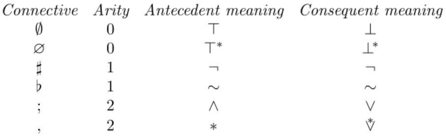
Figure 1 gives a summary of the structural connectives of our display calculus and their semantic reading as antecedents (or premises) and consequents (or conclusions) in a consecution. However, the presence of the meta-level negations ♯ and ♭ in our structures leads to a subtler notion of antecedent and consequent parts of consecutions than the simple left-right division of sequent calculus. Informally, moving inside a meta-level negation flips the interpretation of its immediate substructure. For example, if♯X or♭X is an antecedent part then the substructure X should be interpreted as a consequent part, and vice versa. This notion is made formal by the following definition.
Connective Arity Antecedent meaning Consequent meaning ∅ 0 ⊤ ⊥ ∅ 0 ⊤∗ ⊥∗ ♯ 1 ¬ ¬ ♭ 1 ∼ ∼ ; 2 ∧ ∨ , 2 ∗ ∨∗
Figure 1: The structural connectives of DLCBI.
Definition 3.2 (Antecedent part / consequent part). A structure occurrenceW is said to be apart of another structureZ if W occurs as a substructure of Z (in the obvious sense).
W is said to be a positive part of Z if W occurs inside an even number of occurrences of ♯
and ♭ inZ, and a negative part of Z otherwise.
A structure occurrenceW is said to be anantecedent part of a consecution X⊢Y if it is a positive part ofX or a negative part ofY. W is said to be aconsequent part ofX⊢Y
if it is a negative part ofX or a positive part ofY.
To give the formal interpretation of our consecutions in the following definition, we employ a pair of mutually recursive functions to capture the dependency between antecedent and consequent interpretations.
Definition 3.3 (Consecution validity). For any structure X we mutually define two for-mulas ΨX and ΥX by induction on the structure of X as follows:
ΨF = F ΥF = F Ψ∅ = ⊤ Υ∅ = ⊥ Ψ♯X = ¬ΥX Υ♯X = ¬ΨX ΨX1;X2 = ΨX1∧ΨX2 ΥX1;X2 = ΥX1∨ΥX2 Ψ∅ = ⊤∗ Υ∅ = ⊥∗ Ψ♭X = ∼ΥX Υ♭X = ∼ΨX ΨX1,X2 = ΨX1∗ΨX2 ΥX1,X2 = ΥX1 ∗ ∨ΥX2
A consecution X⊢Y is thenvalid if ΨX →ΥY is a valid formula (cf. Defn. 2.7).
We write a proof rule with a double line between premise and conclusion to indicate that it is bidirectional, i.e., that the roles of premise and conclusion may be reversed. A figure with three consecutions separated by two double lines is used to abbreviate two bidirectional rules in the obvious way.
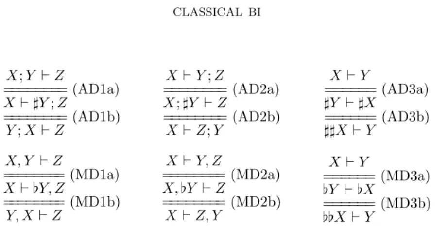
Definition 3.4 (Display-equivalence). Two consecutions X ⊢ Y and X′ ⊢Y′ are said to be display-equivalent, written X ⊢ Y ≡D X′ ⊢Y′, if there is a derivation of one from the
other using only the display postulates given in Figure 2.
The display postulates for DLCBI are essentially Belnap’s original display postulates, instantiated (twice) to the additive and multiplicative connective families of CBI. The only difference is that our postulates build commutativity of the comma and semicolon into the notion of display-equivalence, since in CBI both the conjunctions and both the disjunctions are commutative.
The fundamental characteristic of display calculi is their ability to “display” structures occurring in a consecution by rearranging it using the display postulates.
X;Y ⊢Z ======== (AD1a) X⊢♯Y;Z ======== (AD1b) Y;X ⊢Z X ⊢Y;Z ======== (AD2a) X;♯Y ⊢Z ======== (AD2b) X ⊢Z;Y X ⊢Y ====== (AD3a) ♯Y ⊢♯X ====== (AD3b) ♯♯X⊢Y X, Y ⊢Z ======== (MD1a) X⊢♭Y, Z ======== (MD1b) Y, X⊢Z X ⊢Y, Z ======== (MD2a) X, ♭Y ⊢Z ======== (MD2b) X ⊢Z, Y X⊢Y ====== (MD3a) ♭Y ⊢♭X ====== (MD3b) ♭♭X⊢Y
Figure 2: The display postulates for DLCBI.
Theorem 3.5(Display theorem (Belnap [2])). For any antecedent partW of a consecution
X⊢Y there exists a structureZ such thatW ⊢Z ≡D X⊢Y. Similarly, for any consequent
partW ofX ⊢Y there exists a structureZ such that Z ⊢W ≡D X ⊢Y.
Proof. Essentially, one uses the display postulates to move any structure surroundingW to the opposite side of the consecution, or to eliminate any preceding occurrences of ♯ and ♭
(note that for each possible position of W in X ⊢Y there are display postulates allowing the topmost level of structure above W to be moved away or eliminated). Moreover, each of the display postulates preserves antecedent and consequent parts of consecutions, so that
W must end up on the correct side of the consecution at the end of this process. The details are straightforward.
Example 3.6. The antecedent partY of the consecution♭(X, ♯Y)⊢Z;♭W can be displayed as follows: ♭(X, ♯Y)⊢Z;♭W (MD3a) ♭(Z;♭W)⊢♭♭(X, ♯Y) (MD3a,b) ♭♭♭(Z;♭W)⊢♭♭(X, ♯Y) (MD3a) ♭(X, ♯Y)⊢♭♭(Z;♭W) (MD3a) ♭(Z;♭W)⊢X, ♯Y (MD2b) ♭(Z;♭W), ♭X ⊢♯Y (AD3a) ♯♯Y ⊢♯(♭(Z;♭W), ♭X) (AD3a,b) Y ⊢♯(♭(Z;♭W), ♭X)
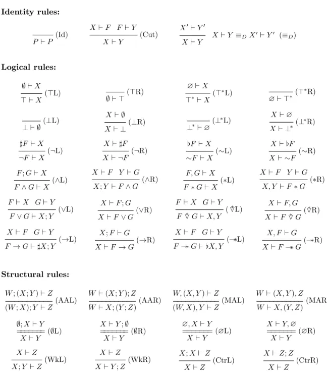
The proof rules of DLCBI are given in Figure 3. The identity rules consist of the usual identity axiom for propositional variables, a cut rule and a rule for display equivalence. The logical rules follow the division between left and right introduction rules familiar from sequent calculus. Note that, since we can appeal to Theorem 3.5, the formula introduced by a logical rule is always displayed in its conclusion. Both the identity rules and the logical rules are the standard ones for display logic, instantiated to CBI. The structural rules of DLCBIimplement suitable associativity and unitary laws on both sides of consecutions, plus weakening and contraction for the (additive) semicolon.
Identity rules: (Id) P ⊢P X ⊢F F ⊢Y (Cut) X ⊢Y X′⊢Y′ X ⊢Y ≡DX′ ⊢Y′ (≡ D) X ⊢Y Logical rules: ∅ ⊢X (⊤L) ⊤ ⊢X (⊤R) ∅ ⊢ ⊤ ∅⊢X (⊤∗L) ⊤∗⊢X (⊤∗R) ∅⊢ ⊤∗ (⊥L) ⊥ ⊢ ∅ X ⊢ ∅ (⊥R) X ⊢ ⊥ (⊥∗L) ⊥∗⊢∅ X⊢∅ (⊥∗R) X ⊢ ⊥∗ ♯F ⊢X (¬L) ¬F⊢X X ⊢♯F (¬R) X ⊢ ¬F ♭F ⊢X (∼L) ∼F ⊢X X ⊢♭F (∼R) X ⊢ ∼F F;G⊢X (∧L) F∧G⊢X X⊢F Y ⊢G (∧R) X;Y ⊢F∧G F, G⊢X (∗L) F∗G⊢X X ⊢F Y ⊢G (∗R) X, Y ⊢F∗G F⊢X G⊢Y (∨L) F∨G⊢X;Y X⊢F;G (∨R) X⊢F∨G F ⊢X G⊢Y (∨∗L) F ∨∗ G⊢X, Y X⊢F, G (∨∗R) X ⊢F ∨∗ G X ⊢F G⊢Y (→L) F→G⊢♯X;Y X;F⊢G (→R) X ⊢F →G X⊢F G⊢Y (—∗L) F —∗G⊢♭X, Y X, F ⊢G (—∗R) X ⊢F —∗G Structural rules: W; (X;Y)⊢Z =========== (AAL) (W;X);Y ⊢Z W ⊢(X;Y);Z =========== (AAR) W ⊢X; (Y;Z) W,(X, Y)⊢Z =========== (MAL) (W, X), Y ⊢Z W ⊢(X, Y), Z =========== (MAR) W ⊢X,(Y, Z) ∅;X⊢Y ======= (∅L) X ⊢Y X⊢Y;∅ ======= (∅R) X ⊢Y ∅, X⊢Y ======= (∅L) X ⊢Y X⊢Y,∅ ======= (∅R) X ⊢Y X ⊢Z (WkL) X;Y ⊢Z X ⊢Z (WkR) X ⊢Y;Z X;X ⊢Z (CtrL) X ⊢Z X ⊢Z;Z (CtrR) X ⊢Z
Figure 3: The proof rules of DLCBI. W, X, Y, Z range over structures,F, Grange over CBI-formulas andP ranges over V.
The identity axiom of DLCBIis postulated only for propositional variables5, but can be recovered for arbitrary formulas. We say a consecution iscut-free provable if it has a DLCBI proof containing no instances of (Cut).
Proposition 3.7. F ⊢F is cut-free provable in DLCBI for any formulaF. Proof. By structural induction onF.
Theorem 3.8 (Cut-elimination). If a consecution X ⊢ Y is provable in DLCBI then it is also cut-free provable.
Proof. The DLCBI proof rules satisfy the conditions shown by Belnap in [2] to be sufficient for cut-elimination to hold. We state these conditions and indicate how they are verified in Appendix A.
The following corollary of Theorem 3.8 uses the notion of asubformulaof a CBI-formula, defined in the usual way.
Corollary 3.9 (Subformula property). IfX ⊢Y is DLCBI-provable then there is a DLCBI proof of X ⊢Y in which every formula occurrence is a subformula of a formula occurring inX ⊢Y.
Proof. IfX ⊢Y is provable then it has a cut-free proof by Theorem 3.8. By inspection of the DLCBI rules, no rule instance in this proof can have in its premises any formula that is not a subformula of a formula occurring in its conclusion. Thus a cut-free proof of X ⊢Y
cannot contain any formulas which are not subformulas of formulas inX ⊢Y.
Corollary 3.10 (Consistency). Neither ∅⊢∅nor∅ ⊢ ∅is provable in DLCBI.
Proof. If ∅ ⊢ ∅ were DLCBI-provable then, by the subformula property (Corollary 3.9)
there is a proof of∅⊢∅containing no formula occurrences anywhere. But every axiom of
DLCBIcontains a formula occurrence, so this is impossible. Then ∅ ⊢ ∅cannot be provable either, otherwise ∅;∅⊢∅;∅ is provable by applying (WkL) and (WkR), whence ∅⊢∅ is
provable by applying (∅L) and (∅R), which is a contradiction. Our main technical results concerning DLCBI are the following.
Proposition 3.11 (Soundness). IfX⊢Y is DLCBI-provable then it is valid.
Proof. It suffices to show that each proof rule of DLCBI is locally sound in that validity of the conclusion follows from the validity of the premises. In the particular case of the display rule (≡D), local soundness follows by establishing that each display postulate (see Figure 2)
is locally sound. We show how to deal with some sample rule cases.
Case (—∗L).LetM =hR,◦, e,−,∞ibe a CBI-model, let r ∈R and suppose r |=ρF —∗G,
whence we require to show r |=ρ ∼ΨX ∨∗ ΥY. Using Lemma 2.8, it suffices to show that
r |=ρ ΨX —∗ ΥY. So, let r′, r′′ ∈ R be such that r′′ ∈ r ◦r′ and r′ |=ρ ΨX, whence we
require to showr′′|=ρΥY. Since the premiseX ⊢F is valid and r′|=ρΨX by assumption,
we haver′ |=ρF. Then, since r|=ρF —∗Gand r′′ ∈r◦r′, we haver′′|=ρG. Finally, since
the premiseG⊢Y is valid by assumption, we haver′′ |=ρΥY as required.
Case (∨L).∗ Let M =hR,◦, e,−,∞i be a CBI-model, let r ∈R and supposer |=ρF ∨∗ G,
whence we require to show r |=ρ ΥX ∨∗ ΥY. So, let r1, r2 ∈ R be such that −r ∈ r1 ◦r2, whence we require to show either −r1 |=ρ ΥX or −r2 |=ρ ΥY. Since −r ∈ r1 ◦r2 and
r |=ρ F ∨∗ G, we have either r1 |=ρ F or r2 |=ρ G. Then, since the premises F ⊢ X and
(Proposition 3.7) · · · F ⊢F (≡D) ♯F ⊢♯F (¬R) ♯F ⊢ ¬F (≡D) ♭¬F ⊢♭♯F (∼L) ∼¬F ⊢♭♯F (WkL) ∼¬F;∼F ⊢♭♯F (≡D) ♭F ⊢♭♯♭(∼¬F;∼F) (∼L) ∼F ⊢♭♯♭(∼¬F;∼F) (WkL) ∼¬F;∼F ⊢♭♯♭(∼¬F;∼F) (≡D) ♯♭(∼¬F;∼F)⊢♭(∼¬F;∼F) (WkL) ♭∅;♯♭(∼¬F;∼F)⊢♭(∼¬F;∼F) (≡D) ♭∅ ⊢♭(∼¬F;∼F);♭(∼¬F;∼F) (CtrR) ♭∅ ⊢♭(∼¬F;∼F) (≡D) ∼¬F ⊢♯∼F;∅ (∅R) ∼¬F ⊢♯∼F (¬R) ∼¬F ⊢ ¬∼F
Figure 4: A cut-free DLCBI proof of∼¬F ⊢ ¬∼F.
Case (MAR).Both directions of the rule follow by establishing that for any CBI-model
M =hR,◦, e,−,∞i and r ∈R we have r |=ρΥX ∨∗ (ΥY ∨∗ ΥZ) iff r |=ρ (ΥX ∨∗ ΥY) ∨∗ ΥZ.
Using the equivalences F ∨∗ G ↔ ∼(∼F ∗ ∼G) and ∼∼F ↔ F given by Lemma 2.8, it suffices to show thatr |=ρ∼(∼ΥX∗(∼ΥY ∗ ∼ΥZ)) iff r|=ρ∼((∼ΥX∗ ∼ΥY)∗ ∼ΥZ). This
follows straightforwardly from the definition of satisfaction and the associativity of ◦. Case (MD1a).We show how to treat one direction of this display postulate; the reverse direction is symmetric. Let M = hR,◦, e,−,∞i be a CBI-model, let r ∈ R and suppose that r |=ρΨX, whence we require to show r|=ρ∼ΨY ∨∗ ΥZ. By Lemma 2.8, it suffices to
show r |=ρ ΨY —∗ ΥZ. So let r′, r′′ ∈ R be such that r′′ ∈ r ◦r′ and r′ |=ρ ΨY, whence
we require to show r′′ |=
ρ ΥZ. Sincer |=ρ ΨX we have r′′ |=ρ ΨX ∗ΨY, whence we have
r′′|=ρΥZ as required because the premiseX, Y ⊢Z is assumed valid.
Theorem 3.12 (Completeness of DLCBI). IfX ⊢Y is valid then it is provable in DLCBI. We give the proof of Theorem 3.12 in Section 4.
We remark that, although cut-free proofs in DLCBIenjoy the subformula property, they do not enjoy the analogous “substructure property”, and cut-free proof search in our system is still highly non-deterministic due to the presence of the display postulates and structural rules, the usage of which cannot be straightforwardly constrained in general. In Figure 4 we
give a sample cut-free proof of the consecution∼¬F ⊢ ¬∼F, which illustrates the problems. The applications of display-equivalence are required in order to apply the logical rules, as one would expect, but our derivation also makes essential use of contraction, weakening and a unitary law. It is plausible that the explicit use of at least some of these structural rules can be eliminated by suitable reformulations of the logical rules. However, the inherent nondeterminism in proof search cannot be removed by refining DLCBI without loss of power since, by soundness and completeness, provability in DLCBIis equivalent to validity in CBI, which has been recently shownundecidable by the first author and Kanovich [7]. This is not fundamentally surprising, since at least some displayable logics are known to be undecidable; indeed, one of Belnap’s original applications of display logic was in giving a display calculus for the full relevant logic R, which was famously proven undecidable by Urquhart [48]. (Unfortunately, we cannot distinguish decidable display calculi from undecidable ones in general; the decidability of an arbitrary displayable logic was itself shown undecidable by Kracht [29].)
Nonetheless, we argue that there are good reasons to prefer our DLCBI over arbitrary complete proof systems (e.g. Hilbert systems) without cut-elimination. Display calculi in-herit the main virtues of traditional Gentzen systems: they distinguish structural princi-ples from logical ones, and make explicit the considerable proof burden that exists at the meta-level, but nevertheless retain a theoretically very elegant and symmetric presentation. Furthermore, as a result of the subformula property one has in display calculi what might be called a property of “finite choice” for proof search: for any consecution there are only finitely many ways of applying any rule to it in a backwards fashion6.
4. Completeness of DLCBI
In this section we prove completeness of our display calculus DLCBI with respect to validity in CBI-models. As in the case of the analogous result for BBI in [10], our result hinges on a general completeness theorem for modal logic due to Sahlqvist. However, we also require an extra layer of translation between Hilbert-style proofs and proofs in DLCBI. Our proof is divided into three main parts. First, in subsection 4.1, we reinvent CBI as a modal logic by defining a class of standard modal frames, with associated modalities corresponding to the standard CBI-model operations, that satisfy a certain set of modal logic axioms. By appealing to Sahlqvist’s completeness theorem, we obtain a complete Hilbert-style proof theory for this class of frames. It then remains to connect the modal presentation of CBI to our standard presentation. In subsection 4.2, we show that the aforementioned class of modal frames is exactly the class of CBI-models given by Definition 2.2. Then, in subsection 4.3, we show how to translate any modal logic proof into a DLCBI proof. Thus we obtain the DLCBI-provability of any valid consecution.
4.1. CBI as a modal logic. In this subsection we define the semantics of a modal logic corresponding to CBI, and obtain a complete proof theory with respect to this semantics, all using standard modal techniques (see e.g. [4]).
We first define MLCBIframes, which are standard modal frames with associated modal-ities corresponding to the CBI-model operations in Definition 2.2.
6In fact, this is not quite true as it stands because for any consecution there are infinitely many consecu-tions that are display-equivalent to it, obtained by “stacking” occurrences of♯and♭. However, by identifying structures such as♯♯XandX, one obtains only finitely many display-equivalent consecutions. See e.g. [43].
Definition 4.1.1 (Modal logic frames). An MLCBI frame is a tuple hR,◦,−•, e,−,∞i, where ◦:R×R→ P(R), −•:P(R)× P(R)→ P(R), e⊆R,−:R→ P(R), and ∞ ⊆ R. We extend ◦ to P(R)× P(R) → P(R), and − to P(R) → P(R), in the same pointwise manner as in Definition 2.2. If eis a singleton set then the frame is said to beunitary.
Definition 4.1.2 (Modal logic formulas). Modal logic formulas A are defined by:
A::=P | ⊤ | ⊥ | ¬A|A∧A|A∨A|A→A|e| ∞ | −A|A◦A|A−•A
where P ranges over V. We remark that we read e,∞,−,◦,−• as modalities (with the obvious arities). We regard →as having weaker precedence than these modalities, and use parentheses to disambiguate where necessary.
The satisfaction relation for modal logic formulas in MLCBI frames is defined exactly as in Definition 2.6 for the additive connectives, and the modalities are given a “diamond” possibility interpretation: r|=ρe ⇔ r∈e r |=ρ∞ ⇔ r∈ ∞ r|=ρ−A ⇔ ∃r′∈R. r∈ −(r′) and r′|=ρA r |=ρA1◦A2 ⇔ ∃r1, r2∈R. r∈r1◦r2 and r1 |=ρA1 and r2 |=ρA2 r |=ρA1−•A2 ⇔ ∃r1, r2∈R. r∈r1−•r2 and r1 |=ρA1 and r2 |=ρA2
We remark that the −• modality — which does not correspond directly to a CBI-model operation but should be read informally as ¬(A1—∗ ¬A2) — will be helpful later in giving a modal axiomatisation of CBI-models; see Defn. 4.1.6. We could alternatively employ a modality corresponding directly to —∗, but it is much more technically convenient to work exclusively with “diamond” modalities.
Given any set Aof modal logic axioms, we defineA-models to be those MLCBI frames in which every axiom in Aholds. The standard modal logic proof theory corresponding to the class ofA-models is given by the following definition (cf. [4]).
Definition 4.1.3 (Modal logic proof theory). The modal logic proof theory generated by a setA of modal logic axioms, denoted by LA, consists of some fixed finite axiomatisation of propositional classical logic, extended with the following axioms and proof rules:
(A) : A for each A∈ A (−⊥) : −⊥ → ⊥ (◦⊥) : P ◦ ⊥ → ⊥ (−•⊥) : (⊥ −•P)∨(P −• ⊥)→ ⊥ (−∨) : −(P ∨Q)↔ −P∨ −Q (◦∨) : (P ∨Q)◦R↔(P◦R)∨(Q◦R) (−•∨L) : (P ∨Q)−•R↔(P−•R)∨(Q−•R) (−•∨R) : P −•(Q∨R)↔(P−•Q)∨(P−•R) A→B A (MP) B A (Subst) A[B/P] A→B (⋄−) (−A)→(−B) A→B (⋄◦) (A◦C)→(B◦C) A→B (⋄−•L) (C−•A)→(C−•B) A→B (⋄−•L) (A−•C)→(B−•C)
where A, B, C range over modal logic formulas, P, Q, R are propositional variables, and
A↔B is as usual an abbreviation for (A→B)∧(B →A).
Note that the axioms and rules for the modalities which are added to A by Defini-tion 4.1.3 are just the axioms and rules of the standard modal logic K, instantiated to each of our “diamond”-type modalitiese,∞,−,◦and−•. We emphasise that, by definition, the latter are diamond modalities rather than logical connectives. In particular, the modality ‘−’ is not a negation (−Ashould be understood informally as the CBI-formula∼¬A), and is monotonic rather than antitonic with respect to entailment, as embodied by the rule (⋄−). Similarly, the −• modality is monotonic in its left-hand argument because it is a diamond modality and not an implication.
We now state a sufficient condition, due to Sahlqvist, for completeness of LA to hold with respect to the class of A-models.
Definition 4.1.4 (Very simple Sahlqvist formulas). A very simple Sahlqvist antecedent S
is a formula given by the grammar:
S ::=⊤ | ⊥ |P |S∧S |e| ∞ | −S|S◦S|S−•S
whereP ranges overV. Avery simple Sahlqvist formula is a modal logic formula of the form
S → A+, whereS is a very simple Sahlqvist antecedent and A+ is a modal logic formula which is positive in that no propositional variable P in A+ may occur inside the scope of an odd number of occurrences of ¬.
Theorem 4.1.5 (Sahlqvist [4]). Let A be a set of modal logic axioms consisting only of very simple Sahlqvist formulas. Then the modal logic proof theory LA is complete with respect to the class of A-models. That is, if a modal logic formula F is valid with respect to A-models then it is provable in LA.
Definition 4.1.6 (Modal logic axioms for CBI). The axiom set AXCBI consists of the following modal logic formulas, whereP, Q, R are propositional variables:
(1) e◦P → P (2) P →e◦P (3) P ◦Q→Q◦P (4) (P ◦Q)◦R →P ◦(Q◦R) (5) P ◦(Q◦R)→(P◦Q)◦R (6) Q∧(R◦P)→(R∧(P−•Q))◦ ⊤ (7) R∧(P−•Q)→(⊤−•(Q∧(R◦P))) (8) −−P →P (9) P → −−P (10) −P →(P −• ∞) (11) (P−• ∞)→ −P
By inspection we can observe that the AXCBI axioms (cf. Definition 4.1.6) are all very simple Sahlqvist formulas, whence we obtain from Theorem 4.1.5:
Corollary 4.1.7. If a modal logic formula F is valid with respect to AXCBI-models then it is provable in LAXCBI.
We show that the completeness result transfers to unitary AXCBI-models.
Lemma 4.1.8. Let M =hR,◦,−•, e,−,∞i be an AXCBI model. Then there exist unitary AXCBI-models Mx for each x∈esuch that the following hold:
(1) M is the disjoint union of the modelsMx forx∈e.
Proof. For each x ∈ e, the model Mx is defined by restricting M to Rx =def {r ∈ R | {r} ◦ {x} 6= ∅}. Disjointness of models follows directly from the fact that hR,◦, ei obeys the first five axioms of AXCBI, which characterize relational commutative monoids. Finally, (1)⇒(2) is a general result which holds in modal logic [4].
Corollary 4.1.9. If a modal logic formulaF is valid with respect tounitary AXCBI-models then it is provable in LAXCBI.
4.2. CBI-models as modal logic models.
Lemma 4.2.1. IfhR,◦, e,−,∞iis a CBI-model then, for all X, Y, Z ∈ P(R), we have: (1) X◦Y =Y ◦X and X◦(Y ◦Z) = (X◦Y)◦Z and {e} ◦X=X
(2) −X =X−• ∞ (3) −−X=X
whereX−•Y =def {z∈R | ∃x∈X, y∈Y. y∈x◦z}.
Proof. The required properties follow straightforwardly from the properties of CBI-models given by Definition 2.2 and Proposition 2.3.
Lemma 4.2.2. Let hR,◦,−•, e,−,∞i be an unitary AXCBI-model (so that e is a single-ton set). Then ∞ is a singleton set, and −x is a singleton set for any x ∈ R. Moreover, hR,◦, e,−,∞iis a CBI-model with the modalities e,−,∞regarded as having the appropri-ate types.
Proof. We first show that −x is a singleton by contradiction, using the fact that −−x = {x} must hold for any set x, as a consequence of axioms (8) and (9). If −x = ∅ then −−x = S
y∈−x−y =∅, which contradicts −−x = {x}. If x1, x2 ∈ −x with x1 6=x2, then −x1∪ −x2 ⊆ − −x. Also,−x1 6=−x2, otherwise we would have {x1} =−−x1 =−−x2 = {x2} and thus x1 = x2. Since −x1 and −x2 have cardinality > 0 (see above), −−x must have cardinality >1, which contradicts −−x={x}.
We prove that ∞ is a singleton by deriving ∞ = −e. Using the axioms in Defini-tion 4.1.6, we will show thate−•X =X must hold for any setX. This fact, together with axioms (10) and (11) instantiated with P =e gives the desired consequence∞=−e.
It remains to showe−•X =X. Axioms (6) and (7) give the two directions of:
q ∈r◦p iff r∈p−•q
for any p, q, r∈R, and axioms (1), (2) and (3) give, for anyx∈R:
x◦e={x} Therefore we have that, for any x∈R:
Definition 4.2.3 (Embedding of CBI-models in AXCBI-models). Let M =hR,◦, e,−,∞i be a CBI-model. The tuple pMq = hR,◦,−•, e,−,∞i is obtained by regarding e,−,∞ as
having the same types as in Definition 4.1.1 in the obvious way, and by defining the modality −•:P(R)× P(R)→ P(R) byX−•Y =def {z∈R | ∃x∈X, y∈Y. y∈x◦z}.
Lemma 4.2.4. IfM is a CBI-model then pMq is a unitary AXCBI-model. Moreover, the
functionp−q is a bijection between CBI-models and unitary AXCBI-models.
Proof. First observe that in any MLCBI frame hR,◦,−•, e,−,∞i, the AXCBI axioms (6) and (7) hold iff we have, for allX, Y inP(R):
X−•Y ={z∈R| ∃x∈X, y ∈Y. y∈x◦z}
LetMbe a CBI-model. Then axioms (6) and (7) hold inpMqby the above observation. The
remaining AXCBI axioms hold in pMq as a direct consequence of Lemma 4.2.1. Therefore pMqis a unitary AXCBI-model.
It remains to show that p−q is a bijection. Injectivity is immediate by definition. For
surjectivity, letM′ =hR,◦,−•, e,−,∞ibe a unitary AXCBImodel. By Lemma 4.2.2 we have thathR,◦, e,−,∞iis a CBI-model. Since the interpretation of−•is determined by◦because of the above observation about axioms (6) and (7), it follows that phR,◦, e,−,∞iq =M′,
hence p−q is surjective.
Definition 4.2.5 (Translation of CBI-formulas to modal logic formulas). We define a func-tionp−qfrom formulas to modal logic formulas by induction on the structure of
CBI-formulas, as follows: pFq = F whereF ∈ {P,⊤,⊥} p⊤∗q = e pF1?F2q = pF1q?pF2q where ?∈ {∧,∨,→} pF1 ∗ F2q = pF1q ◦ pF2q pF1 —∗ F2q = ¬(pF1q −• ¬pF2q) p¬Fq = ¬pFq p⊥∗q = ¬∞ p∼Fq = ¬−pFq pF1 ∨∗ F2q = ¬−(¬−pF1q◦ ¬−pF2q)
where P in the first clause ranges over V. We extend the domain of p−q to DLCBI
conse-cutions by:
pX ⊢Yq=pΨXq→pΥYq
where Ψ− and Υ− are the functions given in Definition 3.3.
In the following, we write F[G/P] to denote the result of substituting the formula G
for all occurrences of the propositional variable P in the formulaF. This notation applies both to CBI-formulas and to modal logic formulas.
Lemma 4.2.6. LetF be a CBI-formula, andM =hR,◦, e,−,∞ia CBI-model. ThenF is true in M if and only if pFq is true inpMq.
Proof. LetF be a CBI-formula and A a modal logic formula. We defineF ≃A to hold iff for all environmentsρ, and allr ∈R, the following holds:
r|=ρF wrt.M ⇔ r |=ρA wrt.pMq
(1) F ≃A and G≃B implies F[G/P]≃A[B/P] (2) ⊤∗ ≃e (3) P1∗P2 ≃P1◦P2 (4) P1 —∗P2 ≃ ¬(P1 −• ¬P2) (5) ⊥∗ ≃ ¬∞ (6) ∼P ≃ ¬−P (7) P1 ∨∗ P2≃ ¬−(¬−P1◦ ¬−P2)
We show one interesting case (7). By Lemma 2.8 we have that P1 ∨∗ P2 is equivalent to ∼(∼P1∗ ∼P2), therefore it is sufficient to prove ∼(∼P1 ∗ ∼P2) ≃ ¬−(¬−P1◦ ¬−P2). By (6) we have ∼Pi ≃ ¬−Pi for i ∈ {1,2}, hence by (1) and (3) we obtain (∼P1 ∗ ∼P2) ≃ (¬−P1◦ ¬−P2). Thus by (1) and (6) we conclude∼(∼P1∗ ∼P2)≃ ¬−(¬−P1◦ ¬−P2), as required.
The second part establishes F ≃ pFq by induction on the structure of F, using the
results from the first part.
Proposition 4.2.7. A consecution X ⊢ Y is valid (wrt. CBI-models) iff pΨX →ΥYq is
valid wrt. unitary AXCBI-models.
Proof. By definition, X ⊢ Y is valid iff ΨX → ΥY is true in every CBI-model M. By
Lemma 4.2.6, this is equivalent to:
pΨX →ΥYqis true in pMq for every CBI-model M
Since p−qis a bijection onto unitary AXCBI-models by Lemma 4.2.4, this is equivalent to: pΨX →ΥYq is true in all unitary AXCBI-models
i.e. pΨX →ΥYq is valid wrt. unitary AXCBI-models.
By combining Proposition 4.2.7 and Corollary 4.1.9 we obtain the following key inter-mediate result towards completeness for DLCBI:
Corollary 4.2.8. IfX ⊢Y is a valid consecution thenpΨX →ΥYqis provable in LAXCBI.
4.3. From modal logic proofs to DLCBI proofs.
Definition 4.3.1 (Translation from modal logic formulas to CBI-formulas). We define a function x−y from modal logic formulas to CBI-formulas by induction on the structure of
CBI-formulas, as follows: xAy = A where A∈ {P,⊤,⊥} x¬Ay = ¬xAy xA1?A2y = xA1y?xA2y where ?∈ {∧,∨,→} xA1◦A2y = xA1y ∗ xA2y xA1 −• A2y = ¬(xA1y—∗ ¬xA2y) xey = ⊤∗ x−Ay = ¬∼xAy x∞y = ¬⊥∗
Proposition 4.3.2. The axioms and proof rules of LAXCBI(cf. Defn. 4.1.3) are admissible in DLCBI under the embeddingA7→(∅ ⊢xAy) from modal logic formulas to consecutions.
(Prop. 3.7) · · · R⊢R (Prop. 3.7) · · · P⊢P (Prop. 3.7) · · · Q⊢Q (≡D) ♯Q⊢♯Q (¬L) ¬Q⊢♯Q (WkR) ¬Q⊢♯Q; (R∧ ¬(P —∗ ¬Q))∗ ⊤ (—∗L) P —∗ ¬Q⊢♭P,(♯Q; (R∧ ¬(P —∗ ¬Q))∗ ⊤) (≡D) ♯(♭P,(♯Q; (R∧ ¬(P —∗ ¬Q))∗ ⊤))⊢♯P —∗ ¬Q (¬R) ♯(♭P,(♯Q; (R∧ ¬(P —∗ ¬Q))∗ ⊤))⊢ ¬(P —∗ ¬Q) (∧R) R;♯(♭P,(♯Q; (R∧ ¬(P —∗ ¬Q))∗ ⊤))⊢R∧ ¬(P —∗ ¬Q) (⊤R) ∅ ⊢ ⊤ (WkR) ∅;P ⊢ ⊤ (∅R) P ⊢ ⊤ (∗R) (R;♯(♭P,(♯Q; (R∧ ¬(P —∗ ¬Q))∗ ⊤))), P ⊢(R∧ ¬(P —∗ ¬Q))∗ ⊤ (WkR) (R;♯(♭P,(♯Q; (R∧ ¬(P —∗ ¬Q))∗ ⊤))), P ⊢♯Q; (R∧ ¬(P —∗ ¬Q))∗ ⊤ (≡D) R⊢(♭P,(♯Q; (R∧ ¬(P —∗ ¬Q))∗ ⊤)); (♭P,(♯Q; (R∧ ¬(P —∗ ¬Q))∗ ⊤)) (CtrR) R⊢♭P,(♯Q; (R∧ ¬(P —∗ ¬Q))∗ ⊤) (≡D) R, P ⊢♯Q; (R∧ ¬(P —∗ ¬Q))∗ ⊤ (∗L) R∗P⊢♯Q; (R∧ ¬(P—∗ ¬Q))∗ ⊤ (≡D) Q;R∗P ⊢(R∧ ¬(P—∗ ¬Q))∗ ⊤ (∧L) Q∧(R∗P)⊢(R∧ ¬(P —∗ ¬Q))∗ ⊤ (∅L) ∅;Q∧(R∗P)⊢(R∧ ¬(P —∗ ¬Q))∗ ⊤ (→R) ∅ ⊢Q∧(R∗P)→(R∧ ¬(P —∗ ¬Q))∗ ⊤
Figure 5: A DLCBIderivation of the LAXCBIaxiom (6) under the embeddingA7→(∅ ⊢xAy),
needed for the proof of Proposition 4.3.2.
Proof. First, we note that all of the proof rules of LAXCBI, except (Subst), are easily derivable in DLCBI under the embedding. The rule (Subst) is admissible in DLCBI (under the embedding) because each of its proof rules is closed under the substitution of arbitrary formulas for propositional variables; in the case of the axiom rule (Id) this requires an appeal to Proposition 3.7.
It remains to show that ∅ ⊢xAy is DLCBI-derivable for every axiomA of LAXCBI. The AXCBI axioms are mainly straightforward, with the chief exceptions being axioms (6) and (7). (We remark that axioms (8) and (9) are straightforward once one has DLCBI proofs that ¬ and ∼ commute; see Figure 4 for a proof of ∼¬F ⊢ ¬∼F.) In the case of AXCBI axiom (6), we need to show the consecution ∅ ⊢ Q∧(R∗P) → (R∧ ¬(P —∗ ¬Q))∗ ⊤ is provable in DLCBI. We give a suitable derivation in Figure 5. The treatment of AXCBI axiom (7) is broadly similar. It remains to treat the generic modal logic axioms of LAXCBI, which again are mainly straightforward and involve showing distribution of the modalities over ∨. E.g., in the case of the axiom (−•∨L) we require to show that ∅ ⊢ ¬((P ∨Q) —∗
(Id) P ⊢P (Id) R⊢R (≡D) ♯R⊢♯R (¬L) ¬R⊢♯R (—∗L) P —∗ ¬R⊢♭P, ♯R (WkL) P —∗ ¬R;Q—∗ ¬R⊢♭P, ♯R (≡D) P ⊢♯R, ♭(P —∗ ¬R;Q—∗ ¬R) (Id) Q⊢Q (Id) R⊢R (≡D) ♯R⊢♯R (¬L) ¬R⊢♯R (—∗L) Q—∗ ¬R⊢♭Q, ♯R (WkL) P —∗ ¬R;Q—∗ ¬R⊢♭Q, ♯R (≡D) Q⊢♯R, ♭(P —∗ ¬R;Q—∗ ¬R) (∨L) P∨Q⊢(♯R, ♭(P —∗ ¬R;Q—∗ ¬R)); (♯R, ♭(P —∗ ¬R;Q—∗ ¬R)) (CtrR) P∨Q⊢♯R, ♭(P —∗ ¬R;Q—∗ ¬R) (≡D) (P —∗ ¬R;Q—∗ ¬R), P ∨Q⊢♯R (¬R) (P —∗ ¬R;Q—∗ ¬R), P ∨Q⊢ ¬R (—∗R) P —∗ ¬R;Q—∗ ¬R⊢(P ∨Q) —∗ ¬R (≡D) ♯(P∨Q) —∗ ¬R;Q—∗ ¬R⊢♯P —∗ ¬R (¬R) ♯(P∨Q) —∗ ¬R;Q—∗ ¬R⊢ ¬(P —∗ ¬R) (≡D) ♯(P∨Q) —∗ ¬R;♯¬(P —∗ ¬R)⊢♯Q—∗ ¬R (¬R) ♯(P∨Q) —∗ ¬R;♯¬(P —∗ ¬R)⊢ ¬(Q—∗ ¬R) (≡D) ♯(P∨Q) —∗ ¬R⊢ ¬(P —∗ ¬R);¬(Q—∗ ¬R) (¬L) ¬((P∨Q) —∗ ¬R)⊢ ¬(P —∗ ¬R);¬(Q—∗ ¬R) (∨R) ¬((P∨Q) —∗ ¬R)⊢ ¬(P —∗ ¬R)∨ ¬(Q—∗ ¬R) (∅L) ∅;¬((P∨Q) —∗ ¬R)⊢ ¬(P —∗ ¬R)∨ ¬(Q—∗ ¬R) (→R) ∅ ⊢ ¬((P ∨Q) —∗ ¬R)→ ¬(P —∗ ¬R)∨ ¬(Q—∗ ¬R)
Figure 6: A DLCBI derivation of (one direction of) the LAXCBI axiom (−•∨L) under the embedding A7→(∅ ⊢xAy), needed for the proof of Proposition 4.3.2.
¬R)↔ ¬(P —∗ ¬R)∨ ¬(Q—∗ ¬R) is DLCBI-derivable. We give a derivation of one direction of this bi-implication in Figure 6. The other direction of the bi-implication, and the other axioms, are derived in a similar fashion.
The following corollary of Proposition 4.3.2 is immediate by induction over the structure of LAXCBI proofs.
Corollary 4.3.3. If Ais provable in LAXCBI then ∅ ⊢xAy is provable in DLCBI.
We write F ⊣⊢ G, where F and G are CBI-formulas, to mean that both F ⊢ G and
G ⊢F are provable (in DLCBI), and call F ⊣⊢ G a derivable equivalence (of DLCBI). We observe that derivable equivalence in DLCBI is indeed an equivalence relation: it is reflexive by Proposition 3.7, symmetric by definition and transitive by the DLCBI rule (Cut).
(I.H.) · · · F1⊢xpF1qy (≡D) ♭xpF1qy⊢♭F1 (∼L) ∼xpF1qy⊢♭F1 (≡D) ♯♭F1⊢♯∼xpF1qy (¬R) ♯♭F1⊢ ¬∼xpF1qy (≡D) ♯¬∼xpF1qy⊢♭F1 (¬L) ¬¬∼xpF1qy⊢♭F1 (≡D) F1⊢♭¬¬∼xpF1qy (I.H.) · · · F2⊢xpF2qy (≡D) ♭xpF2qy⊢♭F2 (∼L) ∼xpF2qy⊢♭F2 (≡D) ♯♭F2⊢♯∼xpF2qy (¬R) ♯♭F2⊢ ¬∼xpF2qy (≡D) ♯¬∼xpF2qy⊢♭F2 (¬L) ¬¬∼xpF2qy⊢♭F2 (≡D) F2⊢♭¬¬∼xpF2qy (∨∗L) F1∨∗ F2⊢♭¬¬∼xpF1qy, ♭¬¬∼xpF2qy (≡D) ¬¬∼xpF1qy,¬¬∼xpF2qy⊢♭F1∨∗ F2 (∗L) ¬¬∼xpF1qy∗ ¬¬∼xpF2qy⊢♭F1∨∗ F2 (≡D) F1∨∗ F2⊢♭¬¬∼xpF1qy∗ ¬¬∼xpF2qy (∼R) F1∨∗ F2⊢ ∼(¬¬∼xpF1qy∗ ¬¬∼xpF2qy) (≡D) ♯∼(¬¬∼xpF1qy∗ ¬¬∼xpF2qy)⊢♯F1∨∗ F2 (¬L) ¬∼(¬¬∼xpF1qy∗ ¬¬∼xpF2qy)⊢♯F1∨∗ F2 (≡D) F1∨∗ F2⊢♯¬∼(¬¬∼xpF1qy∗ ¬¬∼xpF2qy) (¬R) F1∨∗ F2⊢ ¬¬∼(¬¬∼xpF1qy∗ ¬¬∼xpF2qy)
Figure 7: A DLCBI proof for the non-trivial case of Lemma 4.3.4.
Proof. By combining the definitions ofp−q and x−y (cf. Defns. 4.2.5 and 4.3.1) we obtain
the following definition of xp−qy, given by structural induction on CBI-formulas: xpFqy = F whereF ∈ {P,⊤,⊥,⊤∗} xp¬Fqy = ¬xpFqy xpF1 ?F2qy = xpF1qy?xpF2qy where ?∈ {∧,∨,→,∗} xp⊥∗qy = ¬¬⊥∗ xp∼Fqy = ¬¬∼xpFqy xpF1 —∗F2qy = ¬¬(xpF1qy—∗ ¬¬xpF2qy) xpF1 ∗ ∨F2qy = ¬¬∼(¬¬∼xpF1qy∗ ¬¬∼xpF2qy)
With this in mind, we now proceed by structural induction on F. The base cases, in which xpFqy = F, are immediate since F ⊣⊢ F is a derivable equivalence of DLCBI by
Proposition 3.7. Most of the other cases are straightforward using the induction hypothesis and the fact that¬¬F ⊣⊢F is easily seen to be a derivable equivalence of DLCBI. We show one direction of the only non-trivial case, F =F1 ∨∗ F2, in Figure 7. The reverse direction is similar.
The following two lemmas, which show how to construct proofs of arbitrary valid con-secutions given proofs of arbitrary valid formulas, are standard in showing completeness of display calculi relative to Hilbert-style proof systems, and were first employed by Gor´e [24].
Lemma 4.3.5. For any structure X the consecutions X ⊢ ΨX and ΥX ⊢ X are both
DLCBI-provable.
Proof. By structural induction onX. The case whereXis a formulaF follows directly from Proposition 3.7. The other cases all follow straightforwardly from the induction hypothesis and the logical rules of DLCBI. E.g., whenX =♭Y we have ΨX =∼ΥY and ΥX =∼ΨY,
and proceed as follows:
(I.H.) · · · ΥY ⊢Y (≡D) ♭Y ⊢♭ΥY (∼R) ♭Y ⊢ ∼ΥY (I.H.) ·