Proof systems for Moss coalgebraic logic

Proof systems for Moss’ coalgebraic logic

January 7, 2013

Abstract

We study Gentzen-style proof theory of the finitary version of the coalgebraic logic in-troduced by L. Moss. The logic captures the behaviour of coalgebras for a large class of set functors. The syntax of the logic, defined uniformly with respect to a finitary coalgebraic type functor T, uses a single modal operator ∇T of arity given by the functor T itself,

and its semantics is defined in terms of a relation lifting functorT. An axiomatization of the logic, consisting of modal distributive laws, has been given together with an algebraic completeness proof in work of C. Kupke, A. Kurz and Y. Venema.

In this paper, following our previous work on structural proof theory of the logic in the special case of the finitary powerset functor, we present cut-free, one- and two-sided sequent calculi for the finitary version of Moss’ coalgebraic logic for a general finitary functor T in a uniform way. For the two-sided calculi to be cut-free we use a language extended with the boolean dual of the nabla modality.

Keywords: modal logic, coalgebraic logic, sequent system, coalgebra, cover modality, Gentzen calculus, completeness.

1

Introduction

The theory of coalgebras, introduced by Aczel in the late 1980s [1, 2], is a fast-growing research area in theoretical computer science which provides a unifying framework for state-based evolving systems. The unifying power of the coalgebraic theory of systems lies in that various classes of systems can be formalized as coalgebras of appropriate set (endo)functorsT

(representing thetypeof the given class); hence their theory can be developed parametrically in T. As a key example, any set functor T canonically induces a notion of observational or

behavioural equivalence between T-coalgebras; this notion generalizes the natural notions of bisimilarity which were independently developed for each specific type of system.

In order to describe and reason about the behaviour of systems modelled by coalgebras, specification languages and derivation systems have been introduced, which gave rise to a research programme in its own right, namely coalgebraic logic. Coherently with the spirit

∗

The research of the first author has been supported by grant P202/11/P304 of the Czech Grant Agency, and by the Programme for the Development of Fields of Study at Charles University, No. P13 Rationality in human sciences, subprogramme Modern logics, their methods and applications. The research of the second author has been made possible by the VENI grant 639.031.726 of the Netherlands Organization for Scientific Research (NWO). The research of the third author has been made possible by the NWO VICI grant 639.073.501.

of the coalgebraic theory of systems, coalgebraic logic aims at developing logical formalisms which can be defined and studied uniformly in the functor T. Since Kripke models and frames are exactly the P-coalgebras, i.e. the coalgebras of the powerset functor, and since

modal logic is the archetypal bisimulation-invariant logic, the several current proposals for suitable coalgebraic logics, such as based on the so-called predicate lifting modalities [19, 25], or equivalently modalities arising from Stone type dualities [7, 14], or a framework making use of co-equations [3], are set out as generalizations of modal logic in some respects.

In the above mentioned framework of coalgebraic logic based on predicate liftings an ex-tensive work has been done in the direction of proof theory and its applications by L. Schr¨oder and D. Pattinson. Namely, in [20] sequent systems have been defined systematically from a given axiomatization of a logic, and cut admissibility has been proven for strictly one-step complete logics; in [21, 22] one-step completeness has been related to eliminability of cuts and a purely syntactic condition on the modal part of a calculus has been given for the calculus to admit cut elimination.

The research line of the present paper was initiated by Moss [17]; he defined an elegant generalization of modal logic, using the functor T to define a modal connective ∇T which takes in input elements α ∈ TωL (where Tω is the finitary version of T, and L denotes the collection of formulas), and returns formulas∇_Tα.

IfT is the powerset functorP, its associated connective∇P takes a finiteset αof formulas and returns a single formula∇Pα. The semantics of∇P is defined as follows, for an arbitrary Kripke structureS with accessibility relationR:

S, s∇α if for all a∈α there is at∈R[s] with S, ta, and

for all t∈R[s] there is ana∈α withS, ta. (1)

The modal connective∇can be seen as a defined connective in the standard modal language:

∇α=2(_α)∧^3α, (2)

where3αdenotes the set{3a|a∈α}. But in fact the following semantic equivalences hold for∇interpreted as in (1):

3α ≡ ∇{α,>} 2α ≡ ∇∅∨ ∇{α}, (3)

which show that the language based on ∇ is an alternative formulation of standard modal logic.

Analogously to the duality between2 and 3,∇admits a dual operator ∆, which, inter-estingly, can be defined in the following, negation-free way:

∆α= ( ∇_∅∨W {∇{a} | a∈α} ∨ ∇{V α,>} ifα6=∅ ∇{>} ifα=∅ (4) The ∇-based reformulation of modal logic lends itself naturally to a coalgebraic general-ization, thanks to the following fundamental observation, due to Moss [17]: the satisfaction clause (1) is equivalent to

whereP() denotes the Egli-Milner (i.e. theP-)relation lifting of the satisfaction relation

between states and formulas. Hence, for every set-endofunctorT, everyT-coalgebraσ:X →

T X× P(AtP rop) and every state s∈X,

σ, s∇_Tα iff (σ(s), α)∈T(), (6)

whereT()⊆T X ×TL denotes theT-relation lifting of ⊆X× L(see also Definition 2.7 for more details and discussion). A well-behaved functorial relation lifting is not available in general: it is available for a large class of set functors, namely for those preserving weak pullbacks. (For the same class of functors bisimilarity captures behavioural equivalence.) It leaves out certain interesting functors, for example the double contravariant powerset functor

˘

PP˘, coalgebraically capturing the neighbourhood frames. However, in many cases, such as the relatedmonotone neighborhood frames, there is an alternative way of defining relation lifting and subsequently use similar methods to develop a Moss-style logic, as shown in [24, 16].

Moss’ finitary coalgebraic logic, despite its nonstandard syntax and limitation to functors preserving weak pullbacks, proved to be an interesting field of study and found applications in logic and automata theory. It is finitely expressive in the sense that it can distinguish any two non-bisimilar states of two finitely branching coalgebras. Its language allows for a disjunctive normal form, which in the case of the powerset functor can be recognized already in the work of K. Fine [8], or in the work of D. Janin and I. Walukiewicz on the automata theory approach to the completeness of modal µ-calculus [9]. The work of D. Janin and I. Walukiewicz inspired Y. Venema [27] to introduce a finitary version of Moss’ logic extended with fixpoint operators, and thus to generalize the link between automata theory and fixpoint logics to the coalgebraic level of generality. C. Kupke and Y. Venema also showed that many results of automata theory can be seen as theorems of universal coalgebra [12, 13]. A modular axiomatization of Moss’ logics can be given in a uniform way, parametric in the functor T, using modal distributive laws. Using this axiomatization an algebraic completeness proof has been given in [11].

In earlier work [6], we set out to develop the Gentzen-style proof theory of ∇-style coal-gebraic logic, and we introduced two sequent calculi: a one-sided sequent calculus for an expansion of the Boolean propositional language with the modal connective ∇P; this calculus was shown to be sound, complete w.r.t. the class of all Kripke models, and cut-free; a sound and complete two-sided sequent calculus for the negation-free fragment of the same language, the cut rule of which had been shown to be not eliminable(an example of a sequent with no cut-free proof has been given, cf. Example 4.12). Both calculi are generalizable to ∇-style coalgebraic languages for arbitrary weak pullback-preservingSet-endofunctorsT.

Contributions of the present paper. Our main goal is to present a uniform Gentzen-style proof theory for Moss’ logic. We introduce one- and two-sided sequent calculi for Moss’ logic in a uniform way, parametric in the functorT. The calculi share the following structural properties: most importantly, they are cut-free complete. They consist of a suitable fixed propositional part extended with modal rules parametric in the functor T. All the rules (except weakening) are invertible (the modal rules are invertible in a weaker sense than the usual invertibility of sequent rules, cf. Lemma 4.5 and 5.2) which allows for a completeness

proof. The two-sided calculi are defined for the language using both∇and its boolean dual ∆ as primitive modalities: this seems to be necessary to obtain a cut-free presentation. The one-sided calculi are defined in a similar way. For the ∆-free fragment of the language, i.e. with ∇ as the only modal operator, one-sided calculi are still available — they moreover behave better since they satisfy the genuine subformula property.

The present paper extends the earlier work [6] in two directions.

First direction. Focusing on the powerset functorP, we consider the corresponding coalge-braic language in which both∇_P and ∆P are taken as primitive, and introduce the cut-free, two-sided sequent calculus S2P (cf. Definition 4.4). The system S2P is sound and complete w.r.t. the class of Kripke frames (cf. Theorem 4.8). We also introduce the cut-free, one-sided sequent calculusS1P for the restricted languageL∗ ofLin which negation can only be applied to proposition letters, and prove thatS1P is sound and complete w.r.t. Kripke frames.

As was the case in [6], the notion of slim redistribution (cf. Definition 3.20) is the main technical ingredient in the formulation of the proof rules in S1P, which guarantees its being generalizable to wide classes of functors. In its specific formulation for the power set functor, a set Φ ∈ P P X is a slim redistribution of a set A ∈ P P X (notation: Φ ∈ SRD(A)) iff

S

A=S

Φ andϕ∩α6=∅for allϕ∈Φ andα∈A. However, the technical improvement over

[6] is that we refined the notion of slim redistribution to that ofseparated slim redistribution

(cf. Definition 3.23), which is the key to our formulation of the cut-free, two-sided systemS2P. Here separated refers to the fact that in the definition, we separate the formulas stemming from the left- and the right-hand side of the sequent, respectively.

Second direction. Focusing on an arbitrary functor T which preserves inclusions and weak pullbacks, and again considering the corresponding coalgebraic language in which both∇_T and ∆T are taken as primitive, we introduce thecut-free, two-sided sequent calculus G2T (cf. Definition 5.1) and the cut-free, one-sided sequent calculus G1T (cf. Definition 5.8) for the corresponding restrictionL∗ _{defined as above; again, both calculi are shown to be sound and} complete w.r.t.T-coalgebras (cf. Theorem 5.4 and 5.11). As to the relationship between the calculi forP and forT, we remark thatS2P andS1P arenotmere instantiations of the more generalG2T and G1T respectively, but are actual simplifications; we refer to Remark 4.2 for more details on this point. We also define the one-sided calculusG1T∇ (cf. Definition 5.12) for the ∆-free fragment of the language, which is merely the ∆-free fragment of the calculus

G1T.

Structure of the present paper. In Section 2, we collect some preliminaries on coalgebras (Subsection 2.2), relation lifting (Subsection 2.3), and sequent calculi for propositional logics (Subsection 2.3). Section 3 reviews the finitary version of Moss’ coalgebraic logic in its syntax (Subsection 3.1) and semantics (Subsection 3.2), and introduces the main technical ingredients of the paper, namely (separated) slim redistributions (Subsection 3.3). In Section 4, the sequent calculi S2P and S1P are introduced and proven to be sound and complete (Subsections 4.1 and 4.2 respectively). In Section 5, the sequent calculi G2T and G1T are introduced and proven to be sound and complete (Subsections 5.1 and 5.2 respectively). For the ∆-free fragment of the Moss’ language, one-sided calculi are introduced (Subsections 4.3. and 5.3.). In section 6 we briefly discuss finitarity (Subsection 6.1) of the calculi introduced

in this paper, and the subformula property (subsection 6.2).

2

Preliminaries

In this section we list some notions that we consider to be background knowledge in the remainder of the paper, and we fix notation and terminology.

2.1 Categories and Coalgebras

We assume familiarity with basic notions from category theory (such as categories, functors, and natural transformations) [15], and from universal coalgebra [23]. We restrict attention toSet-based coalgebras, whereSetdenotes the category with sets as objects and functions as arrows. We letP and ˘P denote, respectively, the co- and contravariant power set functor.

Convention 2.1 Throughout the paper we fix a functor T :Set→Set, which we assume to preserve inclusions and weak pullbacks.

Remark 2.2 Functors preserving inclusions were called standard in [17, 11] (definition of standardness is not uniform in the literature, in [4] one more condition is required). However, the restriction thatT preserves inclusions is for reasons of presentation only; given an arbitrary set functor T, we may find a standard set functor T0 such that the restriction ofT andT0 to all non-empty sets and non-empty functions are naturally isomorphic, as has been shown in [4].

The finitary version Tω :Set → Set of T is given, on objects, by TωX := S{T Y | Y ∈

PωX}, wherePωdenotes the finitary power set functor, and on arrows byTωf :=T f. It can be proved thatTωalso preserves inclusions and weak pullbacks. Given an objectξ ∈TωX, we let

BaseX(ξ) denote the smallest finite subset of Asuch thatξ ∈TBaseX(ξ); in fact, the family of operations BaseX :TωX→PωX constitutes a natural transformationBase :Tω→˙ Pω.

Definition 2.3 AT-coalgebra is a pair (S, σ) whereS is a set andσ:S →T S is a function; the functor T is called thetype of the coalgebra. A morphism ofT-coalgebras from (S, σ) to (S0, σ0), written f : (S, σ)→ (S0, σ0), is a functionf :S →S0 such that T f◦σ =σ◦f, that is, the following diagram commutes:

S σ f _// S0 σ0 T S T f //T S0

Example 2.4 Throughout this paper we mostly refer to the class of extended Kripke poly-nomial functors (or to their finitary versions) obtained by the following grammar:

whereC is a constant functor (a set), ◦, + and×denote the functor composition, coproduct and product respectively,TC denotes exponentiation with respect to a setC.

• P is the covariant powerset functor, it acts on morphisms as the direct image. Kripke frames can be seen as coalgebras for P, image finite Kripke frames are coalgebras for its finitary version Pω. Kripke models over a set Propcan be seen as coalgebras for the functorP(Prop)×P(−). Labelled transition systemswith a set of labelsAare coalgebras for the functor P(−)A. Various types of automata can be modeled as coalgebras using this class of functors as well.

• B is thebag, ormultiset, functor. It takes a setX to the set of multisets onX — maps

µ:X→_N— and acts on morphisms f :X→Y as follows:

(Bf)µ(y) := X

f(x)=y

µ(x).

The finitary versionBω takes a setX to the set of multisetsµonX withfinite support: the set {x |µ(x)>0} is finite.

• D is the probability distribution functor which maps a set X to DX := {δ : X → [0,1] | P

x∈Xδ(x) = 1}, and acts on morphisms as the bag functor does. Coalgebras for the distribution functor are probabilistic Kripke frames.

All the extended Kripke polynomial functors preserve weak pullbacks, and inclusions (only the bag functor has to be ”standardized” by representing every µ : X → _N by its positive graph{[x, µ(x)]|µ(x)>0}).

As running examples we will use (finitary versions of) the powerset functor, the bag functor, and the binary tree functorId×Id.

The key notion of equivalence in coalgebra is of two states in two coalgebras being behav-iorally equivalent.

Definition 2.5 Two elements (often called states)s, s0 in two coalgebras (S, σ) and (S0, σ0), respectively, are behaviorally equivalent iff there are coalgebra morphisms f : S → _X and

f0 :S0 →Xwith a common codomain Xsuch thatf(s) =f0(s0).

2.2 Relation lifting

As mentioned, in the theory of Moss’ coalgebraic logic a key role is played by the categorical notion ofrelation lifting that we will now briefly discuss.

We consider the categories Set of sets and functions, and Rel of sets and relations. We treat a relationR fromX toY as an arrow R:X //Y inRel, but we also deal with it as with the setR⊆X×Y inSet whenever convenient.

We introduce some notation for relations and functions. Thegraph of a functionf :X →

Y is the relation Grf :X //Y definedGrf :={(x, f(x))∈X×Y |x∈X}.

The diagonal relation on a set X is denoted as IdX :X //X and defined IdX := {(x, x) | x ∈ X}. The converse of a relation R:X //Y is the relation R˘ :Y //X,

definedR˘ :={(y, x) |(x, y)∈R}. Given subsets Y ⊆X,Y0 ⊆X0, therestriction of R toY

and Y0 is given asRY×Y0:=R∩(Y ×Y0). The composition of two relations R:X //X0 and R :X0 //X00 is denoted byR;R0, whereas the composition of two functionsf :X→X0

andf0 :X0→X00 is denoted byf0◦f orf0f. Thus, we have e.g. Gr(f0◦f) =Grf;Grf0. Sets and relations actually form a 2-category Rel: the two-dimensional structure (which is a preorder) on relations is given byinclusion: a two-cell

X R ↓ ** S 4 4X0

denotes the fact thatR⊆S.

It is easy to see that Gr(−) :Set→Relis a functor (as it clearly preserves identities and composition).

It has been proved independently by Trnkov´a in [26] and Barr in [5] that a set functorT

preserves weak pullbacks if and only if it admits a lifting to a functorT on the category Rel:

Theorem 2.6 For a functorT :Set→Set the following are equivalent: 1. There is a 2-functor T :Rel→Rel such that the square

Rel T //Rel Set T // Gr(−) O O Set Gr(−) O O (7) commutes.

2. The functor T preserves weak pullbacks.

3. there is a distributive law λT : T P → P T of T over, respectively, the monad P, and the contravariant power set functor P˘. (In particular, λT is a natural transformation λT :T P →˙ P T and λT :TP˘ →˙ P T˘ .)

The relation lifting arising from the previous theorem is defined as follows:

Definition 2.7 Given a binary relationR:X1 //X2, we define itsT-lifting T R:T X1 //T X2 as follows:

T R:={((T πR₁)ρ,(T π₂R)ρ)|ρ∈T R},

whereπ_iR:R→Xi denotes the projection functions fromR toXi.

Example 2.8 Fix R:X //X0. IdR = R CR = IdC T0◦T1R = T0(T1R) T0+T1R = T0R]T1R T0×T1R = {((ξ0, ξ1),(ξ00, ξ10))|(ξi, ξi0)∈TiR} TC_{R = {(ϕ, ϕ}0_{) |(ϕ(d), ϕ}0_{(d))∈T R for each d∈D}} (8)

Applying relation lifting to the membership relation∈, we obtain an interesting operation: Given a setX, we let ∈_X ⊆X×P X denote the membership relation, restricted to X. We define the mapλT_X :T P X →P T X by

λT_X(Φ) :={α∈T X |α T∈_X Φ},

and call elements of λT_X(Φ) lifted members of Φ. The family of maps λT_X : T P X → P T X, natural inX, form the distributive law mentioned in the Theorem 2.6 above.

As its role in the distributive law and in what follows in the next section is important, we illustrate the definition of relation lifting by spelling out the definition of the membership relation ∈A:A //P A lifted by some of the functors introduced in Example 2.4.

Example 2.9 For the binary tree functor the definition of the lifted membership relation

Id×Id ∈:A×A //P A×P A simply says:

(a, a0)Id×Id ∈(A, A0) iffa∈A anda0 ∈A0.

Example 2.10 For the powerset functor P the definition of the lifted membership relation

P(∈) :P A //P P A boils down to the Egli-Milner lifting of the membership relation:

αP(∈)Φ iff (∀a∈α)(∃A∈Φ) a∈A

and (∀A∈Φ)(∃a∈α) a∈A. (9) Example 2.11 For the bag functor B the lifted membership relation B ∈:BA //BP A

looks as follows:

αB(∈)Φ iff ∃x∈B(∈) such that ∀a: α(a) = P {z|a=π∈₁(z)} x(z) and ∀A: Φ(A) = P {u|A=π∈ 2(u)} x(u). (10) which is

αB(∈)Φ iff ∃x∈B(∈) such that ∀a: α(a) = P {A|a∈A}

x(a, A)

and ∀A: Φ(A) = P

{a|a∈A}

x(a, A). (11)

It is instructive to imagine a witness x as filling a ”witness square” of the relation ∈: columns are labelled by elements of Base(Φ) and rows by elements of Base(α). We put

x(a, A) = 0 whenever a /∈ A and try to fill the rest of the tab so that the sum of the values in the column ofA∈Base(Φ) is Φ(A), and the sum of the values in the row ofa∈Base(α) isα(a).

Throughout the paper, we will use properties of the relation liftingT R; unless explicitly stated otherwise, these can always be derived by elementary means from the following fact, gathering the consequences of Theorem 2.6 above (the first four are immediate consequences of the theorem, the rest is not hard to prove.)

Fact 2.12 (Properties of Relation Lifting) The relation lifting T satisfies the following properties, for all functionsf :X→X0, all relations R, S⊆X×X0, R0⊆X0×X00, and all subsets Y ⊆X, Y0⊆X0:

1. T extends T: T(Grf) =Gr(T f);

2. T preserves the diagonal (identity): T(IdX) =IdT X;

3. T distributes over composition (thus is a functor): T(R;S) =T(R) ;T(S);

4. T is monotone (preserves inclusions, thus is a 2-functor): if R⊆S then T(R)⊆T(S); 5. T commutes with relation converse: T(R˘) = (T R)˘;

6. T commutes with restriction: T(RY×Y0) =T R_{T Y×T Y}0.

7. Tω coincides with T: TωR= (T R)TωX×TωX0.

Remark 2.13 The main reason why we restrict our attention to coalgebra types T that preserve weak pullbacks is that for these functors, T is a functor, i.e. distributes over rela-tion composirela-tion (Theorem 2.6 and Fact 2.12.3). As a consequence of this fact, behavioral equivalence can be captured by the notion of abisimulation.

Given two T-coalgebras (S, σ) and (S0, σ0), we call a relation Z ⊆ S×S0 a bisimulation

if (s, s0) ∈Z implies (σ(s), σ0(s0))∈ T Z, for all pairs (s, s0) ∈S×S0. If two states s and s0

are linked by some bisimulation, we call them bisimilar, notation: S, s ↔ S0, s0. Given that

the functor T preserves weak pullbacks, one may show that the notions of bisimilarity and behavioral equivalence coincide.

2.3 (Propositional) Logic

Sequent systems We assume the reader to be familiar with sequent calculi. A sequent is pair (A, B) of finite sets of formulas, usually denoted asA=⇒B, and intuitively correspond-ing to the formula V

A→W

B. We use standard conventions such as writingA, B instead of

A∪B, and ainstead of{a}.

A sequent calculus consists of a collection of derivation rules, and in our case these will take the form of pairs consisting of a set of sequents called the premises of the rule, and a single sequent called the conclusion of the rule. Such a conclusion will be called an axiom if the corresponding set of premises is empty. Given such a sequent calculusG, a G-derivation

is a well-founded tree, such that each node is labelled by a sequent. Leafs are labelled by axioms, and with each parent node we may associate a rule of which the conclusion labels the parent, and the premises one by one label the children. If the root of such a derivationD is labelled with a sequentA=⇒B we say that D is aG-derivation of/for A=⇒B. A sequent

A =⇒ B is provable in G, notation: `G A =⇒ B, if there is a G-derivation for it. We will write ` rather than`_G if this is not likely to cause confusion.

A sequent calculus isfinitary if all rules have finitely many premises; clearly any derivation in such a system is a finite tree. In a one-sided sequent calculus, all sequents areone-sided, that is, they have the form A =⇒ B with B = ∅(it will be convenient for us to retain the

Propositional logic It will be convenient for us to base ourselves on a slightly nonstan-dard version of propositional logic that is based on taking the finitary conjunction (V

) and disjunction symbol (W

) of arity Pω as primitives, together with the unary negation symbol. That is, given a set Prop of proposition letters, we define the set L₀(Prop) of propositional formulas overPropby the following grammar:

a ::= p| ¬a|V A|W

A,

where p ∈ Prop, and A ∈ PωL0(Prop). We abbreviate ⊥ := W∅, > := V∅ and a∧b :=

V {a, b}.

A propositional sequent A =⇒ B is valid if the corresponding formula V

A → W

B is a propositional tautology. The sequent systems in this paper will all be based on either the two-sided sequent calculusG2 or the one-sided systemG1.

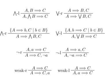
The sequent calculus G2 consists of the (axiom and) rules given in Figure 1.

a=⇒a A, B=⇒C V_-l A,V B =⇒C A=⇒B, C W_-r A=⇒W B, C {A=⇒b, C|b∈B} V -r A=⇒V B, C {A, b=⇒C|b∈B} W -l A,W B=⇒C A, a=⇒C ¬-r A=⇒C,¬a A=⇒a, C ¬-l A,¬a=⇒C A=⇒C weak-r A=⇒C, a A=⇒C weak-l A, a=⇒C

Figure 1: Sequent system G2

It is well known that this calculus is a sound, complete and (obviously) cut-free derivation system for the set of propositionally valid sequents.

Turning to one-sided sequent calculi for propositional logic, we first need to redesign the language by restricting the use of the negation symbol to proposition letters. That is, given a setPropof proposition letters, we define the setL∗₀(Prop) of propositional formulasin negation normal form, briefly: nnf-formulas, as follows:

a ::= p| ¬p|V A|W

A,

where p ∈ Prop, and A ∈ PωL0(Prop). A literal is a formula of the form p or ¬p, with

p ∈ Prop. Clearly every formula in L0(Prop) is equivalent to a formula in negation normal form. The one-sided sequent calculusG1 consists of the axiom scheme rules given in Figure 2. This calculus is a sound, complete and (obviously) cut-free derivation system for the set of propositionally valid one-sidedL∗₀-sequents.

p,¬p=⇒∅ A, B=⇒∅ V -l A,V B=⇒∅ {A, b=⇒_∅|b∈B} W -l A,W B=⇒∅ A=⇒∅ weak-l A, a=⇒∅

Figure 2: Sequent system G1

3

Moss’ coalgebraic logic

In this section we introduce the finitary version of Moss’ coalgebraic language. In the sequel, we deal with syntax mainly, and hence we are mostly concerned with thefinitary versions of the coalgebra functors. In order not to clutter up our notation too much, we often writeT

instead ofTω for brevity. 3.1 Syntax

The formulas of our language are inductively given as follows.

Definition 3.1 Given a set Prop of variables, the set L(Prop) of Moss formulas in Prop is given by the following grammar:

a ::= p| ¬a|V A|W

A| ∇α|∆α,

wherep ∈Prop, A∈ PωL(Prop) andα ∈ TωL(Prop). The fragmentL∗(Prop) ofL-formulas innegation normal form is defined as follows:

a ::= p| ¬p|V A|W

A| ∇α|∆α,

that is, we only allow negations in front of proposition letters. We will omit explicit reference to the set of proposition letters, for instance writing L rather thanL(Prop), if Propis either well known or not important.

Remark 3.2 In fact there are quite substantial differences between the language we just defined and Moss’ original language. First of all, Moss’ language does not have explicit proposition letters. Second, it is infinitary in nature, not only allowing infinite disjunctions but also expressions of the form∇αwithα an element ofTLrather than ofTωL. And finally, in his original language the modality ∆ does not occur. We feel justified to still refer to our syntax as (a variant of) Moss’ language because of the characteristic role of the∇modality. The connective ∆ should be understood as theBoolean dual of∇, in the same sense that

V

and W

are Boolean duals. For this purpose, consider the negation connective as a map ¬ : L → L mapping formulas to formulas. Applying the functor to this map we obtain a functionT¬ : TL → TL, so that for any α ∈ L, the expressions ∇(T¬)α and ∆(T¬)α are well-formed formulas. The point is now that the formula ∆αwill be equivalent to the formula

¬∇(T¬)α — following the analogy, observe that V

A ≡ ¬W

(P¬)A. The ∆ is discussed in detail in [10].

Despite its unconventional appearance, the languageL admits fairly standard definitions of most syntactic notions. The point of restricting Moss’ modality to the setTωL is that the formulas∇α and ∆αhave a finite, clearly defined set ofimmediate subformulas. To see this, recall from the preliminaries, that if α belongs to the set TωL, then the set Base(α) ∈PωL is the smallest (finite) subset X ⊆ L such that α ∈ TωX. This observation underlies the following syntactic definitions.

Definition 3.3 The setSfor(a) ofsubformulas of a Moss formulaais inductively defined as follows: Sfor(p) := {p} Sfor(¬a) := {¬a} ∪Sfor(a) Sfor(A) := {A} ∪ S a∈A Sfor(a) ( ∈ {V ,W_} ) Sfor(♥α) := {♥α} ∪ S a∈Base(α) Sfor(a). (♥ ∈ {∇,∆})

The elements ofBase(α)⊆Sfor(∇α) will be called theimmediate subformulas of ∇α. The (modal) depth d(a) of a Moss formula ais inductively defined as follows:

d(p) := 0 d(¬a) := d(a) d(A) := max(d[A]) ( ∈ {V ,W }) d(♥α) := 1 + max d[Base(α)] (♥ ∈ {∇,∆}) It is not hard to see that Sfor(a) is a finite set and that d : L → ω is well-defined map assigning to each formula aa natural numberd(a).

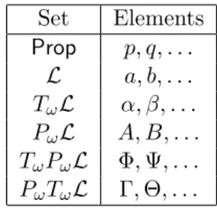
Convention 3.4 Since in this paper we will not only be dealing with formulas and sets of formulas, but also with elements of the setsTωL,PωTωLand TωPωL, it will be convenient to use the naming convention of Figure 3. Observe that, similar to taking negation as a map

Set Elements Prop p, q, . . . L a, b, . . . TωL α, β, . . . PωL A, B, . . . TωPωL Φ,Ψ, . . . PωTωL Γ,Θ, . . .

Figure 3: Naming convention ¬:L → L, we may see the boolean connectivesW

andV

to formulas, W ,V

: PωL → L. Applying the functor to these maps, we obtain functions

TW

, TV

:TωPωL → TL. In particular, for any object Φ ∈ TωPωL, we obtain well-formed formulas of the form∇(TW

)Φ and∇(TV

)Φ. 3.2 Semantics

Since we included explicit proposition letters in our language, we have to interpret our formu-las inT-models, that is,T-coalgebras that are endowed with a valuation function interpreting the proposition letters.

Definition 3.5 A valuation on a T-coalgebra (S, σ) is a valuation V : Prop → P S; the induced structure (S, σ, V) will be called a T-model or coalgebraic model. For such a model, the satisfaction relationσ,V ⊆S× L is defined by the following induction on the complexity of formulas: sσ,V p if s∈V(p), sσ,V ¬a if s6σ,V a, sσ,V VA if sσ,V afor all a∈A, sσ,V W A if sσ,V afor somea∈A, sσ,V ∇α if (σ(s), α)∈T(σ,V), sσ,V ∆α if (σ(s), α)6∈T(6σ,V),

Ifs σ,V a we say that ais true, or holds ats in S, and we usually write S, s a, where S

denotes the T-model (S, σ, V). When no confusion is likely we may write s a instead of

S, sa.

Remark 3.6 For those readers that are worried about the correctness of this definition we note that given the properties of relation lifting, the clause for the∇modality may be replaced with the following:

sσ,V ∇α if (σ(s), α)∈T(σ,VS×Base(α)),

which reveals the inductive nature of the definition: in order to know whether∇α is true at a points, we only need to know the meaning of the immediate subformulas of∇α. A similar observation can be made about ∆.

The semantics of the ∆-operator is perhaps easier to understand by observing that the formula ∆α is false at a states iff the pair (σ(s), α) belongs to the lifted version T6of the complement 6of the satisfaction relation.

Example 3.7 For the binary tree functorId×Id, the semantics of nabla is as follows: given

α = (a0, a1), a coalgebra σ: X→X×X and a state swithσ(s) = (t0, t1)

s∇(a0, a1) ifft0 a0 and t1 a1.

Example 3.8 For the powerset functorP, the semantics of nabla in a coalgebraσ: X→P X

and a statesis

s∇α iff (∀a∈α)(∃t∈σ(s)) sa

Example 3.9 For the bag (multiset) functor B nabla works as follows. Recall from the previous section that we may represent a multiset α : L → _N by its positive graph, it is a usefull notation to write it as follows: {aα(a)|a∈ L}. Given a coalgebraσ: X →BX and a states, the condition forsσ ∇α unravels as follows (for the definition of lifting in this case see Example 2.11):

sσ ∇α iff ∃x∈B() such that ∀t: σ(s)(t) = P {a|ta}

x(t, a)

and ∀a: α(a) = P

{t|ta}

x(t, a). (13)

For example, if σ(s)(t1) = 5, σ(s)(t2) = 3 and σ(s)(t3) = 2 and t1aand t2, t3b, it is easy to see that

s∇{a5, b5}.

Two important observations about finitary Moss’ logic are that it isadequate with respect to behavioral equivalence (or, equivalently, bisimilarity), and expressive when we confine attention to finitely branching coalgebras. For this purpose, given two T-models S and S0,

with states sand s0, respectively, we write S, s≡LS0, s0 to indicate that for all L-formulas a

we have S, s aiff S0, s0 a. We call a coalgebra (S, σ) finitely branching if σ :S → TωS, that is, the range ofσ is included in the setTωS.

Fact 3.10 Let S = (S, σ, V) and S0 = (S0, σ0, V0) be two T-models with states s and s0,

respectively.

1. L is adequate: if S, s↔S0, s0 then S, s≡LS0, s0

2. L is finitely expressive: if S, s ≡L S0, s0 then S, s ↔ S0, s0, provided that σ and σ0 are

finitely branching.

The same holds for the∆-free fragment of the language.

Definition 3.11 We say that a formula a entails a formula b, notation: a≤ b, if for every coalgebraic modelS= (S, σ, V), and anys∈S, we have that wheneverS, sathenS, sb.

We say that two formulas a and b are equivalent, notation: a ≡ b, if a ≤ b and b ≤ a. A formulaaisvalid, notation: |=a, if it holds at every state of every coalgebraic model.

Example 3.12 It is easy to prove that nabla is a monotone modality in the following sense:

αT(≤)β entails ∇α≤ ∇β.

This is the rule∇1 of the the derivation system M[11].

Example 3.13 Recall from the discussion in Convention 3.4 that for every Φ∈TωPωL, we may consider the (correctly defined) formula∇(TW

)Φ. For such a Φ it is straightforward to verify that the set λT(Φ) ∈ P TL actually belongs to the set PωTωL, so that Φ has finitely

many lifted members, all belonging to the setTωL. This means that the expression W

{∇α|

α ∈λT(Φ)} is actually a well-formed formula. It happens to be the case that ∇(TW

)Φ≡_{∇α|α ∈λT(Φ)}. (14) The corresponding equation is, under the name (∇3), a key axiom of the derivation system

M [11].

For a good understanding of the semantics of our language, and of the sequent calculi to be defined later on, we need to discuss the relation between ∇and ∆ in somewhat more detail. We already mentioned that ∆ can be seen as the Boolean dual of ∇— this can now be made precise, see Fact 3.15. In addition however, perhaps surprisingly, the semantics of ∆ can also be expressed in terms of∇without the use of the negation. For this purpose, we need the following definition.

Definition 3.14 Forα inTωL, we put

D(α) := Φ∈T PBase(α)|(α,Φ)∈/ T6∈ , LT(α) := {(TV)Φ|Φ∈ D(α)},

RT(α) := {(TW)Φ|Φ∈ D(α)}.

Fact 3.15 [10] LetS= (S, σ, V) be a coalgebraic model, andsa state in S. For anyα∈TωL

the following equivalences hold:

S, s∆α iff S, s¬∇(T¬)α iff S, s∇β for some β∈LT(α) (15)

and

S, s∇α iff S, s¬∆(T¬)α iff S, s∆β for all β∈RT(α). (16) While for the powerset functor we consequently simplify the definition of LT and RT, for the other functors the ”double negation” definition of the set D(α) might seem cryptic. Therefore, recalling the definition of the relation lifting, we illustrate the above definition with the bag functorB:

Example 3.16 Consider a multiset{an}. Then

RB({an}) ={(B

_

)Φ |Φ :P{a∨b} →N, ¬({an}B(∈/)Φ)},

where the condition for Φ actually means that either Φ(∅) 6= n or Φ({a}) > 0. Thus

RB({an}) ={{⊥k}|k6=n} ∪ {{am}|m >0}.

Remark 3.17 Clearly, on the basis of the previous fact, we may see ∆ as a definable con-nective in the language with∇as the only modality, by putting ∆α:=¬∇(T¬)α.

The reader may also be tempted to conclude, that we can define ∆ in terms of the connectives ∇,V

and W

alone (that is, without using negation), via ∆α := W

{∇β | β ∈

LT(α)}. The problem is, however, that unless the functor T restricts to finite sets, the setsD(α) and LT(α) may beinfinite (asRB({an}) in the example above); in that case, the

proposed defining expressionW

{∇β |β ∈LT(α)}is not a well-formed formula of our language. Nevertheless, in caseT does restrict to finite sets, the formulas ∆α and W_{∇

β |β ∈LT(α)} are equivalent, and so are∇α and V

{∆β |β ∈RT(α)}.

We now turn to the notion of a valid sequent, which we define in a completely standard way. Intuitively, a sequent A=⇒ B is valid iff the formulaV

A→ W

B holds in every state of every coalgebraic model.

Definition 3.18 A sequentA =⇒B isvalid, notation: |=A=⇒B, if for every coalgebraic model S= (S, σ, V), and any s∈ S, the following holds: whenever S, s a for all formulas

a∈A, then there is at least one formula b∈B such that S, sb. If the above condition fails

we say that the sequentA=⇒B is refuted atsinS, and we say thatA=⇒B isrefutable if

it can be refuted somewhere.

Clearly then a sequent is not valid iff it is refutable. 3.3 Slim redistributions

An important role in this paper is played by the notion of a slim redistribution, and its variant of aseparated slim redistribution. Slim redistributions are the key to understand how ∇ interacts with V

; and as we will see, separated slim redistributions enable us to use the same idea in a setting of two-sided sequent systems.

Remark 3.19 Formulated specifically for the power set functor, that is, in the case that

T = P, a set Φ ∈ T P X is a slim redistribution of a set Γ ∈ P T X iff S

Γ = S

Φ and

F∩α6=∅for all F ∈Φ and γ ∈Γ. (We keepT and P separated in the notation in order to

facilitate the abstraction to the general case.) Borrowing some intuition from topology, these two conditions tell us that on the one hand every givenγ ∈Γ is ‘covered’ by Φ (in the sense that γ ⊆ S

Φ) in such a way that every F ∈ Φ has nonempty intersection with γ. On the other hand, the requirement thatS

Φ⊆S

Γ is a minimality condition on Φ, taking care that every such Φ can be effectively constructed from Γ by scrambling and suitably reorganizing its ‘ingredients’.

The above relation between Φ and Γ can be reformulated in terms of the lifted membership relationT∈. Recall that γ ∈T X is a lifted member of Φ∈T P X ifγ ⊆S

Φ and γ∩F 6=∅

for allF ∈Φ. Hence we will say that Φ is a redistribution of Γ if Γ⊆λP(Φ) (every element of Γ is a lifted member of Φ), and that Φ is slim if Φ⊆T P(S

Γ) (Φ is built from the ingredients of Γ). It is this formulation that can be generalized to the case of an arbitrary set functor.

Definition 3.20 A set Φ ∈ T P X is a redistribution of Γ ∈ P T X if Γ ⊆ λT_X(Φ). In case Γ ∈ PωTωX, we call a redistribution Φ slim if Φ ∈ TωPω(Sα∈ΓBase(α)). The set of slim redistributions of Γ is denoted asSRD(Γ).

For brevity, in the sequel we will often write B(Γ) instead ofS

γ∈ΓBase(γ).

Example 3.21 Consider the powerset functor: the following are simple examples of the set of slim redistributions • SRD({{a0}. . .{an}}) ={{a0, . . . , an}} • SRD({{a}}) ={{a}} • SRD({_∅}) ={_∅} • SRD({α,∅}) =∅ifα6=∅ • SRD(∅) =P∅

It holds in general that

SRD(∅) =T∅.

Example 3.22 To see how slim redistributions are involved in the interaction between∇and

V

, consider an arbitrary collection of formulas V_{∇

γ |γ ∈ Γ} for some finite set Γ⊆ TωL. A straightforward argument suffices to show that the following holds, for anyT-modelS and

any state inS:

S, s∇γ for all γ ∈Γ iffS, s∇(TV)Φ for some Φ∈SRD(Γ). (17)

In the case thatT restricts to finite sets, the setSRD(Γ) is finite, and we may formulate (17) as an equivalence of formulas:

^

{∇γ |γ ∈Γ} ≡_{∇(TV

)Φ|Φ∈SRD(Γ)}.

Formulated as the derivation rule (∇2), the equivalence (17) provides one of the key principles underlying the derivation systemM [11].

In the setting of two-sided sequent calculi, we need to slightly modify the notion of a slim redistribution. For an intuitive explanation of the required modification, suppose that we are dealing with a sequent of the form {∇γ | γ ∈ Γ} =⇒ {∆θ | θ ∈ Θ}, and that we want to introduce a proof rule to reduce this sequent. Using the fact that ∆ is the Boolean dual of ∇, we may think of this sequent as the one-sided {∇γ | γ ∈ Γ},{∇(T¬)θ | θ ∈ Θ} =⇒ _∅, corresponding to the conjunction ^ {∇γ | γ ∈ Γ} ∪ {∇(T¬)θ | θ ∈ Θ}. A natural way to reduce this sequent would be to use the equivalence (17), working with the set

SRD Γ∪(T¬)[Θ]

. However, this leads to problems in case the sets Γ and (T¬)[Θ] overlap: we need to remember which side of the sequent the objectsγ (left) or (T¬)θ(right) originally came from. Formally, our way of dealing with this kind of sequent is the following.

Definition 3.23 Given Γ,Θ∈PωTωL, let

B0_{(Γ) :={(a,0)|a∈ B(Γ)}, B}1_{(Θ) :={(b,1)|b∈ B(Θ)},}

and let the assignments a 7→ (a,0) and b 7→ (b,1) define the maps f0 : B(Γ) → B0(Γ) and

f1:B(Θ)→ B1(Θ) respectively. We identify the disjoint unionB(Γ)]B(Θ) withB0(Γ)∪B1(Θ) withf0, f1 as the injection maps. Then define the set of separated slim redistributions of Γ

andΘ as follows: SSRD(Γ,Θ) := n Φ∈T P(B(Γ)] B(Θ))| ∀α∈Γ (T f0)α T∈Φ) &∀β ∈Θ (T f1)β T∈Φ) o .

Given a Φ∈SSRD(Γ,Θ), any A∈Base(Φ) is a subset ofB(Γ)] B(Θ), and so we may define the setsAL, AR∈PωL by putting

AL:= ( ˘P f0)Aand AR:= ( ˘P f1)A, (18) where ˘P denotes the contravariant power set functor. In order to provide some intuition concerning the above definition of the setsALand AR, we mention (without proof) that for any Φ∈SSRD(Γ,Θ), the sets (TP f˘ 0)Φ and (TP f˘ 1)Φ are slim redistributions of Γ and Θ, respectively, and for anyA∈Base(Φ), the setsAL and

AR are elements ofBase((TP f˘ 0)Φ) and Base((TP f˘ 1)Φ), respectively. As a consequence, we find thatAL⊆ B(Γ) and AR⊆ B(Θ); in particular, if we think of the sequent AL=⇒ARas being formed by{∇α |α ∈Γ}=⇒ {∆β |β ∈Θ}, we may observe that material originating from the given side (left or right) of the latter sequent will end again on that same side.

The definition ofSSRD and its intuition coming from dealing with sequents which have two sides is further motivated by the following key example:

Example 3.24 A key example of a separated slim redistribution of sets Γ,Θ∈TωPωLarises semantically. Fix a modelSand a state sinS. Consider, for any state tof S, the set

Qt:=

f0a|a∈ B(Γ) andS, ta ∪f1b|b∈ B(Θ) and S, t6b .

This defines a map Q : S → P(B(Γ)] B(Θ)), and hence applying the functor we obtain a mapT Q:T S→T P(B(Γ)] B(Θ)) Then for the object Φs:= (T Q)(σ(s))∈T P(B(Γ)] B(Θ)) one may prove

Φs∈SSRD(Γ,Θ) iffS, s∇α for all α∈Γ andS, s6∆β for all β ∈Θ. (19)

We do not prove this fact here since it resembles the proof of Lemma 5.2.

Example 3.25 For the binary tree functor Id ×Id, consider a nonempty set of pairs, e.g. Γ ={(a0, a1),(b0, b1)}, then SRD(Γ) ={(A, B) | {a0, b0} ⊆ A,{a1, b1} ⊆ B} where A, B ∈

Pω(Base(α)∪Base(β)).

Similarly for SSRD(Γ,Σ) in case one of the sets is nonempty. SRD(∅) =SSRD(∅,∅) = ∅×∅=∅.

Example 3.26 We list some simple examples of SSRD for the powerset functor, some of them appear later in the examples of proofs:

• SSRD(∅,∅) =P∅

• SSRD({∅},{∅}) ={∅}

• SSRD({α,∅},Σ) =∅whenever α6=∅, or Σ6=∅and Σ6={∅}

• SSRD(∅,{{a}}) ={{(a,1)}}

Example 3.27 For the bag functor B we compute SSRD({a5, b5},{⊥n_{}) where n6= 10: it} is empty, there is no such SSRD. For suppose there is some Φ :Pω{(a,0),(b,0)(⊥,1)} →N

with {(a,0)5,(b,0)5} B∈ Φ and at the same time {(⊥,1)n} B∈ Φ. This would mean we have at the same time witnesses x0 and x1 in B(∈) for these two facts. Imagine we are filling the ”witness squares” simultaneously: the bases of the two multisets are disjoint, thus for each A ∈ Pω{(a,0),(b,0)(⊥,1)} not containing (⊥,1) we have to fill x1(a, A) = 0 and x1(b, A) = 0, and for each A not containing (a,0) nor (b,0) we similarly have to fill

x0(⊥, A) = 0, and consequently for any of these sets we must have Φ(A) = 0. Now for the rest of sets A ∈ Pω{(a,0),(b,0)(⊥,1)} — those containing (⊥,1) and at the same time containing (a,0) or (b,0) — it holds that

X x0(⊥, A) = X x1(a, A) + X x1(b, A) = 10 = X Φ(A) which givesP

Φ(A) = 10 contradicting the fact that{(⊥,1)n}B∈Φ andn6= 10.

4

The case of the power set functor

Throughout this section we assume that T = P, that is we are dealing with the power set functor. As a consequence, Tω is the finitary power set functorPω.

We will first introduce a two-sided sequent system S2P for the full language LP, and then a one-sided system S1P for the variant L∗P of the language where the use of negation is restricted to atomic formulas. These two systems are simplified versionsof the corresponding instances of the proof systems G2T,G1T, which we will define in the next section.

4.1 The sequent calculus S2P

In order to define the two-sided calculusS2P, we introduce the following variants of the sets

LT(α) and RT(α) of Definition 3.14.

Definition 4.1 For everyα∈TωL let us define

L0_Pα= ( {{_∅} ∪ {{a} |a∈α} ∪ {{V α,>}}} ifα6=∅ {{>}} ifα=∅ (20) R0_Pα= ( {{_∅} ∪ {{a} |a∈α} ∪ {{W α,⊥}}} ifα6=∅ {{⊥}} ifα=∅ (21)

Remark 4.2 Note thatL0_P(α) andR0_P(α) arenot the sets we obtain by instantiatingT =P

in the definition ofLT(α) and RP(α) of Definition 3.14. We leave it for the reader to verify that L0_P(α) ⊆ LP(α), and that in general it is a proper subset. It is in this sense that the systemS2P simplifies the calculusG2T defined in the next section.

The importance of these notions is that they allow us to interdefine ∇ and ∆, without the use of the negation operator.

Lemma 4.3 For every α, β ∈TωL,

∆α≡_{∇β|β ∈L0_Pα} ∇α≡^{∆β|β ∈R0_Pα}.

Proof. We omit the proof of this Lemma, which is a routine verification. qed We are now ready to introduce the calculusS2P. It extends the propositional calculusG2 with two kinds of modal proof rules. The rules ∆-l and∇-r can be seen as the incarnation of the previous lemma into proof rules. For a motivation of the last rule of the system,P(∇∆), which reduces the modal depth of sequents, we refer to the subsection on separated slim redistributions.

Definition 4.4 The sequent calculusS2P for the language LP is defined as the extension of the propositional calculusG2 with the following modal rules:

{A,∇β =⇒B |β∈L0_Pα} ∆-l _A,∆α=⇒B {A=⇒∆β, B|β∈R 0 Pα} ∇-r _{A=⇒ ∇α, B} {AΦ_L =⇒A_RΦ |Φ∈SSRD(Γ,Σ)} P(∇∆) _{{∇α|α∈Γ}=⇒ {∆β |β∈Σ}} ∀Φ. AΦ∈Φ

The rule P(∇∆) is to be read as follows: given Γ,Σ∈PωTωL, if for every Φ∈SSRD(Γ,Σ) there exists someAΦ∈Φ such thatAΦ_L=⇒AΦ_R, then{∇α|α∈Γ}=⇒ {∆β |β ∈Γ}. The following lemma states soundness of theP(∇∆) rule: whenever the side condition is satisfied and the resulting assumptions are valid sequents, the conclusion is a valid sequent as well. But it also states a form of invertibility of the rule: whenever the conclusion is valid we can find suitable valid assumption sequents fulfilling the side condition. The lemma is for convenience stated as a contraposition:

Lemma 4.5 The following are equivalent for all Γ,Σ ∈ PωTωL and all finite sets C, D of

proposition letters:

1. the sequent{∇α|α∈Γ}, C =⇒D,{∆β |β∈Σ} is not valid.

2. the sequent C =⇒ D is not valid, and for some Φ ∈ SSRD(Γ,Σ), AL =⇒ AR is not

Proof. Let us show that (1) implies (2): By assumption,C =⇒Dis not valid and there exists a modelSand a statesinSsuch thatS, s∇αfor everyα∈Γ andS, s6∆βfor everyβ∈Σ.

For every t∈R[s], let At:= {f0a|a∈SΓ and S, ta} ∪ {f1b|b∈SΣ andS, t6b}, and

let Φs ={At|t∈R[s]}. By definition, AL=⇒ AR is not valid for allA ∈Φs, and we have already checked that Φs∈SSRD(Γ,Σ) (see Example 3.24).

Conversely, assume thatC =⇒ D is not valid (hence, C∩D=∅) and that there exists

some Φ ∈ SSRD(Γ,Σ) such that for every A ∈Φ, AL =⇒AR is not satisfied at some state

sA in some model SA. Then consider the model S which consists of the disjoint union of the

modelsSAplus one extra pointssuch thatR[s] ={sA|A∈Φ}and p∈V(s) iffp∈C. It is routine to verify that S, ssatisfies{∇α|α∈Γ} ∪C∪ {¬∆β|β ∈Σ} ∪ {¬p|p∈D}. qed

Theorem 4.8 below states the soundness and completeness of S2P (with respect to the standard semantics). Since S2P is formulated without the cut rule, once completeness has been established, it immediately follows that the cut rule is redundant.

To be able to perform an inductive argument we introduce a measure on sequents. The measure is induced by the modal depth of formulas as given in Definition 3.3, and by a measure of left and right formula occurrences in the sequent.

Definition 4.6 By induction on the complexity of a formulaainLP we define the following measures kl(a), kr(a): kl(p) := 1 kr(p) := 1 kl(¬a) := 1 +kr(a) kr(¬a) := 1 +kl(a) kl(A) := 1 + P a∈A kl(a) kl(A) := 1 + P a∈A kl(a) ( ∈ {V,W}) kl(∇α) := 2 kr(∇α) := 3 kl(∆α) := 3 kr(∆α) := 2

Finally, given a sequent A=⇒B, we let

m(A=⇒B) :=max(d[A∪B]),X a∈A kl(a) + X b∈B kr(b)

denote its measure.

Intuitively, kl(a) and kr(a) measure the boolean complexity of a occurring on the left side (right side) of a sequent, where formulas of the form ∇α and ∆α count as proposition letters with a slightly enlarged weight. The full measure of a sequent being a pair of natural numbers, we will order the setω×ω lexicographically, that is:

(m, n)<(m, n0) if m < m0 orm=n andn < n0.

As we will see in the proof below, with this definition we ensure that for each rule the complexity of any of its assumptions is strictly less than that of its conclusion.

Lemma 4.7 For each rule of the calculus S2P, the measure of any of its assumptions is

Proof. Let us denotem(A=⇒B) by (k, l). We show that in a backward application of the

P(∇,∆) rule, kstrictly decreases, and that for all the other rules k does not increase, while

lstrictly decreases.

Leaving the propositional rules as an exercise for the reader, we consider the modal rules explicitly. For the ∆-l rule, denote P

a∈A

kl(a) + P b∈B

kr(b) =n. Now m(∆α, A=⇒ B) = 3 +n while m(∇β, A =⇒ B) = 2 +n. Since the modal depth clearly remains unchanged, this suffices for the ∆-l rule. Clearly, the case of the ∇-r rule is similar.

Consider a backward application of theP(∇,∆) rule. From the definition of Φ∈SSRD(Γ,Σ) and ofAΦ_L and AΦ_R it is clear that the modal depth of each assumption (that is, max(d[AΦ_L∪

AΦ_R])) is strictly less then that of the conclusion. qed

Theorem 4.8 (Soundness and Completeness ofS2P) For everyLP-sequent A=⇒B, `_S2P A=⇒B iff |=A=⇒B.

Proof. The proof of soundness is standard, by induction on the depth of the derivation of

A =⇒B. The only cases of interest are when the last rule applied is (a) ∆-l, (b) ∇-r or (c)

P(∇∆). The cases (a) and (b) readily follow from Lemma 4.3. Case (c) follows from the implication (1 =⇒ 2) of Lemma 4.5.

As for completeness, it is shown by induction on the m(A =⇒ B). If m(A =⇒ B) = (0,0) thenA=B =∅and the sequent is not valid (and by soundness it is also not provable.)

The induction step for a sequentA=⇒B with m(A=⇒B)6= (0,0) distinguishes two cases: either the sequent is of the form {∇α |α ∈Γ}, C =⇒ D,{∆β |β ∈Σ} where C, D are sets of proposition letters (which we call a reduced form), or it is not.

Case 1. The sequent A =⇒ B is not of the reduced form. Observe that the propositional rules and the∇-r and ∆-l rules are invertible, that is, they preserve validity backwards (the latter two by Lemma 4.3). Moreover, with each backwards application of any of the mentioned rules, the value of m(A =⇒ B) strictly decreases by Lemma 4.7. It is then clear then we can apply the mentioned rules backwards until no such rule is applicable, and this procedure terminates in a set of sequents {Ai =⇒ Bi |i ∈ I}, each of them (a) being of the reduced form, (b) having a strictly smaller measure than the sequent we started with, and (c) being valid. To show that the sequentA =⇒B is provable, we apply the induction hypothesis to the sequents Ai =⇒ Bi, and finish the proof with the applications of the appropriate rules forward.

Case 2. The sequent A =⇒ B is of the reduced form, say {∇α |α ∈ Γ}, C =⇒ D,{∆β |

β∈Σ} whereC, D are sets of atoms. From the assumptions and the implication (2 ⇒ 1) of Lemma 4.5, we obtain one of the following two subcases.

Subcase 2a. The propositional sequentC=⇒Dis valid, in which casep∈C∩Dfor some proposition letterp. Then we can start a derivation with the axiom p =⇒ p as its only leaf followed by applications of the weakening rules to derive the full sequentA=⇒B.

Subcase 2b. For each Φ∈SSRD(Γ,Σ) there exists some setAΦ ∈Φ such that the sequent

AΦ

can apply the induction hypothesis and conclude that for each Φ∈SSRD(Γ,Σ) the sequent

AΦ_L =⇒ AΦ_R is provable. Then we may obtain a derivation for our sequent by prolonging all these derivations with an application ofP(∇∆), so as to obtain a proof of{∇α|α∈Γ}=⇒ {∆β |β ∈Σ}, followed by applications of left and right weakening rules to add the elements

inC and Drespectively. qed

Example 4.9 We illustrate the modal rules of the calculus with the following simple proof of one of the original nabla axioms:

∅ P(∇,∆) ∅=⇒∆{⊥},∆∅ ∅=⇒ > P(∇,∆) ∅=⇒∆{>} ∅=⇒ > ∅=⇒ >,⊥ P(∇,∆) ∅=⇒∆{>,⊥} ∇-r ∅=⇒∆{⊥},∇{>} ∇-r ∅=⇒ ∇∅,∇{>}

Here the following is needed to see that the above is a correct proof: • R0_P(∅) ={{⊥}} for the last inference

• R0_P({>}) ={_∅,{>},{>,⊥}}for the one but last inference • SSRD(∅,{{⊥},∅}) =∅

• SSRD(∅,{{>}}) ={{(>,1)}}

• If Φ∈SSRD(∅,{{>,⊥}}) then either{(>,1)} ∈Φ or {(>,1),(⊥,1)} ∈Φ

Example 4.10 As another example we prove the sequent ∇{a},∇{b}=⇒ ∇{a, b}. In this case we use the fact that R0_P({a, b}) = {∅,{a},{b},{a∨b,⊥}}. To derive this sequent we

have to prove the following four sequents: First, ∅ P(∇,∆) ∇{a},∇{b}=⇒∆∅ is provable becauseSSRD({{a},{b}},{_∅}) =∅. Second, a, b=⇒a P(∇,∆) ∇{a},∇{b}=⇒∆{a}

is provable because the only member ofSSRD({{a},{b}},{{a}}) is{{(a,0),(b,0),(a,1)}}. Third, a, b=⇒b P(∇,∆) ∇{a},∇{b}=⇒∆{b} similarly as above. And fourth,

a, b=⇒a∨b a, b=⇒a∨b,⊥

P(∇,∆)

∇{a},∇{b}=⇒∆{a∨b,⊥}

is correct because for each Φ∈SSRD({{a},{b}},{{a∨b,⊥}}) we have either{(a,0),(b,0),(a∨

b,1)} ∈Base(Φ) or{(a,0),(b,0),(a∨b,1),(⊥,1)} ∈Base(Φ), thus fulfilling the side condition of the rule. Example 4.11 ∅ P(∇,∆) ∇∅=⇒∆{a,⊥} a=⇒a a=⇒a,⊥ P(∇,∆) ∇{a}=⇒∆{a,⊥} ∇∅∨ ∇{a}=⇒∆{a,⊥}

where in the left branch the set SSRD({∅},{{a,⊥}}) = ∅. In the other branch

ob-serve that for each Φ∈ SSRD({{a}},{{a,⊥}}) we have either {(a,0),(a,1)} ∈ Base(Φ) or {(a,0),(a,1),(⊥,1)} ∈Base(Φ).

Example 4.12 As the last example we give a cut free proof of the sequent, which has been shown in Remark 27. of [6] to have no cut free proof in the calculus introduced there. The following four proof trees prove four assumptions of the last∇-r inference:

∅ ∇{p∨q}=⇒∆∅ ∅ ∇{p∨q}=⇒∆∅,∆{q,>} ∅ ∇{p∨q}=⇒∆∅,∆{q} ∇-r ∇{p∨q}=⇒∆∅,∇{q} ∅ ∇{p∨q}=⇒∆∅ ∇{p∨q}=⇒∆∅,∆{p} p∨q=⇒p, q ∇{p∨q}=⇒∆{p},∆{q} p∨q=⇒p, q,> p∨q=⇒p, q p∨q=⇒p,> ∇{p∨q}=⇒∆{p},∆{q,>} ∇-r ∇{p∨q}=⇒∆{p},∇{q} ∅ ∇{p∨q}=⇒∆∅ ∇{p∨q}=⇒∆∅,∆{>} p∨q=⇒ >, q ∇{p∨q}=⇒∆{>},∆{q} p∨q=⇒ >, q ∇{p∨q}=⇒∆{>},∆{q,>} ∇-r ∇{p∨q}=⇒∆{>},∇{q} ∅ ∇{p∨q}=⇒∆∅ ∇{p∨q}=⇒∆∅,∆{p∨ >,⊥} p∨q=⇒ > ∨p, q p∨q=⇒ > ∨p, q,⊥ ∇{p∨q}=⇒∆{p∨ >,⊥},∆{q} p∨q=⇒ > ∨p, q p∨q=⇒ > ∨p, q,⊥ ∇{p∨q}=⇒∆{p∨ >,⊥},∆{q,⊥} ∇-r ∇{p∨q}=⇒∆{p∨ >,⊥},∇{q}

where in the last proof tree we use a compact notation for space reasons: the two top sequents in the middle constitute the two assumptions of the inference, the same applies to the two top sequents on the right.

Next, one ∇-r inference applied to the four conclusions of the four proof trees above yields: ∇{p∨q}=⇒ ∇{p,>},∇{q}.

The conditions are not hard to check, e.g.

RT({p,>}) ={∅,{p},{>},{p∨ >,⊥}}

and in the last proof tree each Φ∈SSRD({{p∨q}},{{p∨ >,⊥},{q,⊥}}) must contain either {(p∨q,0),(> ∨p,1),(q,1)} or{(p∨q,0),(> ∨p,1),(q,1),(⊥,1)}.

4.2 The sequent calculus S1P

Let us now introduce the cut free, one-sided sequent proof system S1P, which arises from the classical propositional left-sided calculus G1 (introduced in Section 2) by adding modal rules.

The language for this calculus is the restriction L∗ of L where negations can only be applied to proposition letters. Every formula inLis semantically equivalent to some formula of L∗. One way to see this is to recall that the nabla operator is interdefinable with the standard modal operators 2 and 3, and that every formula of the basic modal language is equivalent to a formula in which negations can only be applied to proposition letters. Sequents for this calculus are of form A=⇒∅, where Ais a finite set of formulas in L∗.

Definition 4.13 The calculus S1P, operating on L∗_P-sequents, is obtained by extending the calculus G1 with the following modal rules:

{A,∇β =⇒_∅|β ∈L0_Pα} ∆-l ∆α, A=⇒∅ {AΦ =⇒_∅|Φ∈SRD(Γ)} P(∇) _{{∇α|α∈Γ}=⇒} ∀Φ.AΦ ∈Φ ∅

The rule P(∇) is to be read as follows: given Γ ∈ PωTωL, if for every Φ ∈ SRD(Γ) there exists some AΦ∈Φ such that AΦ=⇒_∅, then{∇α|α∈Γ}=⇒_∅. Recall that a sequent A =⇒ ∅ is valid if A is not satisfiable, i.e. for every model S and

every statesinS, there exists somea∈A such thatS, s6a. Then the next lemma provides

the soundness and a form of semantic invertibility of the rule P(∇):

Lemma 4.14 The following are equivalent for every Γ ∈ PωTωL and every collection C of

literals:

1. {∇α|α∈Γ} ∪C is satisfiable;

2. C is satisfiable and there is someΦ∈SRD(Γ) such that every A∈Φ is satisfiable. Proof. The proof of this lemma can be verified directly, or by unravelling the meaning of equation (17) in Example 3.22 for the case T =P. qed

The following theorem states the soundness and completeness ofS1P.

Theorem 4.15 (Soundness and completeness for S1P) For each L∗-sequentA=⇒∅,

Proof. The soundness follows from the soundness of the calculusS2P, because the one-sided rules are in fact just instances of the corresponding two-sided rules.

As for completeness, we use the measure m(A =⇒ ∅) defined previously, and reason

by induction on this measure. It obviously decreases with each backward application of a one-sided rule.

Ifm(A=⇒ ∅) = (0,0), then A=∅ and the sequent is not valid (and by soundness also

not derivable.)

Suppose that m(A=⇒_∅)>(0,0). As in the two-sided case, the propositional rules and the ∆-l rule are invertible. Thus the only interesting case is to consider a sequent which is of the form {∇α | α ∈ Γ} ∪C =⇒ _∅ where C is a finite collection of literals. From the assumptions it follows that the set {∇α | α ∈ Γ} ∪C is not satisfiable, and to by the implication (2 =⇒ 1) of Lemma 4.14, there are two possibilities: either C is not satisfiable, or for every Φ∈SRD(Γ) there exists someAΦ ∈Φ which is not satisfiable.

If C is not satisfiable, then there is some atom p ∈ C with ¬p ∈ C. We produce a derivation, starting with the axiom p,¬p =⇒ ∅, and continuing with applications of the

weakening rule to derive{∇α|α∈Γ} ∪C =⇒_∅.

On the other hand, suppose that C is satisfiable and that for every Φ ∈ SRD(Γ) there exists some AΦ ∈ Φ such that |= AΦ =⇒ ∅. Then by induction hypothesis we have

`S1P A

Φ _=⇒

∅ for every Φ ∈ SRD(Γ). Then a derivation for our sequent consists of

the prolongation of all these derivations, taken together, with an application ofP(∇), so as to obtain a proof of{∇α |α ∈ Γ} =⇒ ∅, followed by applications of weakening to add the

elements inC. qed

Example 4.16 We illustrate the modal rules of the one-sided calculus with a simple proof: ⊥=⇒_∅

P(∇,∆)

∇{⊥}=⇒∅

where the only member of SRD({{⊥}}) is{{⊥}}. 4.3 The ∆-free fragment

Since the modality ∆P is definable in the ∆P-free fragment ofL∗(recall Lemma 4.3) it makes sense to restrict ourselves to this fragment without loosing expressive power. The setting we have used so far is modular: we can obtain a complete one-sided calculus S1P∇ for the Delta-free fragment of the language simply omitting the ∆-l rule in the previous calculusS1P:

Definition 4.17 The calculus S1P∇, operating on ∆P-free L∗P-sequents, is obtained by ex-tending the calculusG1 with the following modal rule:

{AΦ =⇒∅|Φ∈SRD(Γ)}

P(∇) _{{∇α|α∈Γ}=⇒} ∀Φ.AΦ ∈Φ

∅

The proof of the following theorem is then immediately obtained from the earlier proofs:

Theorem 4.18 (Soundness and completeness for S1P∇) For each ∆-free L∗-sequent

A=⇒_∅,

`S1P A=⇒∅ iff |=A=⇒∅.

5

The general case

We have now arrived at the main section of our paper, where we will discuss sequent calculi for finitary Moss’ coalgebraic language in the case of a general finitary coalgebra functor

T (satisfying our default constraints of preserving inclusions and weak pullbacks). More specifically, we will define two-sided sequent system G2T for the full language, and a one-sided systemG1T for the version of the language where negation may only occur in front of proposition letters.

5.1 The two-sided sequent calculus G2T

For the introduction of the two-sided systemG2T, the reader should recall that we defined the setsLTα andRTαin Definition 3.14 (and explained the intuition behind them in Fact 3.15), and that we discussed the notion of a separated slim redistribution at the end of section 3.

Definition 5.1 The sequent calculus G2T for the language L is the extension of the propo-sitional calculus G2 with the following modal rules:

{A,∇β =⇒B|β ∈LTα} ∆T-l ∆α, A=⇒B {A=⇒∆β, B |β∈RTα} ∇T-r A=⇒ ∇α, B {AΦ_L=⇒B_RΦ |Φ∈SSRD(Γ,Θ)} T(∇∆) ∀Φ.AΦ ∈Base(Φ) {∇α |α∈Γ}=⇒ {∆β |β∈Θ}

Here the ruleT(∇∆) is to be read as follows: if, for every Φ∈SSRD(Γ,Θ), we can find an

AΦ ∈ Base(Φ) such that the sequent AΦ_L =⇒ AΦ_R is derivable, then we may also derive the

sequent{∇α|α∈Γ}=⇒ {∆β |β∈Θ}.

Clearly G2T is a cut-free system. Our contribution here will be to show that it provides a sound and complete system for the validL-sequents.

As in the special case of the power set functor, the following lemma embodies the soundness and invertibility of the rules∇T-r and ∆T-l.

Lemma 5.2 The following are equivalent, for all Γ,Θ ∈ PωTωL and all finite sets P, Q of

proposition letters:

1. the sequent{∇α|α∈Γ}, P =⇒Q,{∆β|β∈Θ} is refutable;

2. the sequentP =⇒Qis refutable, and there is someΦ∈SSRD(Γ,Θ)such that for every A∈Base(Φ), the sequentAL=⇒AR is refutable.

Proof. The direction (1⇒2) can be proved exactly as the analogous statement of Lemma 4.5. For the opposite direction, assume that P =⇒Qis refutable (implying thatP∩Q=∅),

and that there exists some Φ ∈SSRD(Γ,Θ), such that for every A ∈ Base(Φ), the sequent

AL=⇒ AR is refuted at some state tA in some model SA= (SA, σA, VA). Let X denote the set{tA|A∈Base(Φ)}, then we may see tas a mapt:Base(Φ)→X.

Define the coalgebraic modelS:= (S, σ, V) by taking some fresh rootr and putting

S := {r} ] ] A∈Base(Φ) SA, σ(x) := ( σA(x) ifx∈SA, (T t)(Φ) ifx=r, V(p) := [ A∈Base(Φ) VA(p)∪ {r|p∈P}.

It easily follows from the theory of universal coalgebra that for all A ∈ Base(Φ), the inclusion map ιA : SA → S is a coalgebra homomorphism (in other words, (SA, σA) is a subcoalgebra of (S, σ)), so that for all formulasait holds that

ifs∈SA, thenSA, saiff S, sa. (22)

We claim that the sequent {∇α | α ∈ Γ}, P =⇒ Q,{∆β | β ∈ Θ} is refuted at r in S.

SinceP ∩Q=∅, it is immediate by the definition ofV that

S, rp for all p∈P and S, r6q for all q ∈Q. (23)

We now verify that

S, r∇α for each α∈Γ. (24)

For this purpose, observe that for each a ∈ B(Γ), and each A ∈ Base(Φ), it follows from the definition of the mapt :Base(Φ)→ X that f0a∈A implies SA, tA a. Hence by (22) and the definition ofAL, for all a∈ B(Γ) we obtain that f0(a) ∈ A implies S, tA a. This condition can be formulated concisely as follows:

Gr(f0) ;∈;Gr(t) ⊆ ˘. (25)

From this it follows by the properties of relation lifting (see Fact 2.12) that

Gr(T f0) ;T∈;Gr(T t) ⊆ T˘. (26) In diagrams in Relthe above reasoning is illustrated as follows: the diagram

B(Γ)Gr(f 0)//B(Γ)] B(Θ) ∈ ↓ //P(B(Γ)] B(Θ)) Gr(t)_// S_OO ˘

lifts, by the properties of the relation lifting, to TB(Γ)Gr(T f 0//)T(B(Γ)] B(Θ)) T∈ ↓ //T P(B(Γ)] B(Θ)) Gr(T t)_// S_OO T˘

Now observe that since α ∈ Γ and Φ ∈ SSRD(Γ,Θ), we have (T f0)α T∈ Φ, while by definition of σ we have (T t)Φ = σ(r). This means that the pair (α, σ(r)) belongs to the relationGr(T f0) ;T∈;Gr(T t), and so by (26) we find thatσ(r) Tα. Hence by definition of the satisfaction relation we obtain that S, r∇α, as required.

It remains to check that

S, r6∆β for each β∈Θ, (27)

but we leave this as an exercise for the reader, the proof being completely analogous to that

of (24). qed

Moving to our soundness and completeness result, we first note that the definition of a measure of anL_T-sequent can be defined inexactly the same way as in the special case where

T = P, see Definition 4.6. With a little more work than in the special case, we can prove that our proof rules (read backwards) decrease complexity.

Lemma 5.3 For each rule of the calculus G2T, the measure of any of its assumptions is

strictly less than that of its conclusion.

Proof. Consider a backward application of a G2T-rule R, with conclusion A =⇒ B, and denote m(A=⇒B) = (k, l).

As in the special case of the power set functor, it is easy to see that if R is a Boolean rule (that is, a rule of the system G2), thenk will not increase, andlstrictly decreases. The propositional rules, and the modal rules ∆-l and ∇-r can be treated exactly as in the proof of Lemma 4.7, so we omit the details.

This leaves the case of the rule T(∇∆). Assume that the conclusion of this rule is the sequent {∇α | α ∈ Γ} =⇒ {∆β | β ∈ Θ}, and take some Φ ∈ SSRD(Γ,Θ) and some

C ∈ Base(Φ). In the paragraph below Definition 3.23 we observed that CL ⊆ B(Γ) and

CR⊆ B(Θ). From this it is straightforward to derive that for each formula ain CL we have

d(a)<max d[{∇γ |γ ∈Γ}]

, and similarly for formulas b∈CR. Then it easily follows that for each C ∈ Base(Φ) we have m(CL =⇒ CR) < m({∇α | α ∈ Γ} =⇒ {∆β |β ∈ Θ}), as

required. qed

On the basis of the Lemmas 5.2 and 5.3 above, the proof of our soundness and completeness theorem is now straightforward (in fact, it is completely analogous to that of Theorem 4.8).

Theorem 5.4 (Soundness and completeness of G2T) For everyL-sequentA=⇒B, `A=⇒B iff |=A=⇒B.