Robust Large Margin Deep Neural Networks
Jure Sokoli´c, Student Member, IEEE, Raja Giryes, Member, IEEE, Guillermo Sapiro, Fellow, IEEE,
and Miguel R. D. Rodrigues, Senior Member, IEEE
Abstract—The generalization error of deep neural networks via
their classification margin is studied in this paper. Our approach is based on the Jacobian matrix of a deep neural network and can be applied to networks with arbitrary nonlinearities and pooling layers, and to networks with different architectures such as feed forward networks and residual networks. Our analysis leads to the conclusion that a bounded spectral norm of the network’s Jacobian matrix in the neighbourhood of the training samples is crucial for a deep neural network of arbitrary depth and width to generalize well. This is a significant improvement over the current bounds in the literature, which imply that the generalization error grows with either the width or the depth of the network. Moreover, it shows that the recently proposed batch normalization and weight normaliza-tion reparametrizanormaliza-tions enjoy good generalizanormaliza-tion properties, and leads to a novel network regularizer based on the network’s Jaco-bian matrix. The analysis is supported with experimental results on the MNIST, CIFAR-10, LaRED, and ImageNet datasets.
Index Terms—Deep learning, deep neural networks,
generaliza-tion error, robustness.
I. INTRODUCTION
I
N RECENT years, deep neural networks (DNNs) achieved state-of-the-art results in image recognition, speech recogni-tion and many other applicarecogni-tions [1]–[4]. DNNs are constructed as a series of non-linear signal transformations that are ap-plied sequentially, where the parameters of each layer are es-timated from the data [3]. Typically, each layer applies on its input a linear (or affine) transformation followed by a point-wise non-linearity such as the sigmoid function, the hyperbolic tangent function or the Rectified Linear Unit (ReLU) [5]. Many DNNs also include pooling layers, which act as down-sampling operators and may also provide invariance to various inputManuscript received October 3, 2016; revised February 12, 2017 and April 1, 2017; accepted May 9, 2017. Date of publication May 25, 2017; date of current version June 16, 2017. The associate editor coordinating the review of this manuscript and approving it for publication was Dr. Gwo Giun Lee. The work of J. Sokoli´c and M. R. D. Rodrigues was supported in part by Engineering and Physical Sciences Research Council under Grant Ep/K033166/1. The work of R. Giryes was supported in part by the German-Israeli Foundation for Scientific Research and Development (GIF). The work of G. Sapiro was supported in part by National Science Foundation, Office of Naval Research, ARO, and NGA. (Corresponding author: Jure Sokoli´c.)
J. Sokoli´c and M. R. D. Rodrigues are with the Department of Electronic and Electrical Engineering, Univeristy College London, London WC1E 6BT, U.K. (e-mail: [email protected]; [email protected]).
R. Giryes is with the School of Electrical Engineering, Faculty of Engi-neering, Tel-Aviv University, Tel Aviv 6997801, Israel (e-mail: raja@tauex. tau.ac.il).
G. Sapiro is with the Department of Electrical and Computer Engineering, Duke University, NC 27708 USA (e-mail: [email protected]).
Color versions of one or more of the figures in this paper are available online at http://ieeexplore.ieee.org.
Digital Object Identifier 10.1109/TSP.2017.2708039
transformations such as translation [6], [7]. They may be linear, as in average pooling, or non-linear, as in max-pooling.
There were various attempts to provide a theoretical foun-dation for the representation power, optimization and general-ization of DNNs. For example, the works in [8], [9] showed that neural networks with a single hidden layer—shallow networks—can approximate any measurable Borel function. On the other hand, it was shown in [10] that a deep network can divide the space into an exponential number of sets, which can not be achieved by shallow networks that use the same number of parameters. Similarly, the authors in [11] conclude that func-tions implemented by DNNs are exponentially more expressive than functions implemented by shallow networks. The work in [12] shows that for a given number of parameters and a given depth, there always exists a DNN that can be approximated by a shallower network only if the number of parameters in the shallow network is exponential in the number of layers of the deep network.
Scattering transform—a convolutional DNN like transform, which is based on the wavelet transform and pointwise non-linearities—provides insights into translation invariance and sta-bility to deformations of convolutional DNNs [13]–[15].
DNNs with random weights are studied in [16], where it is shown that such networks perform distance preserving embed-ding of low-dimensional data manifolds. The authors in [17] model a loss function of DNN with a spin-glass model and show that for large networks the local optima of the loss function are close to the global optima. Optimization aspects of DNNs are studied from the perspective of tensor factorization in [18] where it is shown that if a network is large, then it is possible to find the global minima from any initialization with a gradient descent algorithm. The role of DNNs in improving convergence speed of various iterative algorithms is studied in [19].
Optimization dynamics of a deep linear network is studied in [20], where it is shown that the learning speed of deep net-works may be independent of their depth. Reparametrization of DNN for more efficient learning is studied in depth in [21]. A modified version of stochastic gradient descent for optimiza-tion of DNNs that are invariant to weight rescaling in different layers is proposed in [22], where it is shown that such an opti-mization may lead to a smaller generalization error (GE)—the difference between the empirical error and the expected error, than the one achieved with the classical stochastic gradient de-scent. The authors in [23] propose the batch normalization—a technique that normalizes the output of each layer and leads to faster training and also a smaller GE. A similar technique based on normalization of the weight matrix rows is proposed in [24].
It is shown empirically that such reparametrization leads to a faster training and a smaller GE. Learning of DNN by bounding the spectral norm of the weight matrices is proposed in [25]. Other methods for DNN regularization include weight decay, dropout [26], constraining the Jacobian matrix of encoder for regularization of auto-encoders [27], and enforcing a DNN to be a partial isometry [28].
An important theoretical aspect of DNNs is the effect of their architecture, e.g. depth and width, on their GE. Various mea-sures such as the VC-dimension [29], [30], the Rademacher or Gaussian complexities [31] and algorithmic robustness [32] have been used to bound the GE in the context of DNNs. For ex-ample, the VC-dimension of DNN with the hard-threshold non-linearity is equal to the number of parameters in the network, which implies that the sample complexity is linear in the num-ber of parameters of the network. The GE can also be bounded independently of the number of parameters, provided that the norms of the weight matrices (the network’s linear components) are constrained appropriately. Such constraints are usually en-forced by training networks with weight decay regularization, which is simply the1- or2-norm of all the weights in the net-work. For example, the work [33] studies the GE of DNN with ReLUs and constraints on the norms of the weight matrices. However, it provides GE bounds that scale exponentially with the network depth. Similar behaviour is also depicted in [34]. The authors in [32] show that DNNs are robust provided that the
1-norm of the weights in each layer is bounded. The bounds are exponential in the1-norm of the weights if the norm is greater than 1.
The GE bounds in [30], [32], [33] suggest that the GE of a DNN is bounded only if the number of training samples grows with the DNN depth or size. However, in practice increasing network’s depth or size often leads to a lower GE [4], [35]. Moreover, recent work in [36] shows that a 2 layer DNN with ReLUs may fit any function ofnsamples inddimensions pro-vided that it has2n+dparameters, which is often the case in practice. They show that the nature of the GE depends more on the nature of the data than on the architecture of the network as the same network is able to fit both structured data and random data, where for the first the GE is very low and for the latter it is very large. The authors conclude that data agnostic mea-sures such as the Rademacher complexity or VC-dimension are not adequate to explain the good generalization properties of modern DNN.
Our work complements the previous works on the GE of DNNs by bounding the GE in terms of the DNN classifica-tion margin, which is independent of the DNN depth and size, but takes into account the structure of the data (considering its covering number) and therefore avoids the issues presented above. The extension of our results to invariant DNN is provided in [37].
A. Contributions
In this work we focus on the GE of a multi-class DNN classi-fier with general non-linearities. We establish new GE bounds of DNN classifiers via their classification margin, i.e. the distance
between the training sample and the non-linear decision bound-ary induced by the DNN classifier in the sample space. The work capitalizes on the algorithmic robustness framework in [32] to cast insight onto the generalization properties of DNNs. In par-ticular, the use of this framework to understand the operation of DNNs involves various innovations, which include:
r
We derive bounds for the GE of DNNs by lower bounding their classification margin. The lower bound of the classi-fication margin is expressed as a function of the network’s Jacobian matrix.r
Our approach includes a large class of DNNs. For example,we consider DNNs with the softmax layer at the network output; DNNs with various non-linearities such as the Rec-tified Linear Unit (ReLU), the sigmoid and the hyperbolic tangent; DNNs with pooling, such as down-sampling, aver-age pooling and max-pooling; and networks with shortcut connections such as Residual Networks [4].
r
Our analysis shows that the GE of a DNN can be boundedindependently of its depth or width provided that the spec-tral norm of the Jacobian matrix in the neighbourhood of the training samples is bounded. We argue that this result gives a justification for a low GE of DNNs in practice. Moreover, it also provides an explanation for why training with the recently proposed weight normalization or batch normalization can lead to a small GE. In such networks the
2-norm of the weight matrices is fixed and2-norm regu-larization does not apply. The analysis also leads to a novel Jacobian matrix-based regularizer, which can be applied to weight normalized or batch normalized networks.
r
We provide a series of examples on the MNIST, CIFAR-10,LaRED and ImageNet datasets that validate our analysis and demonstrate the effectiveness of the Jacobian regular-izer.
Our contributions differ from the existing works in many ways. In particular, the GE of DNNs has been studied via the algorithmic robustness framework in [32]. Their bounds are based on the per-unit1-norm of the weight matrices, and the studied loss is not relevant for classification. Our analysis is much broader, as it aims at bounding the GE of 0-1 loss directly and also considers DNNs with pooling. Moreover, our bounds are a function of the network’s Jacobian matrix and are tighter than the bounds based on the norms of the weight matrices.
The work in [28] shows that learning transformations that are locally isometric is robust and leads to a small GE. Though they apply the proposed technique to DNNs they do not show how the DNN architecture affects the GE as our work does.
The authors in [25] have observed that contractive DNNs with ReLUs trained with the hinge loss lead to a large classification margin. However, they do not provide any GE bounds. More-over, their results are limited to DNNs with ReLUs, whereas our analysis holds for arbitrary non-linearities, DNNs with pooling and DNNs with the softmax layer.
The work in [27] is related to ours in the sense that it proposes to regularize auto-encoders by constraining the Frobenious norm of the encoder’s Jacobian matrix. However, their work is more empirical and is less concerned with the classification margin or GE bounds. They use the Jacobian matrix to regularize the
encoder whereas we use the Jacobian matrix to regularize the entire DNN.
Finally, our DNN analysis, which is based on the network’s Jacobian matrix, is also related to the concept of sensitivity analysis that has been applied to feature selection for SVM and neural networks [38], [39], and for the construction of radial basis function networks [40], since the spectral norm of the Jacobian matrix quantifies the sensitivity of DNN output with respect to the input perturbation.
B. Paper Organization
Section II introduces the problem of generalization error, in-cluding elements of the algorithmic robustness framework, and introduces DNN classifiers. Properties of DNNs are described in Section III. The bounds on the classification margin of DNNs and their implication for the GE of DNNs are discussed in Section IV. Generalizations of our results are discussed in Section V. Section VI presents experimental results. The pa-per is concluded in Section VII. The proofs are deferred to the Appendix.
C. Notation
We use the following notation in the sequel: matrices, column vectors, scalars and sets are denoted by boldface upper-case letters (X), boldface lower-case letters (x), italic letters (x) and calligraphic upper-case letters (X), respectively. The convex hull of X is denoted by conv(X). IN ∈RN×N denotes the identity matrix,0M×N ∈RM×N denotes the zero matrix and
1N ∈RN denotes the vector of ones. The subscripts are omitted when the dimensions are clear from the context.ek denotes the
k-th basis vector of the standard basis inRN.x2 denotes the Euclidean norm ofx,X2denotes the spectral norm ofX, and
XF denotes the Frobenious norm ofX. Thei-th element of the vectorxis denoted by(x)i, and the element of thei-th row andj-th column ofXis denoted by(X)ij. The covering number ofX withd-metric balls of radiusρis denoted byN(X;d, ρ).
II. PROBLEMSTATEMENT
We start by describing the GE in the framework of statistical learning. Then, we dwell on the GE bounds based on the robust-ness framework by Xu and Manor [32]. Finally, we present the DNN architectures studied in this paper.
A. The Classification Problem and Its GE
We consider a classification problem, where we observe a vectorx∈ X ⊆RN that has a corresponding class labely∈
Y. The setX is called the input space,Y ={1,2, . . . , NY}is called the label space andNY denotes the number of classes. The samples space is denoted byS =X × Y and an element of S is denoted bys= (x, y). We assume that samples from
S are drawn according to a probability distributionP defined onS. A training set of msamples drawn from P is denoted bySm ={si}mi=1 ={(xi, yi)}mi=1. The goal of learning is to leverage the training setSmto find a classifierg(x)that provides
a label estimate yˆ given the input vectorx. In this work the classifier is a DNN, which is described in detail in Section II-C. The quality of the classifier output is measured by the loss function(g(x), y), which measures the discrepancy between the true labelyand the estimated labelyˆ=g(x)provided by the classifier. Here we take the loss to be the 0-1 indicator function. Other losses such as the hinge loss or the categorical cross entropy loss are possible. The empirical loss of the classifier
g(x)associated with the training set and the expected loss of the classifierg(x)are defined as
emp(g) = 1/m
si∈Sm
(g(xi), yi) (1) and
exp(g) =Es∼P[(g(x), y)], (2) respectively. An important question, which occupies us through-out this work, is how welllemp(g)predictslexp(g). The measure we use for quantifying the prediction quality is the difference betweenlexp(g)andlemp(g), which is called the generalization
error:
GE(g) =|exp(g)−emp(g)|. (3)
B. The Algorithmic Robustness Framework
In order to provide bounds to the GE for DNN classifiers we leverage the robustness framework [32], which is described next.
The algorithmic robustness framework provides bounds for the GE based on the robustness of a learning algorithm that learns a classifiergleveraging the training setSm:
Definition 1 ([32]): LetSm be a training set andSthe sam-ple space. A learning algorithm is(K, (Sm))-robust if the sam-ple space S can be partitioned into K disjoint sets denoted byKk,k= 1, . . . , K,
Kk ⊆ S, k= 1, . . . , K, (4)
S = ∪K
k=1Kk, (5)
Kk ∩ Kk =∅, ∀k=k, (6)
such that for allsi∈Sm and alls∈ S
si = (xi, yi)∈ Kk ∧s= (x, y)∈ Kk
=⇒ |(g(xi), yi)−(g(x), y)| ≤(Sm). (7) Note that si is an element of the training set and s is an arbitrary element of the sample space S. Therefore, a robust learning algorithm chooses a classifiergfor which the losses of anysandsiin the same partitionKk are close. The following theorem provides the GE bound for robust algorithms.1
Theorem 1 (Theorem 3 in [32]): If a learning algorithm is (K, (Sm))-robust and(g(x), y)≤M for alls= (x, y)∈ S, then for anyδ >0, with probability at least1−δ,
GE(g)≤(Sm) +M
2Klog(2) + 2 log(1/δ)
m . (8)
The first term in the GE bound in (8) is constant and depends on the training setSm. The second term behaves asO(1/
√
m)
and vanishes as the size of the training setSm approaches in-finity.M = 1in the case of 0-1 loss, andKcorresponds to the number of partitions of the samples spaceS.
A bound on the number of partitions K can be found by the covering number of the samples space S. The covering number is the smallest number of (pseudo-)metric balls of radius
ρneeded to cover S, and it is denoted byN(S;d, ρ), where
ddenotes the (pseudo-)metric.2 The spaceS is the Cartesian
product of a continuous input spaceXand a discrete label space
Y, and we can writeN(S;d, ρ)≤NY· N(X;d, ρ), whereNY
corresponds to the number of classes. The choice of metricd
determines how efficiently one may coverX. A common choice is the Euclidean metric
d(x,x) =x−x2, , x,x∈ X, (9) which we also use in this paper. The covering number of many structured low-dimensional data models can be bounded in terms of their “intrinsic” properties, for example:
r
a Gaussian mixture model (GMM) withLGaussians andcovariance matrices of rank at mostkleads to a covering numberN(X;d, ρ) =L(1 + 2/ρ)k [41];
r
k-sparse signals in a dictionary withLatoms have acov-ering numberN(X;d, ρ) =Lk(1 + 2/ρ)k [16];
r
CM regulark-dimensional manifold, whereCM is acon-stant that captures its “intrinsic” properties, has a covering numberN(X;d, ρ) = (CM
ρ ) k [42].
1) Large Margin Classifier: An example of a robust learning algorithm is the large margin classifiers, which we consider in this work. The classification margin is defined as follows:
Definition 2 (Classification margin): The classification mar-gin of a training samplesi= (xi, yi)measured by a metricdis defined as
γd(si) = sup{a: d(xi,x)≤a=⇒g(x) =yi∀x}. (10) The classification margin of a training samplesiis the radius of the largest metric ball (induced by d) in X centered at xi that is contained in the decision region associated with class labelyi. The robustness of large margin classifiers is given by the following Theorem.
Theorem 2 (Adapted from Example 9 in [32]): If there ex-istsγsuch that
γd(si)> γ >0 ∀si ∈Sm, (11) then the classifierg(x)is(NY· N(X;d, γ/2),0)-robust.
Theorems 1 and 2 imply that the GE of a classifier with margin
γis upper bounded by (neglecting thelog(1/δ)term in (8)) GE(g) √1
m
2 log(2)·NY· N(X;d, γ/2). (12) Note that in case of a large margin classifier the constant(Sm) in (8) is equal to 0, and the GE approaches zero at a rate√mas the number of training samples grows. The GE also increases
2Note that we can always obtain a set of disjoint partitions from the set of
metric balls used to construct the covering.
Fig. 1. DNN transforms the input vectorxto the feature vectorzby a series of (non-linear) transforms.
sub-linearly with the number of classes NY. Finally, the GE depends on the complexity of the input spaceX and the classi-fication margin via the covering numberN(X;d, γ/2).
For example, if we takeXto be aCM regulark-dimensional manifold then the upper bound to the GE behaves as:
Corollary 1: Assume that X is a (subset of) CM regular
k-dimensional manifold, whereN(X;d, ρ)≤(CM ρ )
k. Assume also that classifierg(x)achieves a classification marginγand take(g(xi), yi)to be the 0-1 loss. Then for anyδ >0, with probability at least1−δ, GE(g)≤ log(2)·NY·2k+1 ·(CM)k γkm + 2 log(1/δ) m . (13) Proof: The proof follows directly from Theorems 1
and 2.
Note that the role of the classifier is captured via the achieved classification marginγ. If we can always ensure a classification marginγ= 1, then the GE bound only depends on the dimension of the manifoldkand the manifold constantCM. We relate this bound, in the context of DNNs, to other bounds in the literature in Section IV.
C. Deep Neural Network Classifier The DNN classifier is defined as
g(x) = arg max
i∈[NY]
(f(x))i, (14)
where(f(x))iis thei-th element of theNYdimensional output of a DNNf :RN →RNY. We assume thatf(x)is composed
ofLlayers:
f(x) =φL(φL−1(· · ·φ1(x, θ1),· · ·θL−1), θL), (15) whereφl(·, θl)represents thel-th layer with parametersθl,l= 1, . . . , L. The output of thel-th layer is denoted byzl, i.e.zl =
φl(zl−1, θl),zl ∈RMl; the input layer corresponds toz0 =x; and the output of the last layer is denoted byz=f(x). Such a DNN is visualized in Fig. 1. Next, we define various layers
φl(·, θl)that are used in the modern state-of-the-art DNNs. 1) Linear and Softmax Layers: We start by describing the last layer of a DNN that maps the output of previous layer into
RNY, whereN
Y corresponds to the number of classes.3 This layer can be linear:
z= ˆz, ˆz=WLzL−1+bL, (16) whereWL ∈RNY×ML−1 is the weight matrix associated with the last layer andb∈RNY is the bias vector associated with the
last layer. Note that according to (14), thei-th row ofWL can
3Assuming that there areN
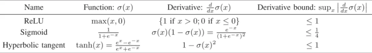
TABLE I
POINT-WISENON-LINEARITIES
be interpreted as a normal to the hyperplane that separates class
ifrom the others. If the last layer is linear the usual choice of learning objective is the hinge loss.
A more common choice for the last layer is the softmax layer:
z=ζ(ˆz) =eˆz/1Teˆz, ˆz=WLzL−1+bL, (17) whereζ(·)is the softmax function andWLandbLare the same as in (16). Note that the exponential is applied element-wise. The elements ofzare in range(0,1)and are often interpreted as “probabilites” associated with the corresponding class la-bels. The decision boundary between classy1 and classy2 cor-responds to the hyperplane{z: (z)y1 = (z)y2}. The softmax layer is usually coupled with categorical cross-entropy training objective.
For the remainder of this work we will take the softmax layer as the last layer of DNN, but note that all results still apply if the linear layer is used.
2) Non-Linear Layers: A non-linear layer is defined as
zl = [ˆzl]
σ = [Wlzl−1+bl]σ, (18) where[ˆzl]
σrepresents the element-wise non-linearity applied to each element ofˆzl ∈RMl, andˆzlrepresents the linear transfor-mation of the layer input:ˆzl=W
lzl−1+bl.Wl ∈RMl×Ml−1 is the weight matrix andbl ∈RMl is the bias vector. The typi-cal non-linearities are the ReLU, the sigmoid and the hyperbolic tangent. They are listed in Table I. The choice of non-linearity
σis usually the same for all the layers in the network.
Note that the non-linear layer in (18) includes the convolu-tional layers which are used in the convoluconvolu-tional neural net-works. In that case the weight matrix is block-cyclic.
3) Pooling Layers: A pooling layer reduces the dimension of intermediate representation and is defined as
zl=Pl(zl−1)zl−1, (19) where Pl(zl−1) is the pooling matrix. The usual choices of pooling are down-sampling, max-pooling and average pooling. We denote by pli(zl−1) thei-th row of Pl(zl−1)and assume that there areMlpooling regionsPi,i= 1, . . . , Ml. In the case of down-samplingpli(zl−1) =ePi(1), wherePi(1)is the first element of the pooling regionPi; in the case of max-pooling
pl
i(zl−1) =ej, wherej = arg maxj∈Pi|(zl−1)j|; and in the case of average poolingpl
i(zl−1) = |Pi1|
j∈Piej. III. THEGEOMETRICALPROPERTIES OFDEEP
NEURALNETWORKS
The classification margin introduced in Section II-A is a function of the decision boundary in the input space. This is visualized in Fig. 2(a). However, a training algorithm usually op-timizes the decision boundary at the network output (Fig. 2(b)),
Fig. 2. Decision boundaries in the input space and in the output space. Plot (a) shows samples of class 1 and 2 and the decision regions produced by a two-layer network projected into the input space. Plot (b) shows the samples transformed by the network and the corresponding decision boundary at the network output.
which does not necessarily imply a large classification margin. In this section we introduce a general approach that allows us to bound the expansion of distances between the network input and its output. In Section IV we use this to establish bounds of the classification margin and the GE bounds that are independent of the network depth or width.
We start by defining the Jacobian matrix (JM) of the DNN
f(x): J(x) = df(x) dx = L l=1 dφl(zl−1) dzl−1 · dφ1(x) dx . (20)
Note that by the properties of the chain rule, the JM is computed as the product of the JMs of the individual network layers,
evaluated at the appropriate values of the layer inputs
x,z1, . . . ,zL−1. We use the JM to establish a relation between a pair of vectors in the input space and the output space.
Theorem 3: For anyx,x∈ Xand a DNNf(·), we have
f(x)−f(x) = 1 0 J(x+t(x−x))dt(x−x) (21) = Jx,x(x−x), (22) where Jx,x = 1 0 J(x+t(x−x))dt (23) is the average Jacobian on the line segment betweenxandx.
Proof: The proof appears in Appendix A. As a direct consequence of Theorem 3 we can bound the distance expansion between x and x at the output of the networkf(·):
Corollary 2: For anyx,x∈ X and a DNNf(·), we have
f(x)−f(x)2 = Jx,x(x−x)2
≤ sup
x∈conv(X)J(x
)
2x−x2. (24) Proof: The proof appears in Appendix B. Note that we have established that Jx,x corresponds to a linear operator that maps the vectorx−xto the vectorf(x)− f(x). This implies that the maximum distance expansion of the network f(x)is bounded by the maximum spectral norm of the network’s JM. Moreover, the JM of f(x)corresponds to the product of JMs of all the layers off(x)as shown in (20). It is possible to calculate the JMs of all the layers defined in Section II-C:
1) Jacobian Matrix of Linear and Softmax Layers: The JM of the linear layer defined in (16) is equal to the weight matrix
dz
dzL−1 =WL. (25) Similarly, in the case of softmax layer defined in (17) the JM is
dz dzL−1 = dz dˆz· dˆz dzL−1 = −ζ(ˆz)ζ(ˆz)T +diag(ζ(ˆz)·WL. (26) Note that−ζ(ˆz)ζ(ˆz)T +diag(ζ(ˆz)corresponds to the JM of the softmax functionζ(ˆz).
2) Jacobian Matrix of Non-Linear Layers: The JM of the non-linear layer (18) can be derived in the same way as the JM of the softmax layer. We first define the JM of the point-wise non-linearity, which is a diagonal matrix4
dzl dzˆl ii =dσ (ˆzl) i d(ˆzl) i , i= 1, . . . , Ml. (27) The derivatives associated with various non-linearities are pro-vided in Table I. The JM of the non-linear layer can be
4Note that in case of ReLU the derivative ofmax(x,0)is not defined for
x= 0, and we need to use subderivatives (or subgradients) to define the JM. We avoid this technical complication and simply take the derivative ofmax(x,0)to be 0 whenx= 0. Note that this does not change the results in any way because the subset ofXfor which the derivatives are not defined has zero measure.
expressed as
dzl
dˆzl−1 =
dzl
dˆzl ·Wl. (28) 3) Jacobian Matrix of Pooling Layers: The pooling operator defined in (19) is linear or a piece-wise linear operator. The corresponding JM is therefore also linear or piece-wise linear and is equal to:
Pl(zl−1). (29)
The following Lemma collects the bounds on the spectral norm of the JMs for all the layers defined in Section II-C.
Lemma 1: The following statements hold:
(1) The spectral norm of JMs of the linear layer in (16), the softmax layer in (17) and non-linear layer in (18) with the ReLU, Sigmoid or Hyperbolic tangent non-linearities is upper bounded by dzl dˆzl−1 2 ≤ Wl2 ≤ WlF. (30) (2) Assume that the pooling regions of the down-sampling, max-pooling and average pooling operators are non-overlapping. Then the spectral norm of their JMs can be upper bounded by ddˆzzl−l1 2 ≤ 1. (31)
Proof: The proof appears in Appendix C. Lemma 1 shows that the spectral norms of all layers can be bounded in terms of their weight matrices. As a consequence, the spectral norm of the JM is bounded by the product of the spectral norms of the weight matrices. We leverage this facts to provide GE bounds in the next section.
We also briefly explore a relationship between the Jaco-bian matrix and the Fisher information matrix. To simplify the derivations we assumeM = 1,N = 1, x=x+θn and
n∼ N(0,1), where θ is the model parameter and x is de-terministic. The Fisher informationF(θ)measures how much information about the parameterθis contained in the random variabley=f(x), wherefrepresents a DNN. In this particular case the Fisher information is given as
F(θ) = En dlogf(x) dθ 2 = En dlogf(x) df(x) df(x) dx dx θ 2 = En dlogf(x) df(x) J(x )n2 . (32) In our setup the parameterθcan be interpreted as a magnitude of the input perturbation. It is clear from (32) that a small norm of the Jacobian matrix leads to a small Fisher information, which indicates that the distribution ofyis not very informative about the parametersθ. By ensuring that the norm of the Jacobian is small we then naturally endow the network with robustness against perturbations of the input.
IV. GENERALIZATIONERROR OF ADEEPNEURAL
NETWORKCLASSIFIER
In this section we provide the classification margin bounds for DNN classifiers that allow us to bound the GE. We follow the common practice and assume that the networks are trained by a loss that promotes separation of different classes at the network output, e.g. categorical cross entropy loss or the hinge loss. In other words, the training aims at maximizing the score of each training sample, where the score is defined as follows.
Definition 3 (Score): Take score of a training sample si= (xi, yi) o(si) = min j=yi √ 2(δyi−δj) Tf(x i), (33) whereδi ∈RNYis the Kronecker delta vector with(δi)i= 1.
Recall the definition of the classifier g(x)in (14) and note that the decision boundary between classi and classj in the feature spaceZ is given by the hyperplane{z: (z)i= (zj)}. A positive score indicates that at the network output, classes are separated by a margin that corresponds to the score. However, a large scoreo(si)does not necessarily imply a large classification marginγd(si). Theorem 4 provides classification margin bounds expressed as a function of the score and the properties of the network.
Theorem 4: Assume that a DNN classifierg(x), as defined in (14), classifies a training samplexiwith the scoreo(si)>0. Then the classification margin can be bounded as
γd(si)≥ o(si) supx:x−xi2≤γd(si)J(x)2 γ1d(si) (34) ≥ o(si) supx∈conv(X)J(x)2 γ2d(si) (35) ≥ o(si) Wl∈WWl2 γ3d(si) (36) ≥ o(si) Wl∈WWlF γ4d(si), (37)
whereWis the set of all weight matrices off(x).
Proof: The proof appears in Appendix D. Given the bounds of the classification margin we can special-ize Corollary 1 to DNN classifiers.
Corollary 3: Assume that X is a (subset of) CM regular
k-dimensional manifold, whereN(X;d, ρ)≤(CM ρ )
k. Assume also that DNN classifier g(x)achieves a lower bound to the classification marginγd
b(si)> γbforb∈ {1,2,3,4},∀si∈Sm and take(g(xi), yi)to be the 0-1 loss. Then for anyδ >0, with probability at least1−δ, GE(g)≤ log(2)·NY·2k+1·(C M)k γk bm + 2 log(1/δ) m . (38) Proof: The proof follows from Theorems 1, 2 and 4. Corollary 3 suggests that the GE will be bounded by
C√1 mγ−
k /2, where C=log(2)·N
Y2k+1(CM)k, provided
that the classification margin bounds satisfy γbd(si)> γ for someb∈ {1,2,3,4},∀si∈Sm.
We now leverage the classification margin bounds in Theo-rem 4 to construct constraint setsWb ={Wl∈ W :γbd(si)>
γ∀si},b∈1,2,3,4such thatW ∈ Wb ensures that the GE is bounded byC√1 mγ− k /2. Using (34)-(37) we obtain W1 = Wl∈ W : sup x:x−xi2≤γd(s i) J(x)2 < γ·o(si) ∀si= (xi, yi) , (39) W2 = Wl∈ W : sup x∈conv(X) J(x)2 < γ·o(si) ∀si= (xi, yi) , (40) W3 = Wl∈ W : Wl∈W Wl2 < γ·o(si) ∀si= (xi, yi) , (41) W4 = Wl∈ W : Wl∈W WlF < γ·o(si) ∀si= (xi, yi) . (42) Note that while we want to maximize the scoreo(si), we also need to constrain the network’s Jacobian matrixJ(x)(following
W1 andW2) or the weight matricesWl ∈ W (followingW3 andW4). This stands in line with the common training ratio-nale of DNN in which we do not only aim at maximizing the score of the training samples to ensure a correct classification of the training set, but also have a regularization that constrains the network parameters, where this combination eventually leads to a lower GE. The constraint sets in (39)–(42) impose different regularization techniques:
r
The termsupx:x−xi2≤γd(si)J(x)2< γ·o(si)in (39) considers only the supremum of the spectral norm of the Jacobian matrix evaluated at the points withinNi={x:
x−xi2 ≤γd(si)}, where γd(si) is the classification margin of training samplesi (see Definition 2). We can not compute the marginγd(s
i), but can still obtain a ra-tionale for regularization: as long as the spectral norm of the Jacobian matrix is bounded in the neighbourhood of a training sample xi given by Ni we will have the GE guarantees.
r
The constraint on the Jacobian matrix supx∈conv(X)J(x)2 < γ·o(si) in (40) is more restrictive as it re-quires bounded spectral norm for all samples x in the convex hull of the input spaceX.
r
The constraints in (41) and (42) are of similar form, Wl∈WWl2 < γ·o(si) and
Wl∈WWlF < γ·
o(si), respectively. Note that the weight decay, which aims at bounding the Frobenious norms of the weight matrices
might be used to satisfy the constrains in (42). However, note also that the bound based on the spectral norm in (41) is tighter than one based on the Frobenious norm in (42). For example, takeWl ∈ W to have orthonormal rows and be of dimensionM×M. Then the constraint in (41), which is based on the spectral norm, is of the form 1< γo(si)and the constraint in (42), which is based on the Frobenious norm, is ML /2 < γo(si). In the former case we have a constraint on the score, which is inde-pendent of the network width or depth. In the latter the constraint on the output score is exponential in network depth and polynomial in network width. The difference is that the Frobenious norm does not take into account the correlation (angles) between the rows of the weight matrix
Wl, while the spectral norm does. Therefore, the bound based on the Frobenious norm corresponds to the worst case when all the rows of Wl are aligned. In that case
WlF =Wl2 =
√
M. On the other hand, if the rows ofWlare orthonormalWlF =
√
M, butWl2 = 1. Remark 1: To put results into perspective we compare our GE bounds to the GE bounds based on the Rademacher com-plexity in [33], which hold for DNNs with ReLUs. The work in [33] shows that if W ∈ WF = Wi ∈ W: L i=1 WiF < CF (43)
and the energy of training samples is bounded then:
GE(g) √1 m2
L−1C
F . (44)
Although the bounds (38) and (44) are not directly comparable, since the bounds based on the robustness framework rely on an underlying assumption on the data (covering number), there is still a remarkable difference between them. The behaviour in (44) suggests that the GE grows exponentially with the network depth even if the product of the Frobenious norms of all the weight matrices is fixed, which is due to the term 2L. The bound in (34) and the constraint sets in (39)–(42), on the other hand, imply that the GE does not increase with the number of layers provided that the spectral/Frobenious norms of the weight matrices are bounded. Moreover, if we take the DNN to have weight matrices with orthonormal rows then the GE behaves as
1 √
m(CM)
k /2(assumingo(s
i)≥1, i= 1, . . . , m), and therefore relies only on the complexity of the underlying data manifold and not on the network depth. This provides a possible answer to the open question of [33] that depth independent capacity control is possible in DNNs with ReLUs.
Remark 2: An important value of our bounds is that they provide an additional explanation to the success of state-of-the-art DNN training techniques such as batch normalization [23] and eight normalization [24].
Weight normalized DNNs have weight matrices with normal-ized rows, i.e.
Wl =diag( ˆWTl Wˆl)−1Wˆl, (45)
where diag(·) denotes the diagonal part of the matrix. While the main motivation for this method is a faster training, the au-thors also show empirically that such networks achieve good generalization. Note that for row-normalized weight matrices
WlF =
√
Ml and therefore the bounds based on the Frobe-nious norm can not explain the good generalization of such networks as adding layers or making Wl larger will lead to a larger GE bound. However, our bound in (34) and the con-straint sets in (39)–(41) show that a small Frobenious norm of the weight matrices is not crucial for a small GE. A supporting experiment is presented in Section VI-A2.
We also note that batch normalization also leads to row-normalized weight matrices in DNNs with ReLUs:5
Theorem 5: Assume that the non-linear layers of a DNN with ReLUs are batch normalized as:
zl+1 = [N{zl
i}mi=1,Wl
ˆ zl]
σ, ˆzl =Wlzl, (46) whereσdenotes the ReLU non-linearity and
N({zi}mi=1,W) =diag m i=1 WzizTi WT −1 2 (47) is the normalization matrix. Then all the weight matrices are row normalized. The exception is the weight matrix of the last layer, which is of the formN({zLi−1}mi=1,WL)WL.
Proof: The proof appears in Appendix E. A. Jacobian Regularizer
The constraint set (39) suggests that we can regularize the DNN by bounding the norm of the network’s JM for the inputs close toxi. Therefore, we propose to penalize the norm of the network’s JM evaluated at each training samplexi,
RJ(W) = 1 m m i=1 J(xi)22. (48)
The implementation of such regularizer requires computation of its gradients or subgradients. In this case the computation of the subgradient of the spectral norm requires the calcula-tion of a SVD decomposicalcula-tion [44], which makes the proposed regularizer inefficient. To circumvent this, we propose a surro-gate regularizer based on the Frobenious norm of the Jacobian matrix: RF(W) = 1 m m i=1 J(xi)2F. (49)
Note that the Frobenious norm and the spectral norm are related as follows:1/rank(J(xi))J(xi)2F ≤ J(xi)22 ≤ J(xi)2F, which justifies using the surrogate regularizer. We will refer to
RF(W)as the Jacobian regularizer.
5To simplify the derivation we omit the bias vectors and therefore also the
centering applied by the batch normalization. This does not affect the generality of the result. We also follow [43] and omit the batch normalization scaling, as it can be included into the weight matrix of the layer following the batch normalization. We also omit the regularization term and assume that the matrices are invertible.
1) Computation of Gradients and Efficient Implementation: Note that thek-th row ofJ(xi)corresponds to the gradient of (f(x))k with respect to the inputxevaluated atxi. It is denoted bygk(xi) = d(fd(xx))k|x=xi. Now we can write
RF(W) = 1 m m i=1 M k=1 gk(xi)gk(xi)T. (50) As the regularizer will be minimized by a gradient descent algorithm we need to compute its gradient with respect to the DNN parameters. First, we expressgk(xi)as
gk(xi) =gkl(xi)WlJl−1(xi) (51) wheregl
k(xi) =d(fdˆ(zxl))k|x=xi is the gradient of(f(x))k with respect tozˆlevaluated at the inputxiandJl−1(xi) =dz
l−1 dx |x=xi is the JM ofl−1-th layer outputzl−1 evaluated at the inputxi. The gradient ofgk(xi)gk(xi)T with respect toWlis then given as [45] ∇Wl gk(xi)gk(xi)T = 2gl k(xi)Tglk(xi)WlJl−1(xi). The computation of the gradient of the regularizer at layer l
requires the computation of gradients gkl(xi), k= 1, . . . , M,
i= 1, . . . , m and the computation of the Jacobian matrices
Jl−1(x
i),i= 1, . . . , m. The computation of the gradient of a typical loss used for training DNN usually involves a computa-tion ofmgradients with computational complexity similar to the computational complexity ofgl
k(xi). Therefore, the computa-tion of gradients required for an implementacomputa-tion of the Jacobian regularizer can be very expensive.
To avoid excessive computational complexity we propose a simplified version of the regularizer (49), which we name per-layer Jacobian regularizer. The per-per-layer Jacobian regularizer at layerlis defined as RlF(Wl) = 1 m m i=1 ˜ gl−1 π(i)(xi)(˜gπ(i)l−1(xi))T, (52) whereg˜πl−(i)1(xi) = d(f(x))π(i) dzl−1 |x=xi, andπ(i)∈ {1, . . . , M}is a random index. Compared to (49) we have made two simpli-fications. First, we assumed that input of layerlis fixed. This way we do not need to compute the JMJl−1(x
i)between the output of the layerl−1 and the input. Second, by choosing only one indexπ(i)per training sample we have to compute only one additional gradient per training sample. This signifi-cantly reduces the computational complexity. The gradient of ˜
gl−1
π(i)(xi)(˜glπ−(i)1(xi))T is simply
∇Wl ˜ gl−1 π(i)(xi)(˜g l−1 π(i)(xi))T = 2gl π(i)(xi)Tglπ(i)(xi)Wl. We demonstrate the effectiveness of this regularizers in Section VI.
V. DISCUSSION
In the preceding sections we analysed the standard feed-forward DNNs and their classification margin measured in the Euclidean norm. We now briefly discuss how our results extend to other DNN architectures and different margin metrics.
A. Beyond Feed Forward DNN
There are various DNN architectures such as Residual Net-works (ResNets) [4], [46], Recurrent Neural NetNet-works (RNNs) and Long Short-Term Memory (LSTM) networks [47], and Auto-encoders [48] that are used frequently in practice. It turns out that our analysis—which is based on the network’s JM— can also be easily extended to such DNN architectures. In fact, the proposed framework encompasses all DNN architectures for which the JM can be computed. Below we compute the JM of a ResNet.
The ResNets introduce shortcut connection between layers. In particular, letφ(·, θl)denote a concatenation of several non-linear layers (see (18)). Thel-th block of a Residual Network is then given as
zl=zl−1+φ(zl−1, θ
l). (53)
We denote byJl(zl−1)the JM ofφ(zl−1, θl). Then the JM of thel-th block is
dzl
dzl−1 =I+Jl(z
l−1), (54)
and the JM of a ResNet is of the form
JS M(zL−1)· I+ L l=1 Jl(zl−1) l−1 i=1 (I+Jl−i(zl−2)) , (55) where JS M(zL−1) denotes the JM of the soft-max layer. In particular, the right element of the product in (55) can be expanded as I+J1(x) +J2(z1) +J2(z1)J1(x) +J3(z2) +J3(z2)J2(z1)J1(x) +J3(z2)J2(x) +J3(x)J1(x) +. . .
This is a sum of JMs of all the possible sub-networks of a ResNet. In particular, there areLelements of the sum consisting only of one 1-layer sub-networks and there is only one element of the sum consisting ofL-layer sub-network. This observation is consistent with the claims in [49], which states that ResNets resemble an ensemble of relatively shallow networks.
B. Beyond the Euclidean Metric
Moreover, we can also consider the geodesic distance on a manifold as a measure for margin instead of the Euclidean distance. The geodesic distance can be more appropriate than the Euclidean distance since it is a natural metric on the man-ifold. Moreover, the covering number of the manifold X may be smaller if we use the covering based on the geodesic met-ric balls, which will lead to tighter GE bounds. We outline the approach below.
Assume that X is a Riemannian manifold and x,x∈ X. Take a continuous, piecewise continuously differentiable curve
c(t),t= [0,1]such thatc(0) =x,c(1) =xandc(t)∈ X ∀t∈
[0,1]. The set of all such curvesc(·)is denoted byC. Then the geodesic distance betweenxandxis defined as
dG(x,x) = inf c(t)∈C 1 0 dc(t) dt 2 dt . (56) Similarly as in Section III, we can show that the JM of DNN is central to bounding the distance expansion between the signals at the DNN input and the signals at the DNN output.
Theorem 6: Take x,x∈ X, where X is the Riemmanian manifold and takec(t),t= [0,1]to be a continuous, piecewise continuously differentiable curve connectingxandxsuch that
dG(x,x) = 1 0 dc(t)dt 2dt. Then f(x)−f(x)2 ≤ sup t∈[0,1] J(c(t))2dG(x,x) (57) Proof: The proof appears in Appendix F. Note that we have established a relationship between the Euclidean distance of two points in the output space and the corresponding geodesic distance in the input space. This is important because it implies that promoting a large Euclidean distance between points can lead to a large geodesic distance between the points in the input space. Moreover, the ratio be-tweenf(x)−f(x)2anddG(x,x)is upper bounded by the maximum value of the spectral norm of the network’s JM eval-uated on the linec(t). This result is analogous to the results of Theorem 3 and Corollary 2. It also implies that regularizing the network’s JM as proposed in Section IV is beneficial also in the case when the classification margin is not measured in the Euclidean metric.
Finally, note that in practice the training data may not be balanced. The provided GE bounds are still valid in such cases. However, the classification error may not the best measure of performance in such cases as it is dominated by the classification error of the class with the highest prior probability. Therefore, alternative performance measures need to be considered. We leave a detailed study of training DNN with unbalanced training sets for possible future work.
VI. EXPERIMENTS
We now validate the theory with a series of experiments on the MNIST [50], CIFAR-10 [51], LaRED [52] and ImageNet (ILSVRC2012) [53] datasets. The Jacobian regularizer is ap-plied to various DNN architectures such as DNN with fully connected layers, convolutional DNN and ResNet [4]. We use the ReLUs in all considered DNNs as this is currently the most popular non-linearity.
A. Fully Connected DNN
In this section we compare the performance of fully con-nected DNNs regularized with Jacobian Regularization or with the weight decay. Then we analyse the behaviour of the JM of a fully connected DNNs of various depth and width.
1) Comparison of Jacobian Regularization and Weight De-cay: First, we compare standard DNN with fully connected
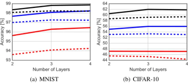
Fig. 3. Classification accuracy of DNNs trained with the jacobian regular-ization (solid lines) and the weight decay (dashed lines). Different numbers of training samples are used: 5000 (red), 20000 (blue) and 50000 (black).
layers trained with the weight decay and the Jacobian regular-ization (49) on the MNIST and CIFAR-10 datasets. Different number of training samples are used (5000, 20000, 50000). We consider DNNs with 2, 3 and 4 fully connected layers where all layers, except the last one, have dimension equal to the input signal dimension, which is 784 in case of MNIST and 3072 in case of CIFAR-10. The last layer is always the softmax layer and the objective is the CEE loss. The networks were trained using the stochastic gradient descent (SGD) with momentum, which was set to 0.9. Batch size was set to 128 and learning rate was set to 0.01 and reduced by factor 10 after every 40 epochs. The networks were trained for 120 epochs in total. The weight decay and the Jacobian regularization factors were chosen on a separate validation set. The experiments were repeated with the same regularization parameters on 5 random draws of training sets and weight matrix initializations. Classification accuracies averaged over different experimental runs are shown in Fig. 3. We observe that the proposed Jacobian regularization always outperforms the weight decay. This validates our theoretical re-sults in Section IV, which predict that the Jacobian matrix is crucial for the control of (the bound to) the GE. Interestingly, in the case of MNIST, a 4 layer DNN trained with 20000 training samples and Jacobian regularization (solid blue line if Fig. 3(a)) performs on par with DNN trained with 50000 training samples and weight decay (dashed black line Fig. 3(a)), which means that the Jacobian regularization can lead to the same performance with significantly less training samples.
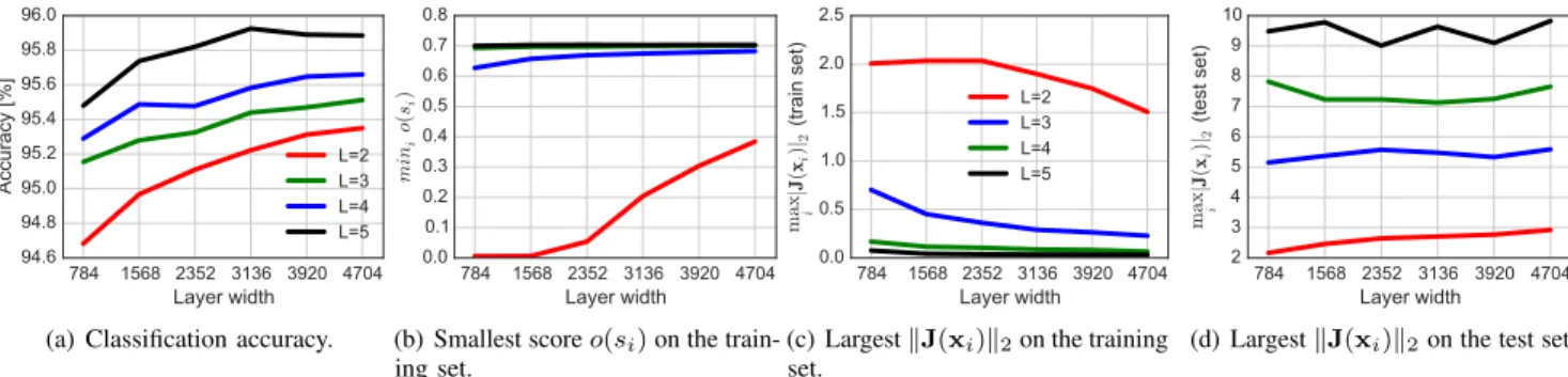
2) Analysis of Weight Normalized Deep Neural Networks: Next, we explore weight normalized DNNs, which are described in Section IV. We use the MNIST dataset and train DNNs with a different number of fully connected layers (L= 2,3,4,5) and different sizes of weight matrices (Ml = 784,2·784,3· 784,4·784,5·784,6·784, l= 1, . . . , L−1). The last layer is always the softmax layer and the objective is the CCE loss. The networks were trained using the stochastic gradient descent (SGD) with momentum, which was set to 0.9. Batch size was set to 128 and learning rate was set to 0.1 and reduced by fac-tor 10 after every 40 epochs. The networks were trained for 120 epochs in total. All experiments are repeated 5 times with different random draws of a training set and different random weight initializations. We did not employ any additional regu-larization as our goal here is to explore the effects of the weight
Fig. 4. Weight normalized DNN withL= 2,3,4,5layers and different sizes of weight matrices (layer width). Plot (a) shows classification accuracy, plot (b) shows the smallest score of training samples, plot (c) shows the largest spectral norm of the network’s JM evaluated on the training set and plot (d) shows the largest spectral norm of the network’s JM evaluated on the testing set.
normalization on the DNN behaviour. We always use 5000 train-ing samples.
The classification accuracies are shown in Fig. 4(a) and the smallest classification score obtained on the training set is shown in Fig. 4(b). We have observed for all configurations that the training accuracies were 100% (only exception is the caseL= 2,Ml = 784where the training accuracy was 99.6%). Therefore, the (testing set) classification accuracies increasing with the network depth and the weight matrix size directly im-ply that the GE is smaller for deeper and wider DNNs. Note also that the score increases with the network depth and width. This is most obvious for the 2 and 3 layer DNNs, whereas for the 3 and 4 layer DNNs the score is close to√2for all network widths.
Since the DNNs are weight normalized, the Frobenious norms of the weight matrices are equal to the square root of the weight matrix dimension, and the product of Frobenious norms of the weight matrices grows with the network depth and the weight matrix size. The increase of score with the network depth and network width does not offset the product of Frobenious norms, and clearly, the bound in (38) based on the margin bound in (37) and the bound in (44), which leverage the Frobenious norms of the weight matrices, predict that the GE will increase with the network depth and weight matrix size in this scenario. Therefore, the experiment indicates that these bounds are too pessimistic.
We have also inspected the spectral norms of the weight matrices of the trained networks. In all cases the spectral norms were greater than one. We can argue that the bound in (38) based on the margin bound in (36) predicts that the GE will increase with network depth, as the product of the spectral norms grows with the network depth in a similar way than in previous paragraph. We note however, that the spectral norms of the weight matrices are much smaller than the Frobenious norms of the weight matrices.
Finally, we look for a possible explanation for the success of the weight normalization in the bounds in (38) based on the margin bounds in (34) and (35), which are a function on the JM. The largest value of the spectral norm of the network’s JM evaluated on the training set is shown in Fig. 4(c) and the largest value of the spectral norm of the network’s JM evaluated on the testing set is shown in Fig. 4(d).
We can observe an interesting phenomena. The maximum value of the JM’s spectral norm on the training set decreases with the network depth and width. On the other hand, the max-imum value of the JM’s spectral norm on the testing set in-creases with network depth (and slightly with network width). From the perspective of the constraint sets in (39) and (40) we note that in the case of the latter we have to take into account the worst case spectral norm of the JM for inputs in conv(X). The maximum value of the spectral norm on the testing set indicates that this value increases with the network depth and implies that the bound based on (35) is still loose. On the other hand, the bound in (34) implies that we have to consider the JM in the neighbourhood of the training samples. As an approxi-mation, we can take the spectral norms of the JMs evaluated at the training set. As it is shown in Fig. 4(c) this values decrease with the network depth and width. We argue that this provides a reasonable explanation for the good generalization of deeper and wider weight normalized DNNs.
B. Convolutional DNN
In this section we compare the performance of convolutional DNNs regularized with the Jacobian regularizer or with the weight decay. We also show that Jacobian Regularization can be applied to batch normalized DNNs. We will use the standard MNIST and CIFAR-10 dataset and the LaRED dataset which is briefly described below.
The LaRED dataset contains depth images of 81 distinct hand gestures performed by 10 subjects with approximately 300 im-ages of each gesture per subject. We extracted the depth imim-ages of the hands using the masks provided in [52] and resized the images to32×32. The images of the first 6 subjects were used to create non-overlapping training and testing sets. In addition we also constructed a testing set composed from the images of the last 4 subjects in the dataset in order to test generalization across different subjects. The goal is classification of gestures based on the depth image.
1) Comparison of Jacobian Regularization and Weight De-cay: We use a 4 layer convolutional DNN with the following architecture: (32,5,5)-conv, (2,2)-max-pool, (32,5,5)-conv, (2,2)-max-pool followed by a softmax layer, where (k, u, v)-conv denotes the convolutional layer withk filters of size
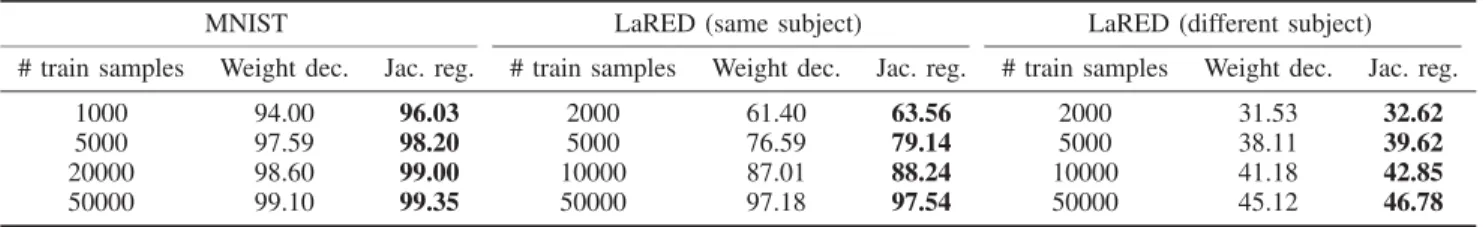
TABLE II
CLASSIFICATIONACC.[%]OFCONVOLUTIONALDNNONMINSTANDLARED
TABLE III
CLASSIFICATIONACC.[%]OFCONVOLUTIONALDNNONCIFAR-10
u×v and(p, p)-max-pool denotes max-pooling with pooling regions of sizep×p. The training procedure follows the one described in the previous paragraphs. The results are reported in Table II.
We observe that training with the Jacobian regularization outperforms the weight decay in all cases. This is most obvious at smaller training set sizes. For example, on the MNIST dataset, the DNN trained using 1000 training samples and regularized with the weight decay achieves classification accuracy of 94% and the DNN trained with the Jacobian regularization achieves classification accuracy of 96.3%.
Similarly, on the LaRED dataset the Jacobian regularization outperforms the weight decay with the difference most obvious at the smallest number of training samples. Note also that the generalization of the network to the subjects outside the training set is not very good; i.e., using 50000 training samples the classi-fication accuracy on the testing set containing the same subjects is higher than 97% whereas the classification accuracy on the testing set containing different subjects is only 46%. Neverthe-less, the Jacobian regularization outperforms the weight decay also on this testing set by a small margin.
2) Batch Normalization and Jacobian Regularization: Now we show that the Jacobian regularization (49) can also be ap-plied to a batch normalized DNN. Note that we have shown in Section IV that the batch normalization has an effect of normalizing the rows of the weight matrices.
We us the CIFAR-10 dataset and use the All-convolutional-DNN proposed in [54] (All-CNN-C) with 9 convolutional layers, an average pooling layer and a softmax layer. All the convolutional layers are batch normalized and the softmax layer is weight normalized. The networks were trained using the stochastic gradient descent (SGD) with momentum, which was set to 0.9. Batch size was set to 64 and the learning rate was set to 0.1 and reduced by a factor 10 after every 25 epochs. The networks were trained for 75 epochs in total. The classification accuracy results are presented in Table III for different sizes of training sets (2500, 10000, 50000).
We can observe that the Jacobian regularization also leads to a smaller GE in this case.
TABLE IV
CLASSIFICATIONACC.[%]OFRESNETCIFAR-10
C. Residual Networks
Now we demonstrate that the Jacobian regularizer is also effective when applied to ResNets. We use the CIFAR-10 and ImageNet datasets. We use the per-layer Jacobian regularization (52) for experiments in this section.
1) CIFAR-10: The Wide ResNet architecture proposed in [35], which follows [46], but proposes wider and shallower networks which leads to the same or better performance than deeper and thinner networks is used here. In particular, we use the ResNet with 22 layers of width 5.
We follow the data normalization process of [35]. We also follow the training procedure of [35] except for the learning rate and use the learning rate sequence: (0.01, 5), (0.05, 20), (0.005, 40), (0.0005, 40), (0.00005, 20), where the first number in parenthesis corresponds to the learning rate and the second number corresponds to the number of epochs. We train ResNet on small training sets (2500 and 10000 training samples) without augmentation and on the full training set with the data augmen-tation as in [35]. The regularization factor were set to 1 and 0.1 for the smaller training sets (2500 and 10000) and the full augmented training set, respectively.
The results are presented in Table IV. In all cases the ResNet with Jacobian regularization outperforms the standard ResNet. The effect of regularization is the strongest with the smaller number of training samples, as expected.
2) ImageNet: We use the 18 layer ResNet [4] with identity connection [46]. The training procedure follows [4] with the learning rate sequence: (0.1, 30), (0.01, 30), (0.001, 30). The Jacobian regularization factor is set to 1.
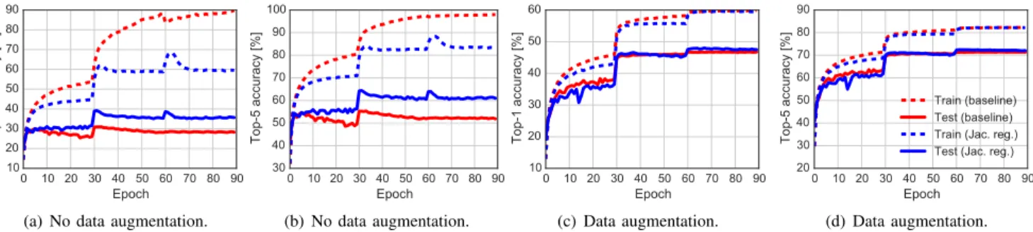
The images in the dataset are resized to128×128. We run an experiment without data augmentation and with data augmenta-tion following [1], which includes random cropping of images of size112×112from the original image and color augmenta-tion. The classification accuracies during training are shown in Fig. 5 and the final results are reported in Table V.
We first focus on training without data augmentation. The ResNet trained using the Jacobian regularization has a much smaller GE (23.83%) compared to the baseline ResNet