A Hybrid AANN-KPCA Approach to Sensor Data Validation
REZA SHARIFI, REZA LANGARI Department of Mechanical Engineering
College Station TX-77843 USA
[email protected], [email protected],
http://www.mengr.tamu.edu/People/facultyinfo.asp?LastName=langari
Abstract: - In this paper two common methods for nonlinear principal component analysis are com-pared. These two methods are Auto-associative Neural Network (AANN) and Kernel PCA (KPCA). The performance of these methods in sensor data validation are discussed, finally a methodology which takes advantage of both of these methods is presented. The result is a unique approach to nonlinear component mapping of a given set of data obtained from a nonlinear quasi-static system. This method is finally compared with AANN and KPCA for sensor data validation and shows a better performance in terms of predicting/reconstructing the missing or corrupted channels of data.
Key-Words: -Nonlinear PCA, Kernel PCA, Sensor Fault Detection, Auto associative Neural Network
1.
Introduction
Principal component analysis (PCA) is a mathematical technique that is used for compres-sion of linearly correlated data. Introduced by Pearson [1] in 1901 and individually developed by Hotteling [2] in 1933, this technique finds the di-rections with maximum variance in n-dimensional set of data, and transforms the data into new coor-dinate which is a set of “n” orthonormal vector that have the maximum variance. When trans-formed, the directions with least variance which are called as noise directions are eliminated and the remaining dimensions contain the maximum information of original data with minimum possi-ble dimension.
Because of the capability of compression of data, this PCA is very common in data processing methods. It is also widely been used for noise fil-tering and data validation in linear systems. PCA based data-driven fault diagnosis method, which only depends on the input and output data of the monitored process, have found broad applications since 1990’s, especially in process industry [3-6]. The core basis of all these methods is that the data obtained from sensors is initially compressed and subsequently uncompressed or de-mapped into the original set of data. Since PCA is a linear tech-nique its performance in sensor fault diagnosis is
acceptable as long as we have adequate co-linearity between different sensor readings. But, most real systems do not satisfy this property. Therefore, we need to find an alternative nonlinear method.
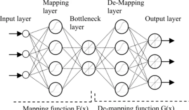
Nonlinear principal component analysis was introduced by Kramer in 1991 [7]. He used a spe-cific architecture of neural network to train a unity network. The architecture of an Autoassociative neural network (AANN) is shown in Figure1. AANN is a five layer feed forward neural network where the second and forth layers incorporate nonlinear transfer functions while the third layer as well as the output layer have linear transfer function. In this architecture the third layer has the least number of neurons. In principle this network provides and identity map [7]; i.e. output of the network is the same as its input. A key element in the operation of the network is the fact that it finds the nonlinear correlation between different chan-nels of input.
This is accomplished mainly via the so called bottleneck layer which has fewer nodes than the input and output layers. This layer in effect acts like a feature detector. In other word the original data are nonlinearly mapped into fewer dimen-sions than their original form and subsequently de-mapped to their original form. Therefore we can
expect that the data in the reduced dimension sec-tion act as a nonlinear principal component of the original data. The nonlinear relation for the first principal component is as follows.
∑
∑
= > < = > < σ = = n 1 j j 1 ij p 1 i 2 i 1 1 1 F(x) w ( w x ) Pc (1)where are the elements of the weight matrix of the kth layer in the neural network, x is the vector of inputs with dimension of n, p is the number of neurons in the mapping layer and σ is the activation function of the relevant neuron.
> − <k 1
ij w
Figure 1 - Architecture of Autoassociative Neural Network
Several successful applications of AANN in sensor fault diagnosis have been presented since its birth in 1991. Hines, et al used AANN for sen-sor data validation in nuclear power plant [8]. Mattern, et al Applied this method for turbofan engine [9]. Antory, et al. have used this method for industrial process monitoring [10]. In spite of these, there are several difficulties in using AANN for sensor data validation. First of all, like any other neural networks, we need to find the mini-mum number of adjustable parameters in the net-work that can model our function within a certain error. This job is much more challenging in AANN because we have a large network of five layers. Another problem is to find the best archi-tecture of the neural network. Kramer [7] in his introductory paper on AANN has presented some upper limits for the number of neurons in each layer but in reviewing the application of AANNs in different areas, it is evident that the best archi-tecture usually has far less parameters (neurons)
than the proposed “upper limit” by Kramer. [11-13]
This problem is even more considerable when it comes to the number of neurons in bottleneck. In fact, the number of neurons in bottleneck is the number of principal components and can be ex-pressed as the number of independent variables in the observed parameters. Therefore selecting more neurons for the bottleneck than the number of in-dependent parameters questions the rationality of using principal components. In next part a method for finding the size of bottleneck in AANN is pre-sented.
The second problem is that there is no spe-cific training methodology for AANN. All of the studied papers in the literature have used the regu-lar backpropagation algorithm for training. Having a neural network with 5 layers at least two of which have nonlinear transfer functions makes it very difficult to train network. In fact training the network is an optimization problem with a very complicated and nonlinear objective function. With the real observed variables which usually are noisy, objective functions have multiple local minimums around the minimum. This problem limits the application of AANNs for sensor fault diagnosis to a very narrow category of systems which have simple forms of nonlinear correlation.
Mapping function F(x) De-mapping function G(x) Bottleneck layer Mapping layer De-Mapping layer Output layer Input layer
The most important problem with AANNs is that there is no unique solution for the trained network. In other words each time we train the network with different initial conditions, we get different final weights for the network. Therefore we have different sets of nonlinear principal com-ponents. Apparently some of these mappings have better performance of fault detection than others. Therefore, the immediate question is that how should we train the network to perform well in sensor fault diagnosis. This problem is also ad-dressed in this paper in the next section.
2.
Kernel Principal Component Analysis
Method of Kernel Principal Component Analysis (KPCA) is introduced by Scholkopf et al [14] in 1998. The simplicity of method and its ra-tional mathematical base has made this method very favorable. Numerous applications of this method have been presented Sine its publication,
especially in pattern recognition [15-20], but few of them are in sensor data validation [21],[22].
In this method, Instead of solving principal components in original space, x, we find the prin-cipal component of a nonlinear transformation of this space where usually have higher dimension than x and even can have infinite di-mension. But as we will see, we never need to do any calculation in this high dimensional space.
) (x
Φ Φ(x)
Assuming the mapping data are centered i.e. , we can write the covariance matrix:
∑
Φ = M (xk) 0∑
= Φ Φ = M 1 j T j j) ( ) ( M 1 C x x (2)where M is number of observed samples. In order to find the principal values we need to find the ei-genvalues and eigenvectors of covariance matrix:
CV V =
λ (3)
Knowing the fact that all solutions of V lie in the span of [10]. We can write the vector V as follow: ) ( ),..., (x1 Φ xM Φ ) ) ( ( 1
∑
= Φ = M i i i V α x (4) Solving this equation lead to the following Eigenvalue problemα α K
Mλ = (5) where K is called kernel matrix and is defined as following )) ( ) ( ( : i j ij K = Φ x ⋅Φ x (6)
and is the vector of α αi which are coeffi-cients of eigenvectors used in equation 4.
After normalizing the eigenvectors, in order to find the principal components we have to project the data into the normalized eigenvectors. There-fore, the kth principal value is
∑
= Φ ⋅ Φ = Φ ⋅ = M i i k i k k V Pc 1 )) ( ) ( ( )) ( ( x α x x (7)One interesting characteristic of Kernel PCA is that we never need to calculate the nonlinear map-pingΦ. In fact, we are always dealing with the dot product of two mapping function. Therefore, In-stead of selecting functionΦ, we can select a ker-nel function in the following form
) ( ) ( ) , ( i j i j k x x =Φ x ⋅Φ x (8) R R k: n → In other word, the dimension of nonlinear transfer function can be infinitely large because we never actually work in that space.
Several kernel functions are discussed by Boser et al. [23] and Vapnic et al. [24], but the most kernel function used in KPCA applications is Radial Basis Function defied as
) 2 exp( ) , ( 2 2 σ y x y x = − − k (9) The proposed method of sensor fault diagno-sis with KPCA is to find the principal components of observed data using a specific kernel function, then, find inverse transform of these principal components back to the original space.
This process, however, has some shortcom-ings. First of all we need to know what is the best kernel function for this and what are the parame-ters of that function for example if we select Ra-dial Basis Function, defined in equation 12, The value of σ is important as well.
Also, size of kernel matrix is square of the number of observed variables. Therefore, with high number of training variables, we have a big kernel matrix and very high volume of calcula-tions.
Another problem is that using KPCA in this form is in fact a “lazy” method in which we are using all of the training data during the online classification of data. Evidently, these types of algorithms take a lot of processing time and mem-ory space and with a high volume of training data this method fails in performance.
3.
Sensor Fault Diagnosis with Kernel
PCA
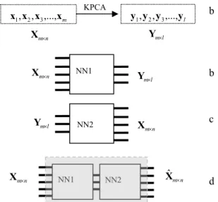
If we find the nonlinear principal components of the data, with KPCA algorithm, we can train a simple network to map the data to the found prin-cipal components. It is also very simple to train another network to reconstruct the original data out of the principal values. Using these two net-works serially net-works like an Autoassociative Neu-ral Network but the difference is that we have a predefined mapping function which is found based on a rational logic. Figure 2 shows this procedure.
Using KPCA can also help in finding the number of independent variables or the number of neurons in the bottleneck layer of AANN, because the number of principal components is actually the number of independent valuables. Therefore, this method can be used as a supporting method for AANN. This procedure is explained in the next section as an example. Another indirect appliance of KPCA is to use the number of principal com-ponents found in this algorithm as the number of neurons in bottleneck layer in AANN. In other word before we apply AANN, we have an insight about the number of independent variables in the training dataset.
Figure 2- Schematic diagram of sensor fault diagnosis using KPCA
Table 1 compares briefly the two methods of AANN and KPCA. Phrases in the shaded table cells are disadvantages of the method
Table 1 Comparison of KPCA and AANN
Kernel Principal component Autoassociative Neural
Net-Analysis work
The algorithm gives the number We have to assume the number
of principal components of principal components
The training is a simple linear The training needs nonlinear
procedure optimization
principal components are
unique Non unique solution
Mapping function is limited to the selected kernel function
Capable of wide category of mapping functions Slow algorithm with large
number of observations No problem with large number of observations
The training data is not needed
Lazy algorithm when trained
4.
Application of Method in a Sample
compare these methods quantita-tivel + = + − = + + = + − = 5 2 1 5 4 2 1 4 3 2 1 3 2 2 1 2 ) (sin ) cos( ) cos( ) sin( e t x e t t x e t t x e t t x
Where are measurements and and
a endent o
da
Problem
In order to
y, a sample problem is solved using AANN and KPCA. In this problem we assume that we have five measurements which are functions of two independent variables. Defined as follows:
⎧x1=t1+t2+e1 ⎪ ⎪ ⎪ ⎩ ⎪⎪ ⎪ ⎨ KPCA m x x x x1, 2, 3,..., n m× X l y y y y1, 2, 3,..., l m× Y n m× X l m× Y n m× X l m× Y n m× X NN1 NN2 NN1 NN2 Xˆm×n b b c d 5 1,...,x x t1 2
t re indep variables. In order to pr vide ta for this problem, 100 random numbers in the range [0,π/2] were generated. Values of e1,...,e5 are nor Gaussian random numbers with the mean of zero and standard deviation defined as follows malized i i =0.05⋅Range(x) σ where
In order to find the best architecture of AANN, 16 different architectures has been tested, and for each one process of training has been done 25 times. The algorithm of training is Backpropa-gation with Levenberg-Marquardt optimization
algorithm. Two category of architecture are in format of 5-J-2-J-5 and 5-J-3-J-5 for the values of J from 4 to 12
Minimum training error is shown in figure 3. As y of net-wor = = ,
After generation of the correct values of all 5 sen-ou see for values of J>7 the amsen-ount of train-ing error does not change considerably with fur-ther increasing of the number of neurons. There-fore, the number of neurons in the second and forth layer is selected as 7 for both cases.
In order to compare the performance
ks with different size of bottleneck, it is tested with 2 and 3 neurons in the bottleneck. The input values are generated with the following values of
1 t and t2 t t ) cos( 2 1 t t t∈
[ ]
0,1sors, one of them is corrupted by in different re-gions in order to check the ability of the AANN to reconstruct the faulty data.
3 4 5 6 7 8 9 10 0.4 0.6 0.8 1 1.2 1.4 1.6 1.8 2 2.2x 10 -3 J T ra ni ng E rror 5-J-3-J-5 5-J-2-J-5
Figure 3 -Value of training error for different structures
he results are shown in Figure 5 and 6 which are t
T
he responses of a 5-7-3-7-5 and 5-7-2-7-5 net-work respectively. Comparing these two figures, we see that although the network with 3 neurons in the bottleneck has less training error -see figure 4-, it has less ability to reconstruct error in the channels. It is also noticeable that in the process of reconstruction for the network with 3 neurons in the bottleneck, the values of other channels are also more deviated which is unfavorable and
might mislead us to detection of different sensor as the faulty sensor.
0 0.1 0.2 0.3 0.4 0.5 0.6 0.7 0.8 0.9 1 1 1.5 2 x1 0 0.1 0.2 0.3 0.4 0.5 0.6 0.7 0.8 0.9 1 -1 0 1 x2 0 0.1 0.2 0.3 0.4 0.5 0.6 0.7 0.8 0.9 1 0 0.5 1 x3 0 0.1 0.2 0.3 0.4 0.5 0.6 0.7 0.8 0.9 1 0.5 1 1.5 x4 0 0.1 0.2 0.3 0.4 0.5 0.6 0.7 0.8 0.9 1 -1 0 1 x5 t Correct data Faulty data Regenerated data
Figure 4 –Sensor value before and after the neural network in for a 5-7-3-7-5 network
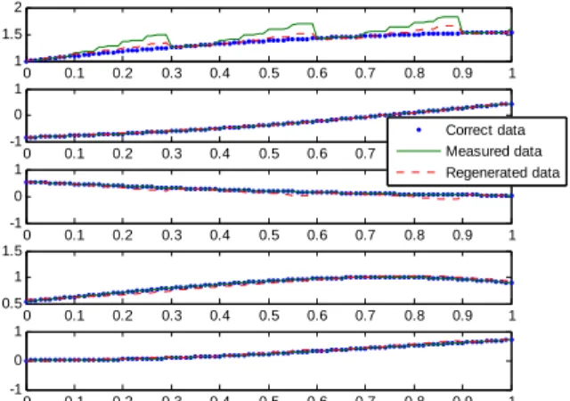
0 0.1 0.2 0.3 0.4 0.5 0.6 0.7 0.8 0.9 1 1 1.5 2 x1 0 0.1 0.2 0.3 0.4 0.5 0.6 0.7 0.8 0.9 1 -1 0 1 x2 0 0.1 0.2 0.3 0.4 0.5 0.6 0.7 0.8 0.9 1 -1 0 1 x3 0 0.1 0.2 0.3 0.4 0.5 0.6 0.7 0.8 0.9 1 0.5 1 1.5 x4 0 0.1 0.2 0.3 0.4 0.5 0.6 0.7 0.8 0.9 1 -1 0 1 x5 t Correct data Measured data Regenerated data
Figure 6 –Sensor value before and after the neural network in for a 5-7-2-7-5 network
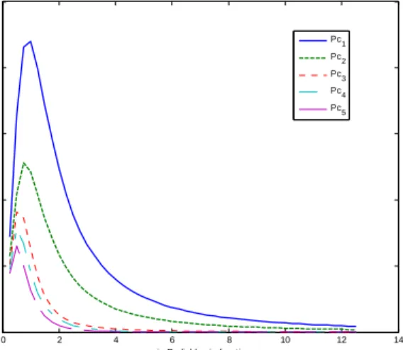
Since we have generated these data with a known function, we know that these data are originated from two independent sources but this is not the case for actual application of sensor fault diagno-sis. In these cases, Nonlinear PCA with KPCA algorithms can be used. In fact, the number of ma-jor principal components represents the number of independent variables. In order to show this fact in our sample data, the algorithm of KPCA is done with radial basis function as defined in Equation 12. The parameter of radial basis function,σ , is changed discretely from 1 to 12 and with each value the algorithm of KPCA is applied and the first 5 principal values are calculated. Figure 6
shows these values. It is obvious from this graph that the first two components have much more contribution to the variance of total data.
0 2 4 6 8 10 12 14 0 5 10 15 20 25
σ in Radial basis function
E igenv al ues of K ernel f unc ti on Pc1 Pc2 Pc3 Pc4 Pc5
Figure 6 –Nonlinear Principal values vs. σin radial
basis function 0 0.1 0.2 0.3 0.4 0.5 0.6 0.7 0.8 0.9 1 1 1.5 2 x1 0 0.1 0.2 0.3 0.4 0.5 0.6 0.7 0.8 0.9 1 -1 0 1 x2 0 0.1 0.2 0.3 0.4 0.5 0.6 0.7 0.8 0.9 1 0 0.5 1 x3 0 0.1 0.2 0.3 0.4 0.5 0.6 0.7 0.8 0.9 1 0.5 1 1.5 x4 0 0.1 0.2 0.3 0.4 0.5 0.6 0.7 0.8 0.9 1 -1 0 1 x5 t Correct data Measured data Regenerated data
Figure 7 –Sensor values before and after the fault diagnosis algorithm with KPCA
5.
Conclusion
In summary the problems of AANN as a method of Nonlinear PCA and as a technique for Sensor Fault Diagnosis are discussed and some useful strategies for finding the best architecture of AANN are suggested. Specially for the number of neurons in bottleneck layer which represents the number of independent imbedded variables we showed that if this number is more than the num-ber of independent variables the network does not work effectively for the purpose of sensor fault
diagnosis. Method of Kernel PCA is also dis-cussed and its pros and cons compared to AANN are studied. Since in the method of KPCA is a lazy algorithm and the reconstruction of the data form embedded variables needs very complicated com-putations and requires a nonlinear optimization, we suggested training of two neural network, for mapping and reconstructing respectively. Using these two networks in serial emulates an AANN and the numerical examples shows the better per-formance of this method.
References:
[1] Pearson K., On lines and planes of closest fit to systems of points in space Phil. Mag. 2, 1901 , 559–72
[2] Hotelling H., Analysis of a complex of statisti-cal variables into principal components J. Educ. Psychol., 1933, 24 417–41
[3] Bakshi B. R., Multiscale PCA with application to multivariate statistical process monitoring, AIChE J., Vo1 44, 1998, 1596-1610
[4]Gertler G. W., Li Y., Huang, and McAvoy T. Isolation enhanced principal component analy-sis. AIChE J., 1999, Vo1.45, 323-334
[5]Dunia R., Qin S. J., Subspace approach to multi- dimensional fault identification and re-construction. AIChE J., 1998, Vo1.44, 1813-1831
[6]Haiqing W., Zhihnan S., Ping L., Fault Detec-tion Behavior and Performance Analysis of PCA- based Process Monitoring Methods. Ind. Eng. Chem. Res., 2002, Vol. 41, 2455-2464 [7] Kramer M. A., Nonlinear Principal Component
Analysis using Autoassociative Neural Net-works. AIChE J., 1991, Vo1.37, 233-243 [8] Hines J. W., Wrest D.J. Uhrig R.E. Plant Wide
Sensor Calibration Monitoring. Proceedings of the 1996 IEEE International Symposium on Intelligent Control, Dearborn, MI September 15-18, 1996
[9] Mattern D.L., Jaw L.C., Guo T., Graham R. and McCoy W., Using Neural Networks for
Sensor Validation, 34th
IAA/ASME/SAE/ASEE Joint Propulsion Con-ference & Exhibit, July 13-15,1998 / Cleve-land, OH
[10]Antory D., Kruger U, Irwin G.W., McCul-lough G., Industrial process monitoring using nonlinear principal component models, Intelli-gent Systems, 2004. Proceedings. 2004 2nd International IEEE Conference, Volume 1, 22-24 June 2004 Page(s):293 - 298 Vol.1 [11] Mattern D.L., Jaw L.C., Ten H.G., Graham R.
and McCoy W., Simulation of an engine sen-sor validation scheme using an Autoassocia-tive Neural Network, AIAA/ASME/SAE/ASEE Joint Propulsion Conference and Exhibit, 33rd, Seattle, WA, July 6-9, 1997
[12]Huang J.; Shimizu H.; Shioya S. Data pre-processing and output evaluation of an Autoassociative neural network model for online fault detection in virginiamycin produc-tion Source:Journal of Bioscience and Bioen-gineering, Volume 94, Number 1, July 2002, pp. 70-77(8)
[13] Tan S., Mayrovouniotis M.L., Reducing data dimensionality through optimizing neural net-work inputs, AIChE Journal Volume 41, Is-sue 6, Date: June 1995, Pages: 1471-1480 [14]Scholkopf B. Smola A. Muller K.L.,
Nonlin-ear Component Analysis as Kernel Eigenvalue Problem. Neural Computation, Volume 10, Number 5, 1 July 1998, pp. 1299-1319(21) [15] Li W. Gong W., Liang Y. Chen W., Feature
Selection Based on KPCA, SVM and GSFS for Face Recognition Lecture Notes in Com-puter Science, 2005, no. 3687, pp. 344-350 [16] He Y. Zhao L. Zou C., Face Recognition
Based on PCA/KPCA Plus CCA, Lecture Notes in Computer Science, 2005, no. 3611, pp. 71-74
[17] Zhao, Q; Lu, H GA-Driven LDA in KPCA Space for Facial Expression Recognition Lec-ture Notes in Computer Science, 2005, no. 3611, pp. 28-36
[18]Lu B., Bi D., Tan J., A Method of Image De-noising Based KPCA, Infrared Technology, 2004, vol. 26, no. 6, pp. 58-61
[19] Kaieda K., Abe S., KPCA-based training of a kernel fuzzy classifier with ellipsoidal regions, International Journal of Approximate Reason-ing, 2004, vol. 37, no. 3, pp. 189-217
[20] Twining C.J., Taylor C.J., The use of Kernel Principal Component Analysis to model data
distributions. Pattern Recognition 36, 2003, 217-227
[21] Cho J., Lee J. Choi S. W., Lee D., Lee I.B., Sensor fault identification based on Kernel Principal Component Analysis., Proceedings of the 2004 IEEE International Conference on Control Applications, Volume 2 , 2-4 Sept., 2004,1223 - 1228 Vol.2
[22] Choi S. W., C. Lee and I.-B. Lee, “Fault de-tection and isolation of nonlinear processes based on kemel PCA”, Chemometrics and in-telligence Laboratory Systems
[23] Boser B. E., Guyon I. M., Vapnik V. N., A Training Algorithm for Optimal Margin Clas-sifiers., Proceeding of the 5th Annual ACM Workshop on Computational Learning The-ory., 1992, p144-152
[24] Vapnik V., Chervonenkis A., The Nature of Statistical Learning Theory., 1995, New York Springer-Verlag.