Wayne State University Theses
1-1-2016
Consensus Regularized Selection Based Prediction
Ping Wang
Wayne State University,
Follow this and additional works at:https://digitalcommons.wayne.edu/oa_theses
Part of theComputer Sciences Commons, and theStatistics and Probability Commons
This Open Access Thesis is brought to you for free and open access by DigitalCommons@WayneState. It has been accepted for inclusion in Wayne State University Theses by an authorized administrator of DigitalCommons@WayneState.
Recommended Citation
Wang, Ping, "Consensus Regularized Selection Based Prediction" (2016).Wayne State University Theses. 511.
by
PING WANG
THESIS
Submitted to the Graduate School
of Wayne State University,
Detroit, Michigan
in partial fulfillment of the requirements
for the degree of
MASTER OF SCIENCE
2016
MAJOR: COMPUTER SCIENCE
Approved By:
To my husband Tian and my parents.
First and foremost, I would like to thank my advisor Professor Chandan K. Reddy for all his guidance and assistant during my graduate studies, especially in this thesis. With his knowledge and experience, he provided me many valuable suggestions for this work. I also appreciate the collaborative environment he created in our research group to share the views and ideas, which are really helpful for me to learn more efficiently.
I am very fortunate to have Professor Zaki Malik and Professor Zichun Zhong as my com-mittee members. I appreciate them for taking their time to provide any valuable comments and evaluate this work.
I’ve been enjoying to work with the group members in the Data Mining and Knowledge Discovery (DMKD) Laboratory, which is a great group full of inspiring members. I would like to thank Yan Li for providing me many valuable suggestions. I would also like to thank Bhanukiran Vinzamuri and Karthik Padthe for sharing their ideas and knowledge with me and for their contribution in this work. I also appreciate my other lab mates for their patience and help.
Last but not the least, I would like to thank my husband Tian Shi for his love and un-derstanding. Many thanks are given to my parents for all their support and encouragement.
DEDICATION . . . ii
ACKNOWLEDGMENTS . . . iii
LIST OF TABLES . . . vi
LIST OF FIGURES . . . vii
CHAPTER 1 INTRODUCTION . . . 1
1.1 Motivation . . . 1
1.2 Related Literature . . . 3
1.2.1 Non-convex Regularized Linear Regression Models . . . 3
1.2.2 Additive Models . . . 4
1.2.3 Interactions based Models . . . 5
1.3 Contributions . . . 7
1.4 Thesis Organization . . . 8
CHAPTER 2 PROPOSED APPROACH . . . 9
2.1 Preliminaries . . . 9
2.2 Consensus Regularized Selection based Prediction Method . . . 12
2.3 Optimization . . . 16
2.4 Complexity Analysis . . . 20
CHAPTER 3 EXPERIMENTAL RESULTS . . . 21
3.1 Experimental Setup . . . 21
3.1.1 Electronic Health Records (EHRs) . . . 21
3.1.2 Synthetic Datasets . . . 23 3.2 Evaluation Metrics . . . 24 3.2.1 AUC . . . 24 3.2.2 MSE . . . 25 3.2.3 R2 . . . . 26 3.3 Implementation Details . . . 26 iv
3.5 Scalability Experiments . . . 30
3.6 Comparison with Clinical Models on EHRs . . . 32
3.6.1 Clinical Relevance . . . 32
3.6.2 Risk Calibration Plots . . . 33
CHAPTER 4 CONCLUSION AND FUTURE WORK . . . 36
REFERENCES . . . 37
ABSTRACT . . . 42
AUTOBIOGRAPHICAL STATEMENT . . . 44
Table 1.1 Commonly used Non-Convex penalties. . . 3 Table 2.1 Notations used in this thesis. . . 9 Table 3.1 Description of the EHRs and synthetic datasets used in our experiments. 21 Table 3.2 Confusion matrix for a binary-class problem. . . 24 Table 3.3 Performance comparison of CRISP with different models using AUC ±
std for 30-day readmission problems on longitudinal EHRs. . . 28 Table 3.4 Performance comparison of CRISP with machine learning models using
MSE± std for the 30-day readmission problem on longitudinal EHRs. . 28 Table 3.5 Performance comparison of CRISP with machine learning models using
MSE± std on synthetic datasets. . . 29 Table 3.6 Performance comparison of CRISP with machine learning models using
R2 on synthetic datasets. . . 29 Table 3.7 AUC comparison of our approach with clinical models for 30-day and
365-day readmission problems on HF-cohort data. . . 34
Figure 1.1 Plots of commonly used Non-Convex penalties when λ= 1 and γ = 3. . 4 Figure 2.1 Illustration of CRISP Algorithm applied on EHRs. . . 20 Figure 3.1 Class distribution in EHR datasets. . . 22 Figure 3.2 Performance comparison of CRISP with various state-of-the-art methods
for the 365-day readmission problem on longitudinal EHR datasets. . . 30 Figure 3.3 Comparison of time taken in seconds for three different non-convex
reg-ularizers compared to MC+ with increasing dimensionality of the features. 31 Figure 3.4 Calibration plots for CRISP on HF-cohort data for (a) 30-day, (b)
365-day readmission problems. . . 34
CHAPTER 1
INTRODUCTION
1.1
Motivation
Consensus modeling is an important topic which deals with assembling a committee of experts for a given problem and then obtaining a consensus among their votes to arrive at the final prediction. This has been applied to predictive analytics problems such as classi-fication, ensemble modeling and active learning where a committee of models are created to cast their individual votes on a test case. Multiple Classifier Fusion is an application of consensus modeling where multiple classifiers are integrated within a single framework [1]. The effectiveness of consensus modeling in such scenarios like classification and active learn-ing relies on the mechanism used to build the committee of models. Query by Committee is also a well studied topic in the context of active learning, where consensus modeling is used to determine the instance whose label must be queried [2, 3]. Consensus modeling can be extended to the field of regularization in the context of regression which is described to be the consensus regularization problem in this thesis.
Consensus regularization is the problem of identifying an optimal regularizer for a given regression problem among a set of regularized models by obtaining a consensus among all these models. The consensus among all the models is obtained using a pre-defined criterion, which assesses each of the candidate regularizers separately and decides the best candidate regularizer for prediction. Solving such a problem is non-trivial, as it is not easy to integrate multiple regularizers within a single framework. This is because the regularizers differ in their degree of complexity and how they interpret the inherent data structure which makes this problem of integration highly cumbersome. Optimization methods such as proximal algorithms [4] also cannot be universally applied to solve multiple regularization problems, as the cost of obtaining the proximal operator associated with each regularizer may significantly differ [5]. Finally, ensuring diversity of regularizers within a multiple regularizer framework is not always guaranteed. This is the reason why the problem of unifying multiple regularizers has not received much attention in the data mining community.
To efficiently solve this problem, in this thesis, we propose a two-step algorithm. The first step generates a committee of regularization models. Each model in this committee differs from the others, but the solution for each one of them can be expressed using a unique generalized thresholding operator [6–8]. The advantage of our approach is that this generalized thresholding operator can be computed efficiently for each individual model. In addition, to promote robustness in the model to capture sparsity more efficiently, we use non-convex regularizers within our approach. Non-convex regularizers have certain unique advantages of unbiased feature selection and consistent results which make them a better choice compared to the prominent sparsity promoting convex regularizers such as the Lasso. We choose a non-convex regularizer called the minimax concave plus (MC+) penalty for the model proposed in this thesis which is explained in Chapter 2.
The second stage of our approach involves using a consensus criterion among all these candidate regularizers to obtain the final model for prediction. A major advantage of our approach is that an expert can design an arbitrary consensus criterion and integrate it with this approach to obtain an optimal model for prediction. This is particularly important while building prediction models on real-world data where an expert aims at optimizing the model performance for domain-specific metrics.
We conduct exhaustive empirical evaluation of this Consensus RegularIzed Selection based Prediction framework (CRISP) algorithm on electronic health records (EHRs) col-lected from a large hospital consisting of 8,000 patient records and various synthetic datasets. Our extensive set of experiments indicate that CRISP outperforms several state-of-the-art methods such as additive models and other competing non-convex regularized linear regres-sion methods. In addition, we establish the clinical relevance of CRISP on EHR datasets by comparing it with four widely used clinical models which affirms the importance of this approach.
1.2
Related Literature
In this section, we review the existing works related to the topics of non-convex regularized linear regression, additive and interactions based methods. We briefly mention how the contributions in this thesis are distinctly different from these algorithms that are available in the literature.
1.2.1
Non-convex Regularized Linear Regression Models
Usually, the problem of recovering a sparse signal representation according to a signal dictionary can be formalized as a penalized least-squares problem in which sparsity is usually induced by a convex penalty on the coefficients, including the`1norm,`2norm and the elastic net penalty functions. Based on some empirical studies, these approaches perform well in most scenarios, however, it has also been observed that they are not perfect in capturing sparsity. In contrast, methods with non-convex penalties can recover sparsity more efficiently and are being actively pursued by researchers recently [9–11]. Table 1.1 and Figure 1.1 give an overview of some well known non-convex penalties commonly used in the literature. MC+ penalty is the non-convex penalty used in our work and will be discussed in detail in Chapter 3.
Table 1.1: Commonly used Non-Convex penalties.
Name P(βi) SCAD λR|βi| 0 min(1, [γλ−x]+ (γ−1)λ )dx (γ >2) LSP λlog(1 +|βi|/γ) (γ >0) Capped-`1 λmin(|βi|, γ) (γ >0)
Smoothly Clipped Absolute Deviation (SCAD), proposed by Fan and Li [12], corresponds to a quadratic spline function with knots at λ and γλ. This penalty function leaves large values ofβi not excessively penalized and makes the solution continuous. Log-Sum Penalty (LSP) has slope at the origin that grows roughly as 1/γwhenγ →0, which allows a relatively large penalty to be placed on small nonzero coefficients and more strongly encourages them to be set to zero [13]. In other words, LSP has the potential to guarantee more sparsity
than the `1 norm. Capped-`1 penalty, which is a simpler but less smooth version of the SCAD regularization, is a good approximation to `0 as γ → 0 [14]. This means that its regularization condition is equivalent to `0 regularization up to a rescaling of λ. Capped-`1 penalty treatsβi equally, if|βi|is bigger thanγ, which makes it more robust to outliers than the `1 norm.
Figure 1.1: Plots of commonly used Non-Convex penalties when λ= 1 and γ = 3.
In order to efficiently solve methods with these non-convex penalties efficiently, optimiza-tion methods such as Difference of Convex Funcoptimiza-tions (DC) [15] programming, Alternating Direction Method of Multipliers (ADMM) [16] and proximal algorithms [4] are popular choices.
1.2.2
Additive Models
Generalized Additive Models (GAM), which usually model the dependent variable y as a sum of univariate models of each feature xi, have the form of
g(E[y]) =Xfi(xi) =F(x) (1.1)
where g(·) is the link function. Individual terms in GAM can be represented by a variety of functions, including splines, regression trees, or tree ensembles [17]. We want to find the
best model F(x) that minimizes the following objective function:
minFE[L(y, F(x))] (1.2)
whereL(·,·) is a non-negative convex loss function. There are two popular methods of fitting GAM: Backfitting and gradient boosting [17]. GAM have the ability to capture non-linear relationship between individual features and the response, however, it does not perform as well as the full complexity models since it does not model any interactions between features. To overcome the disadvantage of GAM, generalized additive models plus interactions (GA2M), adding selected terms of interacting pairs of features to GAM, is proposed as follows:
g(E[y]) =Xfi(xi) +
X
fij(xi, xj) (1.3) In other words, GA2M consist of both univariate terms and a small number of pairwise interaction terms. The interaction terms set can be determined by a greedy forward selection strategy [18] for low-dimensional data and FAST interaction detection can be used for large high-dimensional data [17, 19, 20].
1.2.3
Interactions based Models
Additive models which only consider the main effects of the features are ineffective in many situations when predicting an outcome of interest [21]. Considering the application in medical diagnosis, the co-occurrence of two symptoms may be more helpful for when two symptoms are considered together, it will be highly predictive of the disease than the situation in which only one symptom presents. In this case, the interaction between these two symptom variables are positive. On the other hand, if both of the variables provide redundant information about the disease to the doctor, there will be a negative interaction between them. In this situation, knowing both symptoms does not provide more information about the status of the disease than knowing only one of them. In such application, it is desirable to identify the main factors which lead to the disease.
response variable except for the main effects, are more effective than the additive models. It should be noted that interactions between two variables are different from the correlation between them. Correlation [22] between two variables means that the values of one variable is related in some way to the values of the other. It indicates that the values of one variable will generally co-occur with some certain values of the other. While interaction [23] between two variables means that the effect of one variable on the response variable differs at different values of the other. Whether two variables interact on the response variable says nothing about whether they are correlated, and vice versa. However, it is challenging to fit regression models with interactions when one has even a moderate number, m, of measured features, since there are mk interactions of order k. Hiernet method considers the pairwise (k = 2) intersection in the model.
The regression model in hiernet method [21], with pairwise interactions between features, has the form of
Y =β0+ X j βjXj + 1 2 X j6=k ΘjkXjXk+ (1.4) where∼N(0, σ2),β ∈
Rm, and Θ = [Θjk]∈Rm×m is the interaction coefficients matrix. In
these models, the linear component represents the main effect terms and the quadratic part corresponds to the interaction terms. In general, not all of the main effects and interactions are of interest, thus it is critical to select the variables of high significance. In statistics, a hierarchical structure between the main effects and interaction effects has been shown to be very effective in constraining the search space and identifying important individual features and interactions. Specifically, the hierarchical constraint requires that an interaction term is selected in the model only if the main effects are included.
The goal of hiernet method is to estimate β and Θ, which satisfies Θ = ΘT and Θ jj = 0. The factor of one half in front of the interaction part is to deal with the symmetric matrix Θ of interactions. Strong theoretical properties have been established for such hierarchical models [21]. In Statistics, there are two types of restrictions on the interaction terms: strong hierarchy ( ˆΘjk 6= 0⇒βˆj 6= 0 and ˆβk = 0) and weak hierarchy ( ˆ6 Θjk 6= 0 ⇒βˆj 6= 0 or ˆβk 6= 0).
We refer to these algorithms which model strong and weak interactions, in this thesis, as hiernet-strong and hiernet-weak, respectively.
In the hiernet model, the number of main effect are m and the number of interaction variables arem(m−1)/2. The goal is to select a subset, which is predictive of the outcome, from the main effect and interaction terms and to estimate the values for the nonzero param-eters of the model. The convex optimization problem using lasso to estimate the paramparam-eters will be as follows.
minβ,φ1
2 ky−β01−Xφe k 2
+λkφ k1 (1.5) where 1 ∈ Rn is the vector of ones, φT = [βT, vec(Θ)T]. Hiernet method uses a lasso-like procedure which adds a set of convex constraints to the lasso and produces sparse estimates of β and Θ while satisfying the strong and weak hierarchy constraints [21].
In contrast to these methods, our CRISP approach uses a non-convex penalty generating multiple candidate models in the process, and selects an optimal model using a consensus criterion among these candidate models for the final prediction.
1.3
Contributions
In order to build predictive models with lower variance and better generalization, we build a committee of regularized linear regression models by considering a non-convex regulerizer in the model and integrates them with a consensus criterion to select the best model for final prediction. Thus the main contributions of this thesis can be summarized as follows.
• Propose a Consensus RegularIzed Selection based Prediction framework (CRISP) which builds a committee of non-convex regularized linear regression candidate models and integrates them with a consensus criterion to obtain the optimal model for prediction.
• Develop an efficient cyclic coordinate descent based solution for the optimization prob-lem being solved while learning each candidate model in CRISP. We also provide the proof of convergence.
regu-larized linear regression models using metrics such as AUC, MSE and R2. We also conduct experiments to assess the performance of CRISP on high-dimensional syn-thetic datasets. In addition, we evaluate the performance of the CRISP algorithm on Electronic Health Records (EHR) datasets with respect to four widely used clinical models to establish its clinical relevance.
1.4
Thesis Organization
The thesis is organized as follows. Chapter 1 introduces the motivation of the thesis and provides a brief review of the related work on additive, hierarchical and non-convex regularized regression models. In Chapter 2, first we provide the notations that are necessary for understanding the proposed CRISP model along with a brief overview of regularization theory. In addition, we present the details of the CRISP model including the minimax concave plus (MC+) penalty, the generalized thresholding operator and the corresponding cyclic coordinate descent algorithm employed to optimize the CRISP method. In Chapter 3, we evaluate the performance of CRISP using various additive, interactions and non-convex regularized linear regression methods on both EHR dataset and synthetic datasets. Finally, we conclude our discussion and provide directions for future work in Chapter 4.
CHAPTER 2
PROPOSED APPROACH
In this chapter we introduce our proposed consensus regularized selection based prediction method. As discussed in previous chapter, the problem of obtaining a consensus among such diverse regularizers is extremely important in order to determine the optimal regularizer for the model. Therefore, the main objective of this chapter is to build a committee of regularized linear regression models by considering a non-convex regulerizer in the model and integrates them with a consensus criterion to select the best model for final prediction. Before we discuss the algorithm in detail, the preliminaries of the proposed method will be briefly presented.
2.1
Preliminaries
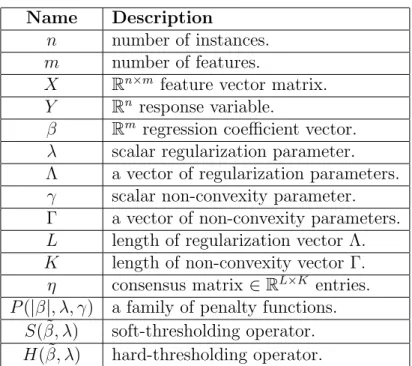
This section introduces the preliminaries required to comprehend the proposed approach. First, the notations used in our work are presented in Table 2.1. We then review the concepts associated with regularized linear regression models followed by introducing the thresholding operators used in our CRISP algorithm.
We now consider the basic linear regression model
Table 2.1: Notations used in this thesis.
Name Description
n number of instances. m number of features.
X Rn×m feature vector matrix. Y Rn response variable.
β Rm regression coefficient vector. λ scalar regularization parameter. Λ a vector of regularization parameters. γ scalar non-convexity parameter. Γ a vector of non-convexity parameters. L length of regularization vector Λ. K length of non-convexity vector Γ. η consensus matrix ∈RL×K entries. P(|β|, λ, γ) a family of penalty functions.
S( ˜β, λ) soft-thresholding operator. H( ˜β, λ) hard-thresholding operator.
Y =f(X) = Xβ+. (2.1)
which aims at estimating the relationship between the features X = (x1, x2, ..., xn)T and the corresponding response variable Y = (y1, y2, ..., yn)T, where xi ∈ Rm and yi ∈ R for i= 1, . . . , n. In high-dimensional data, m is much greater thann. This motivates the use of a relatively small number of predictors to accurately predict the outcome. Fitting regression models for all subsets of predictors and then selecting the best one is challenging when there are even a moderate number of predictors, since the total number of all the possible subsets isPm
k=1 m
k
. Most of the existing methods aim at learning the parameters of the model and selecting the variables simultaneously by solving the following minimization problem.
ˆ β = arg min β∈Rm 1 2 n X i=1 (yi−f(xi))2+λP(β) (2.2)
where λ is the penalty coefficient which controls the degree of regularization and P(β) is a penalty function.
A number of variable selection methods with convex penalty functions and the corre-sponding optimization methods have been proposed in the literature [24–26]. A popular choice is to use the family of `p-norm penalty functions. Generally, if we use the`p penalty with p > 1, the solution is not sparse. When p < 1 the solution is sparse, but the cor-responding problem is non-convex. Lasso [26, 27] with the `1 penalty function is convex and non-smooth which produces models with good prediction accuracy when the underlying model is reasonably sparse. The lasso penalty is often considered as the convex surrogate for the best-subset selection with the `0 penalty, k β k0= Pmi=1I(|βi|>0), which penalizes the number of non-zero coefficients in the model, where Irepresents the indicator function. However, there are two disadvantages for the lasso model. One is that some experimen-tal results show that the `1 penalty tends to generate biased estimates for large coefficients, which may prevent its consistent variable selection. In addition, lasso is effective at giving sparse solutions but when variables are correlated, it excludes many correlated variables once a strong variable is included and fully fitted in the model. Also, when the regularity
conditions are violated, the lasso can be sub-optimal in variable selection, which means it can fail as a variable selector. In order to include the full effect of a variable in the model, we have to relax the penalty to allow the other redundant but possibly correlated features. Fan and Li [12] suggested some desirable properties of the penalization function, such as sparsity, continuity and unbiasedness of the estimated parameters. In order to satisfy all the good properties of the penalty function, some non-convex penalty functions, which bridge the gap between `1 and `0 penalty, have been considered.
ˆ β = arg min β∈Rm 1 2 n X i=1 (yi−f(xi))2+λP(β;γ) (2.3)
where P(β;γ) defines a family of penalty functions concave in |β|, where |β| represents a vector consisting of the absolute values of the regression coefficient vector β and γ is a scalar user given non-convexity parameter. In the optimization problem shown in Eq. (2.3), both λ and γ are user parameters and they control the degree of the regularization and non-convexity, respectively. In other words, for a fixed λ, there will be a family of penalty functions, each of which corresponds to an optimization problem. This means that the penalty functionP(β;γ) can be updated to beP(β;λ, γ) if we also considerλas a parameter of the model. In addition, due to the fact that the penalty function is separable for the parameters β = (β1, ..., βm)T, the optimization problem in Eq. (2.3) can be updated as follows after adding λ in the penalty function.
ˆ β = arg min β∈Rm 1 2 n X i=1 (yi−f(xi))2+ m X i=1 P(|βi|;λ;γ) (2.4)
In this optimization problem described in Eq. (2.4), for a fixed λ, the value of the pa-rameter γ varies in the range of [1+,∞] where 1+ represents values greater than 1. Each variation of γ corresponds to a separate problem. A family of threshold operators called the generalized thresholding operator [6–8], with soft-thresholding (ST) and hard-thresholding (HT) as its two extremes, will be obtained by solving all the optimization problems using the cyclic-coordinate descent method [28].
Also, the regularization parameterλcan vary, which generates different families of thresh-old operators. Each threshthresh-old operator corresponds to a solution of an optimization model with a specific λ and γ values. This means a consensus matrix η will be obtained based on the family of threshold operators obtained by varying λ and γ. This matrix captures the information across all the different regularization models in the committee. Subsequently, we use a consensus criterion to select the best set of model parameters from this matrix. We now present the optimization involved in the CRISP algorithm along with its proof of convergence and a discussion of the algorithm complexity in the next section.
2.2
Consensus Regularized Selection based Prediction Method
In this section, we introduce the properties of the minimax concave plus (MC+) penalty function used in CRISP first. We then propose a consensus regularized selection based pre-diction method which generates a committee of regularized models and among them selects the best model. The selection among these different models is done using a decision rule which is different from the standard majority voting based methods employed in the classifi-cation literature. Majority voting is a binary decision rule and it selects the candidate which obtains the highest number of votes. In other words, majority voting takes all the different choices into consideration by counting the occurrence when making decisions. However, in our method, we conduct an explicit search for the optimal model parameters (λ∗, γ∗) among all the entries in the consensus matrixηwhich effectively captures the information across all the different models.
The non-convex penalty used in our work is the minimax concave plus (MC+) penalty which is a fast, continuous, nearly unbiased and accurate method for penalized variable selection in linear regression [10]. The minimax concave plus (MC+) penalty is defined by
P(β;λ;γ) = λ Z |β| 0 (1− x γλ)+dx (2.5) =λ(|β| − β 2 2λγ)I(|β|< λγ) + λ2γ 2 I(|β| ≥λγ)
γ varies from ∞ to 1. (·)+ represents the positive component. The threshold operators for the MC+ penalty will form a continuum between the soft- and hard-thresholding functions, which generates a natural and smooth transition across the set of solutions. In addition, we can also vary the value of λ, which will determine a specific model along with the non-convexity parameter γ. Thus, using the MC+ penalty we will develop a committee of prediction models to be used in our CRISP model.
By using the MC+ penalty, we can consider different combinations of the regularization parameter (λ) and the non-convexity parameter (γ), which will be helpful to avoid obtaining sub-optimal solutions. In other words, the MC+ penalty ensures a family of models for a fixedλby interpolating between the`0norm and`1norm, which provides more candidates for approximation of the`0 norm. In addition, it also generates a series of thresholding operators with soft-thresholding operator and hard-thresholding operator as its two extremes. Thus, we can conclude that the MC+ penalty has the necessary and meaningful properties for capturing sparsity more efficiently.
Non-convex penalties such as the MC+ penalty perform better feature selection. When we use the MC+ penalty in the objective function in Eq. (2.6), the univariate penalized least squares objective function will be strictly convex, which ensures the descent property with coordinate descent method and the solution converges to a stationary point [10, 29]. We will now discuss our CRISP algorithm and provide the proof of convergence as well.
The objective function in Eq. (2.4) with the MC+ penalty is separable, which enables us to optimize the univariate case which is one-dimensional with the form
Q(1)(β) = 1 2(β− ˜ β)2+λ Z |β| 0 (1− x γλ)+dx (2.6)
using the standard coordinate-decent approach. If β > 0, the derivative of Q(1)(β) with respect to the β can be calculated as
dQ(1)(β)
dβ =β−
˜
β+λ(1− β
A similar expression can be calculated for the case β <0. Thus, the threshold operator for the MC+ penalty will be given by
Sγ( ˜β, λ) = arg min β Q (1)(β) (2.8) = 0 |β˜| ≤λ sgn( ˜β)(|1β˜−|−1λ γ ) λ <|β˜| ≤λγ ˜ β |β˜|> λγ
For a fixedλ, asγ varies, this generates a family of threshold operatorsSγ(·, λ) :R→R, with the soft and hard threshold operators as its two extremes. The soft-thresholding operator when γ → ∞ is given by Sγ( ˜β, λ)→S( ˜β, λ) (2.9) = arg min β { 1 2(β− ˜ β)2 +λ|β|} =sgn( ˜β)(|β˜| −λ)+
and the hard-thresholding operator when γ → 1+ for the one-dimensional optimization problem is in the form of
Sγ( ˜β, λ)→H( ˜β, λ) (2.10) = arg min β { 1 2(β− ˜ β)2+λI(|β|>0)} = ˜βI(|β˜|> λ)
Eq. (2.10) indicates that the hard-thresholding operator, which is conventionally used for the non-convex `0 penalty problem, can also be obtained as the limit of a sequence of Sγ( ˜β, λ) as γ → 1+. Since soft and hard thresholding functions are often used in the optimization problems with `1 and `0 penalty, we assume γ`1 = ∞ and γ`0 = 1+ for `1 and `0 norms,
respectively.
Eq. (2.8) for the univariate problem. In each iteration, all of themcoefficients are repeatedly updated until convergence. In this case, all the solutions when varying λ and γ will form a two-dimensional solution surface whose coordinates can be represented as the matrixη. The goal of our work is to find optimal parameters (λ∗, γ∗) corresponding to the best solution. In order to find the best solution, our method will evaluate each solution. We now present the consensus criterion used in our CRISP algorithm.
Consensus criterion: Squared error (se) of an estimator measures the square of the errors or deviations and assesses the quality of an estimator. It is used for assessing the performance of an estimator or a predictor. Generally, for the ith training instance (x
i, yi) and a linear fit ˆfλ`,γk(xi) =xiβˆλ`,γk, when the values ofλ` andγk are fixed, the squared error
of the predictor will be given below.
ηλ`,γk =se( ˆfλ`,γk) = n X i=1 ( ˆfλ`,γk(xi)−yi) 2 (2.11)
Using this formulation of the consensus criterion, we can evaluate the performance of each model for different pairs of (λ`, γk). We now present the CRISP algorithm which generates a family of solutions ˆβλl,γk to Eq. (2.4) and selects the best one using this criterion based
on the squared error of deviances. We assume that the matrix X is standardized with each column with zero mean and unit `2 norm. When γ =∞, the exact solution path for Q(β) using coordinate-descent method will be used as a warm start for the minimization of Q(β) with a non-convex penalty function.
The value of γ is decreasing until we have the solution path across a grid of values for γ [29]. The details of our approach are given in Algorithm 1. The univariate sub-problem in Eq. (2.6) will be optimized using coordinate descent method [28], which is a widely used non-derivative optimization algorithm. In each iteration of the coordinate descent method for the objective function, arg minβQ(β1, β2, . . . , βm), it performs search along one coordinate direction at the current point and cyclically iterates through the other directions. In other words, in each iteration, the algorithm solves the optimization problem as shown in Eq.(2.12)
for each variable βi(i= 1,2, ..., m) of the problem.
βik+1 = arg min u∈R
Q(β1k+1, ..., βik−+11, u, βik+1, ..., βmk) (2.12)
That is, in each iteration of the optimization problem, each variableβi(i= 1,2, ..., m) will be updated until convergence. Coordinate descent method minimizes a multivariable objective function by solving a series of univariate optimization problems in a loop.
2.3
Optimization
In this section, we discuss the optimization involved in the CRISP algorithm and also provide a detailed algorithmic description. We begin by providing the proof of convergence. The convergence of CRISP algorithm cannot directly follow the convergence property of coordinate-descent for functions with the form of the sum of a smooth loss function and a separable non-smooth convex penalty function due to its non-convex formulation. The coor-dinate decent method updates the variables using Eq. (2.12) until convergence is observed. CRISP algorithm always converges to a minimum of the objective function under certain conditions which will be discussed below.
Consider the criterion in Eq. (2.4), where the data (X, Y) lies on a compact set and no column of the features in X is a multiple of the unit vector. Also, suppose that the penalty functionP(β;λ;γ) is symmetric around 0, which means that it satisfiesP(β;λ;γ) = P(−β;λ;γ); the first derivative ofP(β) with respect toβ,P0(|β|), is non-negative, uniformly bounded and the second derivative P00(|β|) satisfies infβP
00
(|β|)>−1; the sequence gener-ated {βk}
k is bounded; for all the subsequences {βnk}k of {βk}k, the successive differences, i.e. (βnk−βnk−1) converges to 0.
Theorem 1 The univariate problem in Eq. (2.6) is strictly convex and the sequence of coordinate-updates {βk}k converge to a minimum solution of Eq. (2.4).
Proof. It should be noted that the MC+ penalty used in our work can meet all the required properties mentioned above. In addition, the assumption on data (X, Y) is used to ensure that the variables can be standardized and the non-degeneracy assumption onX means that
all the columns are identically non-zero.
For a fixed i and (β1,· · ·, βi−1, u, βi+1,· · · , βm), we denote Q(u) as
Q(u) = Qi(β1,···,β
i−1,u,βi+1,···,βm)
=l(β1,· · · , βi−1, u, βi+1,· · · , βm) +P(|u|)
(2.13)
where l(·) is the loss function. Then, based on the Taylor’s series expansions on f and penalty function P(|u|), the sub-gradient at uwill be
∂Q(u) =Q(u+δ)−Q(u) (2.14) =Oil(β1,· · · , βi−1, u, βi+1,· · ·, βm) +P 0 (|u|)sgn(u) =l(β1,· · · , βi−1, u+δ, βi+1,· · · , βm) −l(β1,· · · , βi−1, u, βi+1,· · · , βm) +P(|u+δ|)−P(|u|) =Oil(β1,· · · , βi−1, u, βi+1,· · ·, βm)δ+ 1 2δ 2 O2il +P0(|u|)(|u+δ| −(|u|)) + 1 2P 00 (|u∗|)(|u+δ| − |u|)2 where δ ∈ R and O2
il = 1 since it is the second derivative of the function f with respect to the ith coordinate. |u∗| is some number between |u+δ| and |u|. Assume that u0 is the optimal value for F(u), based on Eq. (2.14), we can have
Q(u0+δ)−Q(u0) (2.15) ≥ 1 2δ 2 O2il+ 1 2P 00 (|u∗|)(|u0+δ| − |u0|)2 ≥ 1 2δ 2O2 il+ 12P 00 (|u∗|)δ2 if P00(|u∗|)≤0 1 2δ 2O2 il+ 0 if P 00 (|u∗|)≥0 ≥ 1 2δ 2( O2il+min{P 00 (|u∗|),0})
Since for the MC+ penalty, infβP 00 (|β|) = −1 γ with γ > 1, O 2 il +infxP 00 (|x|) > 0. Then there exists a positive value θ = 12δ2(O2
il+min{infxP
00
(|x|),0}) such that
Q(u0+δ)−Q(u0)≥θδ2 (2.16)
Based on the analysis above, the boundedness of the sequence βt for t >1 will be
Q(βit−1)−Q(βit+1−1)≥θ(βit+1−1−βit+1)2 (2.17) =θ kβit−1−βit+1−1 k2
2
where βit−1 = (β1t,· · · , βit, βit+1−1,· · · , βmt−1). Using this boundedness for each coordinate, for every t, we will have
Q(βt+1)−Q(βt)≥θ k(βt+1−βt)k22 (2.18) From Eq. (2.18), we can see that the decreasing sequence Q(βt) converges. The sequence βk cannot cycle without convergence and it must have a unique limit point. This completes the proof of convergence for βk.
We now provide a stepwise description of the CRISP algorithm. Algorithm 1 outlines the CRISP algorithm for selecting the best estimates among a family of solutions ˆβλ`,γk to
Eq. (2.4). A grid of increasing Λ = {λ1, λ2,· · · , λL, λL+1} and Γ = {γ1, γ2,· · · , γK} values are used for traversing different combinations of λ and γ and generating different candidate models in the ensemble. Here, the additionalλL+1values is used for the warm start of CRISP algorithm by Lasso.
In lines 2-3, we initialize the estimator using the solution from Lasso for the minimization of Q(β) at a smaller value of γ corresponding to a more non-convex penalty. In lines 4-8, each element of the coefficient vector is updated using the coordinate-wise update as shown in Eq. (2.8) until the solutions converge to the solution for Eq. (2.4) when λ = λ` and γ = γk. In line 10, we evaluate each model by obtaining the value of the squared error se
and populate aL×K consensus matrixη, in whichηλ`,γk =se( ˆfλ`,γk) for`= 1,2,· · · , Land
k = 1,2,· · · , K. Here L and K represent the number of elements in Λ and Γ, respectively. In Line 13, according to the value of the se, the best model parameters which has the minimumsevalue among theLK entries in ηwill be selected as the final model parameters. Subsequently, the model β∗ corresponding to these paramaters (λ∗, γ∗) will be used for prediction. It should be noted that the model selection in CRISP algorithm is done based on the training data.
Algorithm 1: CRISP Algorithm
Input: Predictor matrix (X); response variable (Y); regularization parameter vector (Λ); non-convexity parameter vector (Γ), length of Λ(L), length of Γ(K).
Output: Optimal model parameters (λ∗, γ∗) and regression coefficient vector (β∗). 1 for ` =L,· · · ,2,1do
2 Use Lasso solution ˆβλ`+1,γK as warm start; 3 Initialize ˜β ←βˆλ`+1,γK; 4 for k =K,· · · ,2,1 do 5 repeat 6 for i= 1,2,· · · , m do 7 β˜i ←Sγk( ˜β, λ`) using Eq. (2.12); 8 end 9 until β˜ converges to βˆλ`,γk;
10 Estimateηλ`,γk using Eq. (2.11) for ˆβλ`,γk ;
11 end
12 end
13 (λ∗, γ∗)←arg minλ`,γk∈Rη ;
14 Select final model β∗ corresponding to (λ∗, γ∗) ;
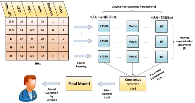
In Figure 2.1, we provide an illustration of our CRISP algorithm applied on Electronic Health Records (EHRs) to predict the readmission risk of patients [30, 31]. The algorithm initially learns a soft-thresholding based solution (Lasso) to begin the process of creating an ensemble of non-convex models by varying the non-convexity parameter γ and the reg-ularization parameter λ to generate a two-dimensional surface of solutions. As γ is varied, we obtain a unique non-convex model. These models are then integrated using a consensus criterion which determines the best pair of regularization (λ) and non-convexity (γ)
param-Model Evaluation by Clinician H( ,λ) = ɪ(| | λ) Select Optimal (ɣ,λ) 12.5 10 8 24 1 0 14.5 14 6.2 26 0 1 17 17 9 29 1 0 19 18 8.3 28 1 1 11 14 4.1 32 1 0 Consensus criterion (se) S( ,λ) = sgn( )(| |-λ)+ Final Model Sparse Learning EHRs
Varying Non-convexity Parameter(ɣ)
LASSO . . . Modeli . . . HT LASSO . . . Modeli . . . HT LASSO . . . Modeli . . . HT Varying regularization parameter (λ) . . . . . .
Figure 2.1: Illustration of CRISP Algorithm applied on EHRs.
eters. The consensus criterion is a user-defined criterion and it helps to optimize the search space among different models to choose the best model for prediction. Once the final set of parameters are obtained the corresponding model is chosen as the final model for prediction.
2.4
Complexity Analysis
CRISP uses a cyclic coordinate descent based method to generate a committee of regu-larized models. The selection procedure using the squared error criterion for different (λ`, γk) values takes linear time in general, as we have to find the minimum entry among a set ofLK entries in the consensus matrix η. Filling up each entry of the matrix η constitutes O(m) time. When (λ∗, γ∗) are selected, these model parameters are used for the final prediction. Hence, the overall time complexity of the CRISP algorithm is O(nm).
CHAPTER 3
EXPERIMENTAL RESULTS
In this chapter, we conduct different experiments to evaluate the performance of the CRISP algorithm. We evaluate the goodness of prediction, parameter sensitivity and scal-ability of CRISP by comparing it with various state-of-the-art algorithms. In addition, the CRISP algorithm is also compared with the clinical models in practice on Electronic Health Records (EHRs) datasets to assess its clinical relevance, and our results demonstrate the superior performance of the CRISP algorithm. Finally, we show the risk calibration plots which illustrate the agreement between predicted and observed risks on EHR datasets.
3.1
Experimental Setup
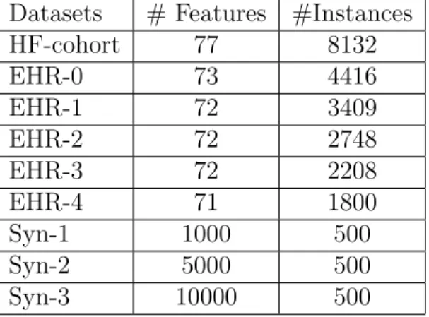
We evaluate the performance of our CRISP algorithm using real-world EHRs and syn-thetic datasets which are summarized in Table 3.1.
Table 3.1: Description of the EHRs and synthetic datasets used in our experiments. Datasets # Features #Instances
HF-cohort 77 8132 EHR-0 73 4416 EHR-1 72 3409 EHR-2 72 2748 EHR-3 72 2208 EHR-4 71 1800 Syn-1 1000 500 Syn-2 5000 500 Syn-3 10000 500
3.1.1
Electronic Health Records (EHRs)
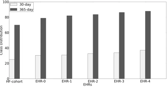
The EHRs used in this thesis were obtained from Henry Ford Health System in Detroit, Michigan in United States for patients admitted with chronic heart failure (CHF) condition over a period of 10 years. In Figure 3.1, we depict the class distribution for these EHRs. The y-axis represents the % of readmissions (positive class) for 30-day and 365-day readmission. The x-axis represents the indices of the EHRs. These EHRs were procured over successive readmissions of patients. The suffix next to EHR represents the index of readmission, for example EHR-irepresents all sets of patients readmitted for theith time. It can be observed
that the number of patients in each of the longitudinal EHRs decreases with successive readmissions. In addition to the readmission datasets, we also use a basic cohort dataset (HF-cohort) which represents an aggregated dataset summarizing the readmission information for all individuals over 10 years.
Figure 3.1: Class distribution in EHR datasets.
The feature groups that were included for our evaluation include medications, procedures, labs, demographics and comorbidities [32]. Here, we summarize the main data pre-processing methods[33, 34] used when generating the EHR dataset. We create binary variables from the procedures and medications list which indicate the presence or absence of that particular procedure or medication for the patient. For the labs, we apply the logarithm transformation to make the data follow a normal distribution. For each distinct lab variable, we compute the maximum, minimum and average values and create separate variables for each of them. We also create a new feature which signifies the percentage of abnormal labs for a patient.
For our experiments, since we deal with the readmission risk prediction problem at two different thresholds, i.e 30 days and 365 days, we determine the labels for each of these cases by calculating the difference between the readmission date and its preceding discharge date. In the case of 30-day readmission, if the difference is less than 30 days, we assign a label of 1
and if the difference is greater than 30 days, we assign 0. Following the same procedure for the 365-day readmission problem, we create two unique sets of binary prediction problems for each of the EHRs.
3.1.2
Synthetic Datasets
We now explain the generation of synthetic datasets for evaluating the CRISP model. Based on a regression model y =Xβ∗ +, where β∗ ∈ Rm and ∼ N(0, σ2I), we consider three different scenarios and generate the synthetic datasets. These datasets are generated as per the guidelines given in this paper [35] to encourage grouping and sparsity among the features. X ∼ N(0, C), where C = [cij] is the covariance matrix, and the original feature coefficient values are given as follows.
1. In Syn-1, n = 500 and there are m = 1000 predictors. The parameters are generated as β∗ = [3,· · · ,3 | {z } 0.1m ,2,· · · ,2 | {z } 0.1m ,1.5,· · · ,1.5 | {z } 0.1m ,0,· · · ,0 | {z } 0.7m ]T
and σ = 3, with covariance cij = 0.7|i−j|.
2. In Syn-2, n = 500 and there are m = 5000 predictors. The parameters are generated as β∗ = [3,· · ·,3 | {z } 0.1m ,0,· · · ,0 | {z } 0.3m ,1.5,· · · ,1.5 | {z } 0.1m ,0,· · · ,0 | {z } 0.4m ,2,· · · ,2 | {z } 0.1m ]T
3. In Syn-3, n= 500 and there are m = 10000 predictors. The parameters are generated as
β∗ = [0.85,0.85,· · · ,0.85]T
These synthetic data have been commonly used in the sparse learning literature [27, 36] to compare the performance of different models systematically. The purpose of this simulation is to show the good performance and scalability of CRISP algorithm.
3.2
Evaluation Metrics
The performance of the proposed CRISP method is evaluated using state-of-the-art ad-ditive, interactions, and non-convex regularized linear regression models using metrics such as AUC, MSE and R2.
3.2.1
AUC
AUC is the area under the receiver operating characteristic (ROC), which is a graphical technique used to measure and visualize the performance of a prediction model over the entire range of possible cutoffs [37]. In an ROC curve, the x-axis is the false positive rate (FPR) and the y-axis is the true positive rate (TPR). The cutoff varies from the highest possible value, where all subjects are predicted as negative (T P R = 0, F P R = 0), to the lowest possible value, where all subjects are predicted as positive (T P R= 1, F P R= 1). In each possible cutoff, both FPR and TPR are calculated based on the corresponding confusion matrix [37] as shown in Table 3.2.
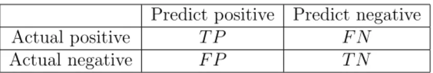
Table 3.2: Confusion matrix for a binary-class problem. Predict positive Predict negative Actual positive T P F N Actual negative F P T N
In the confusion matrix for a binary-class problem shown in Table 3.2, each of the com-ponents can be separately defined as:
True positive (T P): The number of positive individuals correctly predicted as positive.
False positive (F P): The number of negative individuals incorrectly predicted as pos-itive.
False negative (F N): The number of positive individuals incorrectly predicted as negative.
True negative (T N): The number of negative individuals correctly predicted as nega-tive.
com-ponents. True Positive Rate (TPR), also known as sensitivity or recall, measures the ratio of actual positives which are correctly identified. The formal definition of TPR is
TPR = T P
T P +F N (3.1)
False Positive Rate (FPR) measures the ratio of actual negatives which are incorrectly identified, which is formalized as:
F P R= F P
T N +F P (3.2)
The area under the ROC curve (AUC)[38] will be equal to 1 for an ideal model since
T P R = 1 and F P R = 0. AUC can be used to estimate the probability that a binary
classifier will give an arbitrary positive record a higher score than an arbitrary negative record, conditional on the assumption that the positive individual should receive a higher score than the negative one [39]. A random classifier’s AUC is 0.5; when AUC is higher than 0.5, the higher the AUC value, the better the prediction model [40].
3.2.2
MSE
The mean square error (MSE) is a good measure of how accurately the model predicts the outcome, and is one of the most important criterion for fit. Lower values of MSE indicate better fit. It is the estimation of the deviation between the observed outcome values and the predicted values in the form of
M SE= 1 n n X i=1 ( ˆf(xi)−yi)2 (3.3)
where ˆf(xi) and yi is the estimated outcome value and the actual outcome value for theith instance, respectively. From Eq. (3.3), we can see that MSE is the mean of the squared error shown in Eq. (2.11).
3.2.3
R
2The R2 [41] is used to measure the performance of regression models, which can be formalized as:
R2 = 1− RSS( ˆY)
V ar(Y) (3.4)
whereRSS( ˆY) is the residual sum of squares, andV ar(Y) is the variance of actual outcomes. For a dataset with n instances, these two terms can be mathematically defined as:
RSS( ˆY) = n X i=1 (yi−yˆi)2, andV ar(Y) = n X i=1 (yi−y¯)2 (3.5)
where ¯y is the mean value of the actual outcomes. For the ith instance, y
i is the actual outcome, and ˆyi = ˆf(xi) is the estimated outcome. According to Eq. (3.4), a good prediction model provides a small RSS( ˆY). In other words, the closer the R2 is to 1, the better the prediction will be [40].
3.3
Implementation Details
In this section, we explain our experimental setup used for evaluating the CRISP algo-rithm. The CRISP algorithm was implemented using the R programming language. All the machine learning models used for comparison in our work were also implemented in R. Elastic net was implemented using the glmnet R package for both the linear and logistic loss functions. Sparse Group Lasso (SGL) was implemented using the corresponding R package available in [42]. We implemented the hiernet-weak and hiernet-strong algorithms using the R package hierNet [21]. GAM and GA2M were implemented using the open source Java code available on github1, and in the implementation of GA2M model, only the top 50 inter-actions with lowest contribution to the overall error rate were considered for model building. We choose 50 as per the guidelines given in this paper [20]. L1- andL2- SVR correspond to theL2-regularized Support Vector Regression with theL1 andL2 loss functions, respectively. These were implemented using the LibLinear2 R package.
1
https://github.com/yinlou/mltk
2
We used the SPAMS3 package to implement the L
0 and L∞ models which are used to compare MSE and R2 values for all the three synthetic datasets. The performance results of all the models reported here are obtained using five-fold cross-validation. The model pa-rameters (λ, γ) are tuned over the validation data to reduce overfitting, and the evaluation results are based on the test data. The results and their corresponding standard deviation values are being reported. The R package pROC is used to calculate AUC values for all the models discussed in this thesis, and to calculate the MSE we used theMetrics4 package. We now describe the procedure we used to select λ and γ values which generate different candidate models in our CRISP algorithm. In our experiments, while doing the parameter tuning, we generated a sequence of values for the regularization parameter λ and the non-convexity parameter γ and selected the model corresponding to the optimal values (λ∗, γ∗) which were then used for prediction on the test data.
3.4
Goodness of Prediction
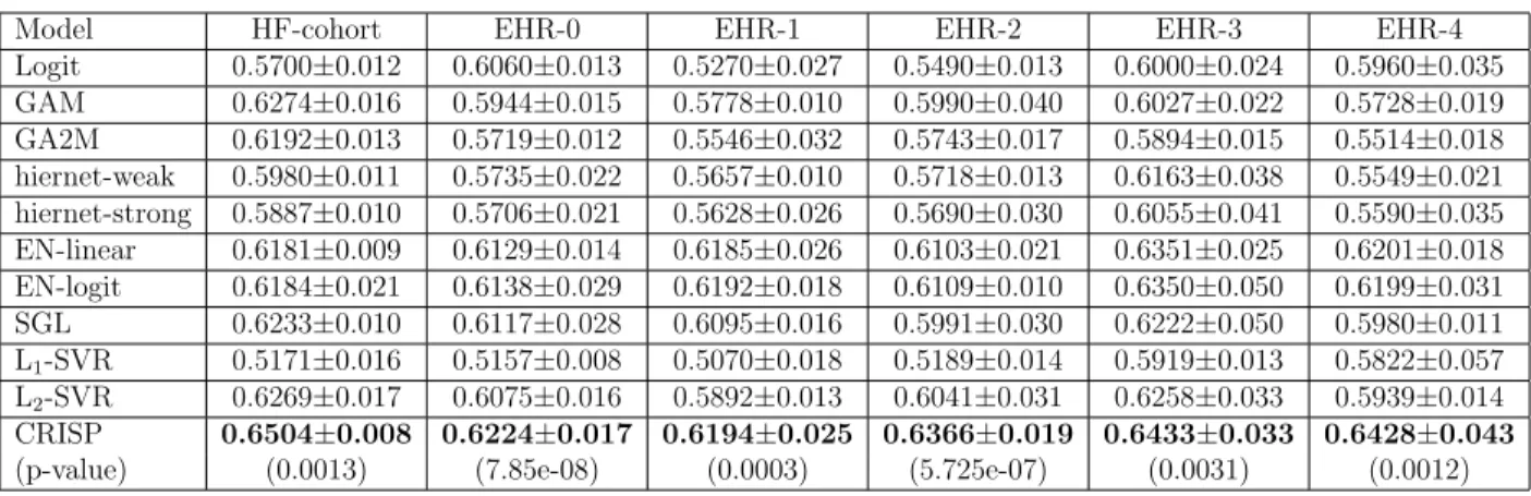
In this section, we compare the performance of CRISP with various competing models for the 30-day readmission problem on all the longitudinal EHRs. Table 3.3 summarizes the performance comparison results using AUC metric. The AUC values for CRISP algorithm in Table 3.3 are obtained from the optimal model parameters selected after applying the consensus criterion. For all of the datasets described in Table 3.1, our results for AUC evidently demonstrate that the proposed method CRISP provides significantly better results compared to the other methods. We also provide the P-values for CRISP to confirm the statistical significance of our results here. The P-value is calculated using Delong test method described in paper [43]. The null hypothesis is that the difference in AUC values between CRISP algorithm and the second best model is equal to zero. It should be noted that a result with a P-value of less than 0.05 is considered to be statistically significant and is interpreted as being small enough to justify the superiority over the methods used for comparison. Thus, these results given in Table 3.3 confirm that CRISP builds the most discriminative models
3
http://spams-devel.gforge.inria.fr/
4
Table 3.3: Performance comparison of CRISP with different models using AUC ± std for 30-day readmission problems on longitudinal EHRs.
Model HF-cohort EHR-0 EHR-1 EHR-2 EHR-3 EHR-4
Logit 0.5700±0.012 0.6060±0.013 0.5270±0.027 0.5490±0.013 0.6000±0.024 0.5960±0.035 GAM 0.6274±0.016 0.5944±0.015 0.5778±0.010 0.5990±0.040 0.6027±0.022 0.5728±0.019 GA2M 0.6192±0.013 0.5719±0.012 0.5546±0.032 0.5743±0.017 0.5894±0.015 0.5514±0.018 hiernet-weak 0.5980±0.011 0.5735±0.022 0.5657±0.010 0.5718±0.013 0.6163±0.038 0.5549±0.021 hiernet-strong 0.5887±0.010 0.5706±0.021 0.5628±0.026 0.5690±0.030 0.6055±0.041 0.5590±0.035 EN-linear 0.6181±0.009 0.6129±0.014 0.6185±0.026 0.6103±0.021 0.6351±0.025 0.6201±0.018 EN-logit 0.6184±0.021 0.6138±0.029 0.6192±0.018 0.6109±0.010 0.6350±0.050 0.6199±0.031 SGL 0.6233±0.010 0.6117±0.028 0.6095±0.016 0.5991±0.030 0.6222±0.050 0.5980±0.011 L1-SVR 0.5171±0.016 0.5157±0.008 0.5070±0.018 0.5189±0.014 0.5919±0.013 0.5822±0.057 L2-SVR 0.6269±0.017 0.6075±0.016 0.5892±0.013 0.6041±0.031 0.6258±0.033 0.5939±0.014 CRISP 0.6504±0.008 0.6224±0.017 0.6194±0.025 0.6366±0.019 0.6433±0.033 0.6428±0.043
(p-value) (0.0013) (7.85e-08) (0.0003) (5.725e-07) (0.0031) (0.0012) Table 3.4: Performance comparison of CRISP with machine learning models using MSE ±
std for the 30-day readmission problem on longitudinal EHRs.
Model HF-cohort EHR-0 EHR-1 EHR-2 EHR-3 EHR-4
Logit 0.2103±0.008 0.2056±0.004 0.2333±0.006 0.2254±0.010 0.2194±0.008 0.2283±0.011 GAM 0.1811±0.005 0.2122±0.010 0.2197±0.004 0.2246±0.009 0.2308±0.011 0.2488±0.014 GA2M 0.2238±0.010 0.2736±0.023 0.3154±0.048 0.3177±0.028 0.3089±0.038 0.3302±0.019 hiernet-weak 0.1914±0.008 0.2232±0.010 0.2226±0.002 0.2293±0.004 0.2309±0.010 0.2551±0.002 hiernet-strong 0.1933±0.007 0.2256±0.007 0.2297±0.005 0.2335±0.009 0.2250±0.008 0.2559±0.019 EN-linear 0.1832±0.003 0.2059±0.001 0.2075±0.002 0.2152±0.004 0.2145±0.004 0.2263±0.001 EN-logit 0.1833±0.006 0.2061±0.008 0.2077±0.009 0.2153±0.002 0.2146±0.004 0.2265±0.004 SGL 0.1816±0.003 0.2050±0.004 0.2065±0.008 0.2149±0.007 0.2151±0.009 0.2272±0.009 L1-SVR 0.7166±0.022 0.9585±0.037 0.9756±0.027 1.0635±0.041 1.0861±0.053 1.0814±0.107 L2-SVR 0.2402±0.007 0.2985±0.016 0.3104±0.026 0.3333±0.028 0.3441±0.049 0.3980±0.016 CRISP 0.1775±0.002 0.2030±0.003 0.2050±0.003 0.2110±0.003 0.2083±0.004 0.2202±0.003
compared to other methods. In Table 3.4, the mean squared error (MSE) along with the standard deviations for the 30-day readmission problem on all the datasets are provided. We observe that CRISP model outperforms all the other methods used in our comparisons. We can also observe that the standard deviation values of the results obtained from CRISP algorithm are significantly lower across all of the datasets compared to the other methods. This shows the robustness of our method.
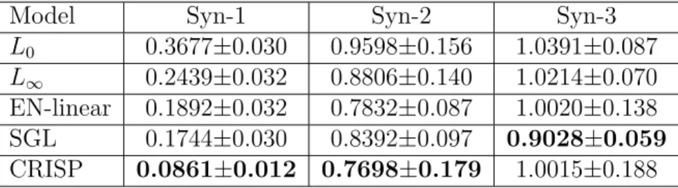
In Table 3.5 and Table 3.6, we show the MSE along with standard deviations and theR2 values for the three synthetic datasets using different regression models which are applicable to them. It can be observed that CRISP algorithm performs better when compared with other regression models using MSE and R2 on all the synthetic dataset except two cases: SGL method performs better with smaller MSE on Syn-3 and L∞ fits better than CRISP
Table 3.5: Performance comparison of CRISP with machine learning models using MSE ±
std on synthetic datasets.
Model Syn-1 Syn-2 Syn-3
L0 0.3677±0.030 0.9598±0.156 1.0391±0.087 L∞ 0.2439±0.032 0.8806±0.140 1.0214±0.070 EN-linear 0.1892±0.032 0.7832±0.087 1.0020±0.138 SGL 0.1744±0.030 0.8392±0.097 0.9028±0.059
CRISP 0.0861±0.012 0.7698±0.179 1.0015±0.188
Table 3.6: Performance comparison of CRISP with machine learning models using R2 on synthetic datasets.
Model Syn-1 Syn-2 Syn-3 L0 0.6269 0.1539 0.1602 L∞ 0.6197 0.2510 0.1269 EN-linear 0.8093 0.2064 0.1181 SGL 0.5046 0.1682 0.1038 CRISP 0.9124 0.2215 0.2057
with greater R2 on Syn-2. However, CRISP algorithm is the second best model in both cases. This better performance of our method is attributed to the fact that in addition to using a sparse and efficient non-convex regularizer within CRISP, the algorithm generates several candidate models, and then selects the best model using training data for prediction which gives a final model with good predictive ability.
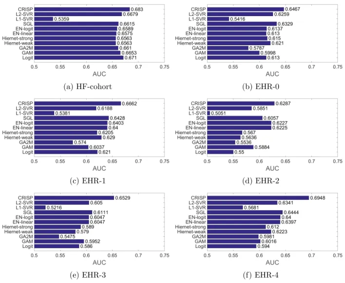
In Figure 3.2, we show the AUC values of CRISP model compared to other regression models using bar plots for the 365-day readmission problem on EHR datasets. One can observe that CRISP gives better performance compared to other regression models on all the EHRs.
(a) HF-cohort (b) EHR-0
(c) EHR-1 (d) EHR-2
(e) EHR-3 (f) EHR-4
Figure 3.2: Performance comparison of CRISP with various state-of-the-art methods for the 365-day readmission problem on longitudinal EHR datasets.
3.5
Scalability Experiments
In this section, we perform experiments to evaluate the scalability of the MC+ penalty which is used within CRISP along with other well known non-convex penalties mentioned in Table 1.1. We use the Matlab package called Generalized Iterative Shrinkage and Threshold-ing (GIST5) to fit these non-convex regularized linear regression models. These experiments were performed on a machine which has a main memory of 12 GB and a quadcore CPU.
5
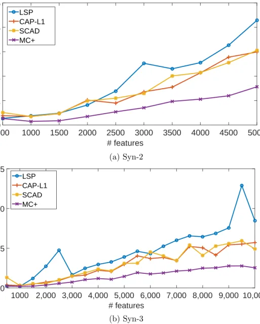
# features 500 1000 1500 2000 2500 3000 3500 4000 4500 5000 time (s) 0 1 2 3 4 5 LSP CAP-L1 SCAD MC+ (a) Syn-2 # features 1000 2,000 3,000 4,000 5,000 6,000 7,000 8,000 9,000 10,000 time (s) 0 5 10 15 LSP CAP-L1 SCAD MC+ (b) Syn-3
Figure 3.3: Comparison of time taken in seconds for three different non-convex regularizers compared to MC+ with increasing dimensionality of the features.
Two high-dimensional synthetic datasets, Syn-2 and Syn-3, described in Section 3.1.2 were used in this experiment. Figure 3.3 measures the computational time for the MC+ penalty compared to three competing non-convex regularizers. In this plot, the Y-axis represents the time taken in seconds which was averaged over five runs. The X-axis represents the dimensionality of the features.
based model runs faster compared to the other three models. LSP penalty based model takes highest time and the other two penalties, namely, SCAD and Capped `1 norm based models, are also slower than the MC+ penalty. Figure 3.3 (b) shows the scalability plot for Syn-3 dataset, and it can be observed that even in this case the MC+ penalty runs faster compared to the other models. This shows that our CRISP method which uses the MC+ penalty can perform efficiently on high-dimensional datasets.
3.6
Comparison with Clinical Models on EHRs
In this section, we conduct experiments to evaluate the clinical relevance of CRISP by comparing the performance of CRISP against four widely used clinical prediction models. Each of these models has been well studied in the clinical literature, therefore they serve as good baselines for comparison and evaluation. Our results demonstrate the superior performance of the CRISP algorithm.
3.6.1
Clinical Relevance
We now briefly introduce these four clinical models compared with the CRISP method.
• LACE [44]: This model assigns a score for each patient using the following risk factors: the length of stay (L), acuity of admission (A), comorbidity index score (C), and number of emergency hospital visits in six months before index admission (E).
• HOSPITAL [45]: This model assigns a score for each patient using the following risk factors: Oncology service information for each patient, sodium level, procedures dur-ing hospitalization, type of admission (planned or unplanned), number of admissions during 1 year before index hospitalization, and length of stay.
• Risk-o-Meter (ROM) [46]: This is a Bayesian method for risk prediction and it consists of two steps. Initially a clustering method is applied on the dataset and once we haveKclusters, the data will be partitioned intoK different datasets. Subsequently, a Naive Bayes classification algorithm is trained on allK datasets individually and each model will be evaluated.
• YALE [47]: This method uses a Hierarchical generalized linear model (HGLM) [48] based formulation. It includes a number of feature processing steps where only the patients with age ≥ 65 are considered. We include all the 154 clinically relevant features as determined by the study. These features include age, gender, 97 CCS, codes related to history of Percutaneous Coronary Intervention and history of Coronary Artery Bypass Graft. Once the pre-processing steps are done, we use a feature selection algorithm to determine important features. Finally, the accuracy of the model can be obtained by applying the HGLM method.
All the clinical models used in our performance comparison were also implemented in R. LACE [44] and HOSPITAL [45] models are score based, so for these models we only determine the risk score for each of the patients based on the values of the clinically relevant variables. Risk-o-meter (ROM) [46] was implemented using R, and the clustering in this algorithm was done using Nbclust. In Yale model [47], the dataset we use is obtained by considering only these patients with age ≥ 65 and the top 50 features selected using chi-squared feature selection method. Then the Hierarchical generalized linear model (HGLM) is applied on the filtered dataset to predict the risk.
Table 3.7 shows the AUC comparison of CRISP method with the four baseline clinical models on the HF-cohort dataset for both 30-day and 365-day readmission problems. It can be observed from this table that CRISP is performing better than all the other clinical models. The better performance of CRISP is attributed to its ensemble formulation and the non-convex regularized models being employed in the algorithm, which enables the method to have a good predictive ability.
3.6.2
Risk Calibration Plots
In this section, we study the goodness of fit of the proposed CRISP model using the risk calibration plots generated by the Hosmer-Lemeshow (HL) test statistic [49, 50]. Calibration plots are used to visualize the similarity between observed and predicted events, where predicted event risks are marked on X-axis and the observed event risks are marked on
Y-Table 3.7: AUC comparison of our approach with clinical models for 30-day and 365-day readmission problems on HF-cohort data.
Model 30-day 365-day LACE 0.5607 0.5307 HOSPITAL 0.5516 0.5206 YALE 0.6411 0.6762 ROM 0.5910 0.6240 CRISP 0.6504 0.6830
axis. If there is perfect agreement between observed and predicted rates, then all the points representing the corresponding subgroups should perfectly lie on the line drawn at 45◦.
0.0 0.2 0.4 0.6 0.8 1.0 0.0 0.2 0.4 0.6 0.8 1.0 Calibration plot Predicted risk Obser v ed r isk (a) 0.0 0.2 0.4 0.6 0.8 1.0 0.0 0.2 0.4 0.6 0.8 1.0 Calibration plot Predicted risk Obser v ed r isk (b)
Figure 3.4: Calibration plots for CRISP on HF-cohort data for (a) 30-day, (b) 365-day readmission problems.
Figure 3.4 shows the calibration plots for CRISP method on the HF-cohort dataset for both 30-day and 365-day readmission problems. It is intuitive that the predicted and observed risk values increase with time. However, we can observe from these plots that there is a strong agreement between the observed and predicted event rates both cases, which indicates that CRISP method is effective in predicting risks in the corresponding subgroups. We attribute this better performance to the non-convex regularized models used in the
CRISP algorithm and the consensus way of selecting the best model for prediction which gives a final model with good predictive ability.
CHAPTER 4
CONCLUSION AND FUTURE WORK
In this thesis, we presented a method called CRISP for solving the consensus regular-ization problem for regression which has not been addressed in the literature. This method generates a committee of non-convex regularized linear regression models using the minimax concave plus (MC+) penalty, and it applies a consensus criterion to select the best model for prediction. This method is effective because the problem of learning mutiple candidate models within the committee is solved using a generalized thresholding operator employed within a fast cyclic coordinate descent framework. We evaluated this model using longi-tudinal EHRs from a large hospital and high-dimensional synthetic datasets using diverse metrics such as AUC, MSE andR2. We also conducted experiments to assess the scalability of CRISP. Our results indicate that CRISP obtains higher AUC values compared to various other additive, interactions and sparse regression models. This work can be extended for solving an active learning regression model by querying the labels for an instance chosen after obtaining a consensus among multiple regularizers.
REFERENCES
[1] Ludmila I Kuncheva. A theoretical study on six classifier fusion strategies. IEEE Transactions on Pattern Analysis & Machine Intelligence, 24(2):281–286, 2002.
[2] Dymitr Ruta and Bogdan Gabrys. An overview of classifier fusion methods. Computing and Information systems, 7(1):1–10, 2000.
[3] Sergey Tulyakov, Stefan Jaeger, Venu Govindaraju, and David Doermann. Review of classifier combination methods. In Machine Learning in Document Analysis and Recognition, pages 361–386. Springer, 2008.
[4] Neal Parikh and Stephen P Boyd. Proximal algorithms. Foundations and Trends in optimization, 1(3):127–239, 2014.
[5] Laurent Condat. A generic proximal algorithm for convex optimizationapplication to total variation minimization. Signal Processing Letters, IEEE, 21(8):985–989, 2014. [6] David L Donoho and Jain M Johnstone. Ideal spatial adaptation by wavelet shrinkage.
Biometrika, 81(3):425–455, 1994.
[7] David L Donoho, Iain M Johnstone, G´erard Kerkyacharian, and Dominique Picard. Wavelet shrinkage: asymptopia? Journal of the Royal Statistical Society. Series B (Methodological), 57(2):301–369, 1995.
[8] Yiyuan She. Thresholding-based iterative selection procedures for model selection and shrinkage. Electronic Journal of statistics, 3:384–415, 2009.
[9] Gilles Gasso, Alain Rakotomamonjy, and St´ephane Canu. Recovering sparse signals with a certain family of nonconvex penalties and dc programming. Signal Processing, IEEE Transactions on, 57(12):4686–4698, 2009.
[10] Cun-Hui Zhang. Nearly unbiased variable selection under minimax concave penalty.
The Annals of statistics, 38(2):894–942, 2010.
[11] Pinghua Gong, Changshui Zhang, Zhaosong Lu, Jianhua Huang, and Jieping Ye. Gist: General iterative shrinkage and thresholding for non-convex sparse learning. Tsinghua University, 2013. http://www.public.asu.edu/ jye02/Software/GIST.
[12] Jianqing Fan and Runze Li. Variable selection via nonconcave penalized likelihood and its oracle properties.Journal of the American statistical Association, 96(456):1348–1360, 2001.
[13] Emmanuel J Candes, Michael B Wakin, and Stephen P Boyd. Enhancing sparsity by reweighted l1 minimization.Journal of Fourier analysis and applications, 14(5):877–905, 2008.
[14] Tong Zhang. Multi-stage convex relaxation for learning with sparse regularization. In D. Koller, D. Schuurmans, Y. Bengio, and L. Bottou, editors, Advances in Neural Information Processing Systems 21, pages 1929–1936. Curran Associates, Inc., 2009. [15] Pham Dinh Tao et al. The dc (difference of convex functions) programming and dca
revisited with dc models of real world nonconvex optimization problems. Annals of Operations Research, 133(1-4):23–46, 2005.
[16] Stephen Boyd, Neal Parikh, Eric Chu, Borja Peleato, and Jonathan Eckstein. Dis-tributed optimization and statistical learning via the alternating direction method of multipliers. Foundations and TrendsR in Machine Learning, 3(1):1–122, 2011.
[17] Yin Lou, Rich Caruana, and Johannes Gehrke. Intelligible models for classification and regression. In Proceedings of the 18th ACM SIGKDD international conference on Knowledge discovery and data mining, pages 150–158. ACM, 2012.
[18] Rich Caruana and Dayne Freitag. Greedy attribute selection. In ICML, pages 28–36. Citeseer, 1994.
[19] Rich Caruana, Yin Lou, Johannes Gehrke, Paul Koch, Marc Sturm, and Noemie El-hadad. Intelligible models for healthcare: Predicting pneumonia risk and hospital 30-day readmission. In Proceedings of the 21th ACM SIGKDD International Conference on Knowledge Discovery and Data Mining, pages 1721–1730. ACM, 2015.
[20] Yin Lou, Rich Caruana, Johannes Gehrke, and Giles Hooker. Accurate intelligible mod-els with pairwise interactions. In Proceedings of the 19th ACM SIGKDD international conference on Knowledge discovery and data mining, pages 623–631. ACM, 2013.
[21] Jacob Bien, Jonathan Taylor, and Robert Tibshirani. A lasso for hierarchical interac-tions. Annals of statistics, 41(3):1111–1141, 2013.
[22] Joseph Lee Rodgers and W Alan Nicewander. Thirteen ways to look at the correlation c