An application of copulas to improve PCA biplots for multivariate extremes

(1)

multivariate extremes

by

Justin Perrang

Research assignment presented in partial fulfilment of the

requirements for the degree of Master of Commerce

(Financial Risk Management) in the Faculty of Economic and

Management Sciences at Stellenbosch University

Supervisor: Mr. C.J. Van Der Merwe

(2)

DECLARATION

By submitting this research assignment electronically, I declare that the entirety of the work contained therein is my own, original work, that I am the sole author thereof (save to the extent explicitly otherwise stated), that reproduction and publication there of by Stellenbosch University will not infringe any third party rights and that I have not pre-viously in its entirety or in part submitted it for obtaining any qualification.

Signature:

Justin Perrang

Date:

(3)

ABSTRACT

Principal Component Analysis (PCA) biplots is a valuable means of visualising high di-mensional data. The application of PCA biplots over a wide variety of research areas containing multivariate data is well documented. However, the application of biplots to financial data is limited. This is partly due to PCA being an inadequate means of di-mension reduction for multivariate data that is subject to extremes. This implies that its application to financial data is greatly diminished since extreme observations are common in financial data. Hence, the purpose of this research is to develop a method to accommodate PCA biplots for multivariate data containing extreme observations. This is achieved by fitting an elliptical copula to the data and deriving a correlation matrix from the copula parameters. The copula parameters are estimated from only extreme observations and as such the derived correlation matrices contain the depen-dencies of extreme observations. Finally, applying PCA to such an “extremal” correla-tion matrix more efficiently preserves the relacorrela-tionships underlying the extremes and a more refined PCA biplot can be constructed.

(4)

Opsomming

Hoofkomponent Analise (HKA) bistippings is ’n nuttige metode om meer dimensionele data te visualiseer. Die toepassing van HKA bistippings is al goed gedokumenteer oor ’n wye verskeidenheid van navorsingsareas waar meerveranderlike data voorkom, maar die toepassing van bistippings op finansiële data is beperk. Dit is deels te wyte aan HKA wat ‘n onvoldoende metode is van dimensie reduksie van meerverander-like data wat ekstreme waarnemings bevat. Dit impliseer dat die toepassing daar-van op finansiële data aansienlik beperk is, gegee dat ekstreme waarnemings alge-meen voorkom in finansiële data. Die doel van hierdie navorsing is om ’n metode te ontwikkel om HKA- bistippings toe te pas op meerveranderlike data wat ekstreme waarnemings bevat. Dit word gedoen deur ’n elliptiese copula op die data te pas en ‘n korrelasiematriks uit die copula parameters af te lei. Die copula parameters word be-raam deur slegs die ekstreme waarnemings te gebruik en dus dui die afgeleide korre-lasiematrikse die afhanklikhede van slegs ekstreme waarnemings aan. Laastens, deur HKA op so ’n “ekstreme” korrelasie matriks toe te pas, word die verwantskappe on-derliggend aan die ekstreme waardes meer doeltreffend behou en kan ’n meer onder-skeidende HKA bistipping gekonstrueer word.

(5)

ACKNOWLEDGEMENTS

Firstly, I would like to acknowledge my supervisor, Carel van der Merwe, for his guid-ance and inspiration throughout my postgraduate studies. Your mentorship over the past few years has been invaluable. It was a pleasure learning from you!

Also, Professor T. De Wet, thank you for the time and effort you invested in guiding me during the year.

And, Professor W.J. Conradie, thank you for introducing me to the wonderful world of Financial Risk Management and for all the guidance you provided during my years at Stellenbosch University.

Furthermore, I would like to thank all the staff in the Department of Statistics and Ac-tuarial Science for all the support during my studies.

I would also like to extend my sincerest gratitude to...

Schroders Asset Management for funding my postgraduate studies.

My Parents, Gabriel and Elsabe, for their caring love, encouragement and support through-out my life.

My Girlfriend, Mighial Adams, for the love, support and, motivation through thick and thin.

My Classmates, Monique, Ryan, Jan, and Nadia, the last two years was a blast.

And Finally to my friends, Clay, Eaden, Jacques, Leonardo and Aldrin for the encour-agement and memories.

(6)

LIST OF FIGURES

2.1 Biplot for 95% VaR data. . . 12

2.2 Correlation biplot for 95% VaR data. . . 13

2.3 Biplot for 95% VaR data with predictions of day 16 VaR. . . 14

3.1 Simulation of 10000 bivariate normal andt4distributed random variables . 31

3.2 Scatter plot of univariate marginals corresponding to the Gaussian andt4

-Copula . . . 32

3.3 Scatter plots of univariate marginals corresponding to a Gumbel copula . . 36

3.4 Scatter plots of univariate marginals corresponding to a Clayton copula . . 36

3.5 Scatter plots of univariate marginals corresponding to a Frank copula . . . . 37

4.1 Flow diagram of the simulation structure . . . 47

5.1 Pairs scatter plot of a 5-variate Gamma-Gaussian distribution . . . 50

5.2 Traditional (a) and Refined (b) biplots for 5000 observations from a 5-variate Gamma-Gaussian distribution. . . 51

5.3 Pairs scatter plot of a 5-variate Gamma-Gumbel distribution . . . 56

5.4 Traditional (a) and Refined (b) biplots for 5000 observations from a 5-variate Gamma-Gumbel distribution. . . 57

(10)

5.6 Traditional (a) and Refined (b) biplots for 5000 observations from a 4-variate Heterogeneous-Gumbel distribution. . . 63

6.1 Pairs scatter plot for Rand/Foreign currency exchange rate monthly returns 68

6.2 Traditional biplot for Rand/Foreign currency exchange rate monthly returns 69

6.3 Refined biplot for Rand/Foreign currency exchange rate monthly returns . . 69

6.4 Traditional biplot prediction Rand/Foreign currency exchange rate monthly return on January 2016 . . . 72

6.5 Traditional biplot prediction Rand/Foreign currency exchange rate monthly return on January 2016 . . . 73

(11)

LIST OF TABLES

2.1 Van Blerk (2000) 95% VaR of financial trading desks . . . 11

2.2 Correlation matrix for 95% VaR of 7 financial trading desks . . . 14

2.3 Actual and predicted value of the 95% VaR for day 16 . . . 15

3.1 Popular families of Archimedean copulas . . . 34

5.1 Predictivity and Adequacy measures for biplots constructed from 5000 ob-servations from a 5-variate Gamma-Gaussian distribution. . . 52

5.2 Overall sample error for biplots constructed from 5000 observations from a 5-variate Gamma-Gaussian distribution. . . 52

5.3 Extreme sample error for biplots constructed from 5000 observations from a 5-variate Gamma-Gaussian distribution. . . 53

5.4 Overall and extreme sample error simulation results for biplots from a Gamma-Gaussian distribution. Each table consists of the average sample error, standard error and p-values for 4, 5 and 7 variables using 500 and 5000 observations for 20 and 80 tail samples. . . 54

5.5 Predictivity and Adequacy measures for biplots constructed from 5000 ob-servations from a 5-variate Gamma-Gumbel distribution. . . 57

5.6 Overall sample error for biplots constructed from 5000 observations from a 5-variate Gamma-Gumbel distribution. . . 58

(12)

5.7 Extreme sample error for biplots constructed from 5000 observations from a 5-variate Gamma-Gumbel distribution. . . 58

5.8 Overall and extreme sample error simulation results for biplots from a Gamma-Gumbel distribution. Each table consists of the average sample error, stan-dard error and p-values for 4, 5 and 7 variables using 500 and 5000 obser-vations for 20 and 80 tail samples. . . 60

5.9 Predictivity and Adequacy measures for biplots constructed from 5000 ob-servations from a 4-variate Heterogeneous-Gumbel distribution. . . 63

5.10 Overall sample error for biplots constructed from 5000 observations from a 4-variate Heterogeneous-Gumbel distribution. . . 64

5.11 Extreme sample error for biplots constructed from 5000 observations from a 4-variate Heterogeneous-Gumbel distribution. . . 64

5.12 Overall sample error simulation results for biplots from a 4-variate Heterogeneous-Gumbel distribution. The table constitutes the average sample error,

stan-dard error and p-values using 5000 observations and 80 tail samples. . . 65

5.13 Extreme sample error simulation results for biplots from a 4-variate Heterogeneous-Gumbel distribution. The table constitutes the average sample error,

stan-dard error and p-values using 5000 observations and 80 tail samples. . . 65

6.1 Predicitivity and Adequacy measures for biplots constructed using Rand/Foreign currency exchange rate monthly returns . . . 70

6.2 Average overall sample prediction error for Rand/Foreign currency exchange rate monthly returns . . . 70

6.3 Average extreme sample prediction error for Rand/Foreign currency ex-change rate monthly returns . . . 71

6.4 Prediction of Rand/Foreign currency exchange rate monthly return on Jan-uary 2016 . . . 73

(13)

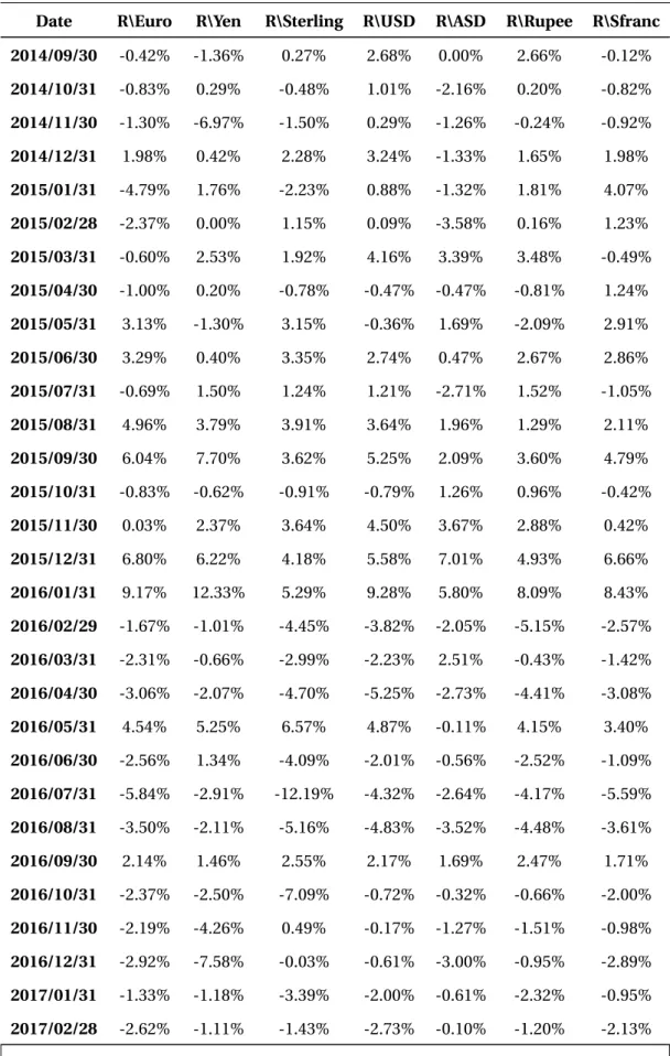
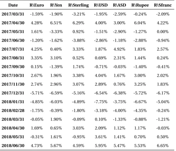
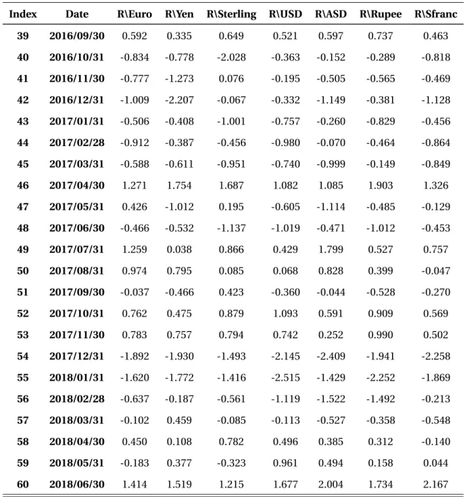
B.1 Rand foreign currency exchange rate monthly returns for period July 2013 to June 2018. . . 81

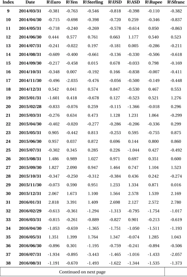
B.2 Standardised Rand foreign currency exchange rate monthly returns for pe-riod July 2013 to June 2018. . . 83

(14)

CHAPTER 1 INTRODUCTION

1.1 BACKGROUND AND MOTIVATION

In 1884, Abbott (1884) published a novel titledFlatland: A romance of many dimen-sions. In his novel Abbott (1884) attempted to challenge the notion of conceptualising higher dimensional space. To do this, he chronicles a tale of a square living in a 2-dimensional world known as Flatland. The novel unfolds when the square encounters a sphere living in 3-dimensional space. The sphere struggles to convince the square that he is not a circle, but an object in a higher dimension. The story of Flatland is an excellent thought experiment that demonstrates the difficulty of comprehending higher dimensions. Since humans can only visualise in 3 dimensions, our abilities are constrained when examining higher dimensional phenomena.

This limitation proves to be an obstacle in statistical analysis too, since in the words of Everitt (1994), “There are many patterns and relationships that are easier to discern in a graphical display than by any other data analysis method”. To overcome this hindrance, with regards to the visualisation of multivariate data for dimensions higher than three, Gabriel (1971) introduced the biplot. Biplots are a graphical technique constructed using dimension reduction techniques to visualise multivariate data in 2 or 3 dimen-sions. Note, however, that the “bi” in biplot does not refer to the dimensionality of the display, but due to a biplot displaying both observations and variables, simultaneously.

(15)

1.1. BACKGROUND AND MOTIVATION

The biplot was later extended by Gower and Hand (1996) to be used as a multivariate analogue of a scatter plot. There are many methods to construct biplots, however for the purpose of this study, only Principal Component Analysis (PCA) biplots are con-sidered. PCA is a methodology used to reduce the dimensionality of a dataset through identifying principal components, that preserve the maximum variation of the data, in lower dimensions. However, any form of dimension reduction will inevitably lead to a loss of information. This is true for PCA biplots too, however, the loss of information is compensated by the convenience of visualisation. The reason for only considering PCA in this study is twofold. Firstly, PCA is one of the simplest and widely applied dimension reduction techniques. Secondly, PCA and its related methods, such as fac-tor analysis, are widely applied and researched in the field of quantitative finance. In fact, one of the earliest published application of PCA was by Stone (1947), who applied PCA to economic time series data (Jolliffe, 2002). Since then PCA has been used in fi-nance both directly and indirectly, from modelling stock portfolios to analysing and constructing bond curves. Therefore, there is adequate justification that PCA biplots can be applied to visualise multivariate financial data.

Although PCA may be suitable in general for financial data, de Carvalho (2016) argues that PCA may be inappropriate if one’s purpose is to analyse the extremes of multi-variate data. This poses a problem for financial data since the extremes are essential to characterising risk, whereas the majority of the observations surrounding the mean is of less importance. Since PCA is an inadequate dimension reduction technique for multivariate extremes, it implies directly that PCA biplots may not be well suited for multivariate extremes. To overcome this, Chautruet al.(2015) proposes the use of clus-ter analysis combined with Principal Nested Spheres for dimension reduction of mul-tivariate extremes, but this does not allow for visualisation of the mulmul-tivariate dataset. The convenience and simplicity of PCA suggests that instead of abandoning PCA alto-gether, it may be useful to first experiment with adjusting PCA to be more appropriate for extremes. Such an adjustment can be pursued by considering alternative meth-ods to construct covariance and/or correlation matrices. The covariance matrix of a dataset is a critical part of PCA since the PCA methodology is based on preserving the maximum variation of a dataset. Similarly, if each variable in a multivariate dataset is

(16)

1.1. BACKGROUND AND MOTIVATION

scaled by its standard deviation and shifted to have a mean of zero, then the covariance and correlation matrix are the same. Hence, PCA can be executed on a correlation ma-trix of a scaled dataset. Jolliffe (2002) endorses PCA on a correlation mama-trix instead of a covariance matrix for two reasons. The first is that if variables are measured using different units, then PCA using a covariance matrix will be biased towards preserving the variable with the largest variation on its particular measurement scale. Secondly, it is more difficult to compare the results of PCA for different analyses when using the covariance matrix. However, the use of a covariance matrix does have its own advan-tages. The first being that if inference is the goal of statistical analysis then PCA on a covariance matrix is superior. Additionally, it is not possible to unscale PCA estimated data to represent the original data set when using the correlation matrix. Nonetheless, since the objective of PCA biplots is visualisation, PCA on the correlation matrix is used throughout this study to construct PCA biplots.

Owing to the fact that correlations will be used to perform PCA, the question is then how can the correlation matrix be adjusted to accommodate for multivariate extremes? It is firstly important to acknowledge that correlation is not the only way to measure dependence. Furthermore, correlation as a measure of dependence has the disadvan-tage of only measuring linear dependence. Moreover, Klüppelberg and Stelzer (2014) argues that in the context of risk one does not really care about correlation since the correlation depends on the whole distribution. Whereas, it is of more value in the risk management setting to find the dependence of extreme outcomes. Therefore a more rigorous approach to characterising dependence and more specifically extreme de-pendence is required. A possible solution is to consider copulas. According to Nelsen (2007), copulas are functions that join multivariate distribution functions from uni-variate marginal distribution functions. Given that copulas link variables, it therefore fully describes the dependence of the underlying variables in a multivariate distribu-tion. For this reason, this study will investigate how copulas can be used to construct correlation matrices. More specifically, the ability to construct a correlation matrix us-ing copulas for multivariate extreme observations. Given that multivariate extremes are the main concern, an appropriate dimension reduction technique would aim to preserve extremal dependencies instead of maximum variation. If a suitable

(17)

adjust-1.1. BACKGROUND AND MOTIVATION

ment for PCA is found to accommodate extremes, it will as a consequence, improve PCA biplots for multivariate extremes. An approach with this in mind was developed by Hauget al.(2015) who used an elliptical copula that is calibrated using the tail de-pendence function to construct a correlation matrix for multivariate extreme observa-tions. It can then be argued that performing PCA on a correlation matrix constructed from extremes should be more inclined to preserve extreme observations. Hence, an investigation into the application of such an extremal correlation matrix to construct PCA biplots is the primary objective of this study.

The study is performed by undertaking the following objectives:

1. A detailed discussion on the background and construction of PCA biplots.

2. Investigate the various PCA biplot quality measures.

3. Introduce the concept of dependence and various techniques to measure depen-dence.

4. Study in detail the development, use and properties of several copula families.

5. Demonstrate how elliptical copulas can be used to determine a correlation ma-trix for multivariate extremes.

6. Propose the use the derived correlation matrix for multivariate extremes, to im-prove PCA biplots for extreme observations.

7. Implement a simulation study to evaluate whether the proposed methodology improves PCA biplots for extreme observations.

8. Illustrate the suitability of the improved PCA biplot on real-world data that is subject to multivariate extremes.

To achieve the above-mentioned objectives this study is presented in the following se-quence:

InChapter 2 the necessary background for PCA biplots is discussed in detail. The chapter starts by firstly introducing the PCA methodology. This is followed by a

(18)

demon-1.1. BACKGROUND AND MOTIVATION

and interpretation of a PCA biplots are then illustrated. The chapter ends by providing some PCA biplot quality measures that are used to assess the overall fit of the biplot.

Chapter 3is dedicated to exploring the idea behind measuring dependence. It starts by introducing various dependence measures and discusses the purpose of each measure. The main component of this chapter is a review of copulas to measure dependence. This is done by discussing the theory underlying copulas as well as in-depth look into two copula families namely, the Elliptical and Archimedean copula families. It ends by reviewing a noteworthy application of copulas used to determine correlation matrices for multivariate extreme observations.

InChapter 4, the literature discussed in Chapter 2 and 3 is used to develop a method-ology to improve PCA biplots for extreme observations. This constitutes a discussion regarding the approach taken to improve PCA biplots as well as how such an improve-ment is evaluated.

InChapter 5, an empirical study by way of simulation is pursued, in order to deter-mine if the improved PCA biplot for extremes performs better than the traditional PCA biplots when assessing the fit of extreme values. This is done by simulating observa-tions from several multivariate distribuobserva-tions and examining the biplot fit at extremes for the improved and the traditional biplot methodology.

Chapter 6is a short chapter whereby the improved biplot methodology is tested against the traditional biplot methodology on a real-world financial dataset.

Finally, inChapter 7, the work carried out and contributions made are summarised and areas of further research are suggested.

(19)

CHAPTER 2 A REVIEW OF PCA BIPLOTS

As stated in the previous chapter, the use of PCA biplots (subsequently referred to as biplots) will be the focus of this chapter. The purpose of this chapter is to provide some needed background on the derivation and interpretation of biplots. Note that, some mathematical background required for this chapter is provided in Appendix A. Firstly, some background on PCA is given, then the use of PCA to construct biplots is discussed. This is followed by an explanation of how biplots can be interpreted by way of an example. The final section presents some useful techniques to measure the quality of a biplot display.

2.1 PRINCIPAL COMPONENT ANALYSIS (PCA)

PCA is one of the most popular dimension reduction techniques. The popularity of PCA is due to its simplicity and due to it being widely researched and applied in many fields of study. PCA originates from publications by Pearson (1901) and Hotelling (1933), who independently derived PCA using differing approaches. The differences in their approaches are owed to them having different motivations for their use of PCA. Pear-son (1901) was concerned with finding some lines and planes that best fit observations in ap-dimensional space. Hotelling (1933), on the other hand, wanted to determine observations ofpvariables by finding some smaller set of independent variables,

(20)

sim-2.1. PRINCIPAL COMPONENT ANALYSIS (PCA)

discussing PCA biplots, PCA will be viewed from the perspective of Pearson (1901).

The first step in PCA is to derive the principal components (PCs) of the underlying data matrix. PCs are derived by minimising the sum of the squared orthogonal distances (residuals) between the originalp-variable space and the reducedr-dimensional sub-space. Further, using the Huygens Principle, Gower and Hand (1996) proved that the optimalr-dimensional subspace is one that passes through the centroid of pointsX¯

in thep-variable space. This means that in order to optimally reduce ap-dimensional space to anr-dimensional space, the underlying observations X should be centred. Therefore, throughout this study, the assumption is made that an underlying data ma-trixX is preprocessed to be centred, i.e.E[X]=[µ1, ...,µp]0=[0, ..., 0].

SupposeX :n×pis a centred data matrix withpvariables andnobservations where the observation is denoted by the vectorxi,i =1, 2, ...,n. ThenX0X is proportional to

the sample covariance matrix ofX, which can be presented by applying Singular Value Decomposition (SVD)1as:

X0X =VΛV0 (2.1)

where,Λ:p×pis a diagonal matrix containing the ordered (from largest to smallest) eigenvalues ofX0X, denotedλi,i =1, 2, ...,p, andV :p×p is a matrix containing the

orthonormal eigenvectors ofX0X as its column vectors, ordered accordingly. Thep column vectors ofV denotedvi,i =1, 2, ...,pare termed the sample principal

compo-nents (Sample PCs). Further, the matrix of principal component scores (PC Scores),

Z :n×p, is determined as:

Z =X V (2.2)

which are coordinates of the sample PCs in thep-dimensional space.

To reduce the dimensionality of the data matrix tor-dimensional space the firstr col-umn vectors are extracted and denoted asVr :p×r. Thus,Vr is a matrix containing

the firstr eigenvectorsvi,i=1, 2, ...,r corresponding ther largest eigenvalues. It then

follows that the principal component approximation ofX is given by: ˆ

Z :n×p=X VrVr0 (2.3)

(21)

2.2. PCA BIPLOT CONSTRUCTION

this approximation yields the smallest sum of squared residuals between the original observations inp-dimensional spaces and its projection inr-dimensional space, i.e. ||X −Zˆ||2is minimised.

Alternatively, PCA can be performed by applying SVD directly on the data matrix X. The SVD ofX is given by:

X =UΩV0. (2.4)

SinceV is an orthogonal matrix, multiplying byV on the right of (2.4) yields,

X V =UΩ=Z (2.5)

which is the PC scores as in (2.2). To find ther-dimensional subspace the largestr singular values ofΩis extracted and denoted asΩr. Correspondingly, letUr andVr be

denoted as the firstr columns ofU andV, respectively. Then it follows that the best r-dimensional approximation of the data matrixX is given as:

X ≈X VrVr0=UrΩrVr0 (2.6)

The use of the derived sample PCs and PC scores to construct PCA biplots is discussed in the next section.

2.2 PCA BIPLOT CONSTRUCTION

As stated in Chapter 1, Gabriel (1971) introduced PCA biplots as a way to jointly repre-sent the observations and variables of a dataset. Then Gower and Hand (1996) adjusted the PCA biplot to represent a multivariate version of the traditional scatter plot which is used throughout this study. The construction of the PCA biplot is the focus of this section.

Gabriel (1971) states that the decomposition in (2.6) can also be represented as:

X ≈UrΩαrΩr1−αVr0=(UrΩαr)(Vr0Ωr1−α)0=GrHr (2.7)

withGr =UrΩαr,Hr0 =Vr0Ω1−r α, and 0≤α≤1. The purpose and use of a biplot display

(22)

2.2. PCA BIPLOT CONSTRUCTION

case forα=0 andα=1. Ifα=0, thenGr=Ur andHr0=ΩrVr sinceUr is orthonormal

the following can be derived:

X0X ≈(GrHr0)0(GrHr0)=HrGr0GrHr=HrHr. (2.8)

Therefore, entries inHr uniquely determine the covariance matrix ofX. Additionally,

it can be proven that whenα=0 the Mahalanobis distances are approximated between observations. Alternatively, ifα=1 thenGr =UrΩr andHr0=Vr0and it can be proven

in this case that the euclidean distances are approximated between observations. The differences between Mahalanobis2and euclidean distances is beyond the scope of this study. However, the choice ofα=1 will result in observations being represented better than variables on the biplot and ifα=0, it results in the variables, and as a conse-quence correlations, being represented better than the observations on the biplot. The PCA biplot of Gower and Hand (1996) assignsα=1, which is the assumption for the rest of this chapter. The biplot in the case whereα=0 is referred to as correlation biplot since variables are better represented.

In the previous section, it was shown that the bestr-dimensional subspace to repre-sent observations from ap-dimension space is determined by the firstr eigenvectors (Sample PCs) ofX0X denoted byVr. The columns ofVr provide a set of orthogonal

coordinate axes in ther-dimensional space termed the principal axes. The principal axes are used only for representing the biplot observations and is also referred to as the scaffolding axes. The biplot observations are determined as projections from the principal axes and are given by,

Zr=X Vr (2.9)

where, the rows ofZr represents the PC scores for the firstrsample PCs and is denoted

aszi:i =1, 2, ...,n.

The next step in the biplot construction is deciding whether the biplot will be used for interpolation or prediction. In the case of interpolation a newp-variable observation

x∗:p×1 has to be projected to an observation in ther-dimensional space asz∗:p×1.

2_{This is a generalised method to measure distance, introduced by Mahalanobis (1936). The}

Maha-lanobis distance measures the number of standard deviations a point is from the mean of its distribu-tion.

(23)

2.3. PCA BIPLOT INTERPRETATION

Thisr-dimension projection can be obtained using (2.9) as

z∗0=x∗0Vr (2.10)

Alternatively, in the case of prediction the originalp-variable observation must be ap-proximated asxˆ∗:p×1 from the coordinates in ther-dimensional spacez∗. This can be found using (2.6) as

ˆ

x∗=z∗0VrVr0 (2.11)

The choice between interpolation and prediction is not trivial since the biplot axes markers are different in both cases. Therefore, if the purpose of a biplot display is for both prediction and interpolation the two separate biplots must be constructed. How-ever, for the purposes of this study only predictive axes will be used.

The final step in biplot construction is plotting the axes that correspond to the p -variables of the data. As stated, axes for prediction and interpolation will differ in terms of the position of the axes markers. The different axes markers are determined by some value ofµ, with−∞ <µ< ∞. Supposeek:r×1 is a unit vector with thekt h element

equal to one and all other elements equal to zero. Then each observationxi with

coor-dinates (xi,1,xi,2, ...,xi,p) can be written as,

xi= p

X

k=1

xi,kek (2.12)

this will interpolate to the point,

z_i0=x_i0Vr= p

X

k=1

xi,kek0Vr (2.13)

Therefore thekt h interpolation biplot axis markers is determined byµekVr. It can

fur-ther be shown that the correspondingkt hprediction biplot axis markers is given by, µe_kVr

ekVrVr0e0_k

(2.14)

asµvaries.

2.3 PCA BIPLOT INTERPRETATION

(24)

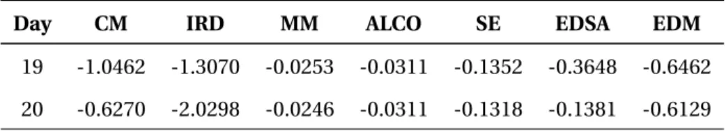
Van Blerk (2000) and further discussed in the textbook by Goweret al.(2011). The data used is daily 95% Value-at-Risk (VAR) observations for 7 financial trading desks over a 20 day period. The data used is provided in Table 2.1 and consists of 20 observations for 7 variables. Biplots are constructed throughout this study using the R packageUBbipl developed by le Roux and Lubbe (2013). The R code used to obtain the biplots and results presented below is given in Appendix C.1. The biplot for the 95% VaR dataset is illustrated in Figure 2.1. The axes in the biplot represent the variables which are the 95% VaR values for each of the 7 financial trading desks and the VaR observations for the portfolio are presented by the green points each labelled corresponding to the day of the measurement.

Table 2.1

Van Blerk (2000) 95% VaR of financial trading desks

Day CM IRD MM ALCO SE EDSA EDM

1 -1.7647 -0.2481 -0.2810 -0.2961 -0.1406 -0.2262 -0.9409 2 -0.8181 -1.3258 -0.2810 -0.2961 -0.1419 0.0123 -3.3836 3 -1.7152 -1.1400 -0.5961 -0.2961 -0.1410 -0.1825 -2.8719 4 -1.7714 -1.6412 -0.5961 -0.2961 -0.1454 -0.8900 -1.9459 5 -1.6613 -1.3016 -0.4124 -0.4755 -0.1319 -0.2153 -1.2899 6 0.0219 -1.3635 -0.6078 -0.2789 -0.2155 -0.2987 -1.3775 7 -0.8892 -1.1370 -0.4568 -0.4531 -0.1523 -0.2549 -1.1285 8 -0.9138 -1.1991 -0.4568 -0.4041 -0.1466 -0.0834 -1.1372 9 -1.1491 -1.1821 -0.4568 -0.4041 -0.1489 -0.3568 -1.1747 10 -1.2728 -0.7334 -0.4568 -0.4041 -0.1565 -0.5556 -0.8941 11 -0.8168 -0.8515 -0.4568 -0.4041 -0.1667 -0.3794 -0.8884 12 -1.2067 -1.5127 -0.4568 -0.4568 -0.1613 -0.0376 -0.8037 13 -0.8625 -1.8187 -0.4592 -0.4568 -0.1577 -0.1392 -0.9391 14 -2.5521 -1.4004 -0.4592 -0.4568 -0.1651 -0.1398 -0.9136 15 -1.4310 -1.3198 -0.4592 -0.4568 -0.1684 -0.1373 -1.0968 16 -2.8378 -1.3177 -0.4592 -0.4568 -0.1584 -0.3692 -0.1620 17 -1.0766 -1.2734 -0.7296 -0.4568 -0.2560 -0.0889 -1.1253 18 -1.0256 -1.3378 -0.7296 -0.4357 -0.2774 -0.2957 -1.0238

(25)

Table 2.1 – continued from previous page

Day CM IRD MM ALCO SE EDSA EDM

19 -1.0462 -1.3070 -0.0253 -0.0311 -0.1352 -0.3648 -0.6462 20 -0.6270 -2.0298 -0.0246 -0.0311 -0.1318 -0.1381 -0.6129 CM −3 −3 −2 −1 0 1 1 IRD −1.6 −1.4 −1.2 −1 MM −0.6 −0.5 −0.4 −0.3 ALCO −0.5 −0.5 −0.4 −0.3 −0.2 SE −0.2 −0.18 −0.16 −0.14 EDSA −0.4 −0.3 −0.2 −0.1 EDM −4 −3 −2 −1 0 1 2 3 4 5 6 78 9 10 11 12 13 14 15 16 17 18 19 20 Figure 2.1 Biplot for 95% VaR data.

The angles between biplot axes give an approximation of the correlation between vari-ables, where a small angle between axes indicates that variables are highly correlated and orthogonal axes indicate that observations have low correlation. However, the bi-plot constructed in Figure 2.1 takesα=1 as in (2.7), meaning that observations are better represented than variables. Conversely, in Figure 2.2 the correlation biplot is constructed withα=0, which better approximates the correlations between variables by the angles between axes since variables are better represented than observations.

(26)

When comparing Figures 2.1 and 2.2 with Table 2.2 providing the correlation matrix of the trading desk VaR values, it can be seen that neither biplot perfectly represents the correlation of the trading desks. However, Figure 2.2 does slightly better in represent-ing correlations, for example the angle betweenALCOandEDSAis slightly larger in Figure 2.2 to account for its low correlation.

CM −3 −3 −2 −1 0 IRD −1.4 −1.2 −1 MM −0.5 −0.4 −0.3 ALCO −0.5 −0.5 −0.4 −0.3 SE −0.18 −0.16 −0.14 EDSA −0.4 −0.3 −0.2 −0.1 EDM −3 −2 −1 0 1 2 3 4 5 6 78 9 10 11 12 13 14 15 16 17 18 19 20 Figure 2.2

(27)

Table 2.2

Correlation matrix for 95% VaR of 7 financial trading desks

CM IRD MM ALCO SE EDSA EDM

CM 1.00 -0.16 0.08 0.31 -0.23 0.18 -0.14 IRD -0.16 1.00 -0.08 -0.19 0.03 -0.11 -0.01 MM 0.08 -0.08 1.00 0.69 0.68 0.15 0.17 ALCO 0.31 -0.19 0.69 1.00 0.32 -0.13 -0.09 SE -0.23 0.03 0.68 0.32 1.00 -0.07 -0.12 EDSA 0.18 -0.11 0.15 -0.13 -0.07 1.00 -0.10 EDM -0.14 -0.01 0.17 -0.09 -0.12 -0.10 1.00 CM −3 −3 −2 −1 0 1 1 IRD −1.6 −1.4 −1.2 −1 MM −0.6 −0.5 −0.4 −0.3 ALCO −0.5 −0.5 −0.4 −0.3 −0.2 SE −0.2 −0.18 −0.16 −0.14 EDSA −0.4 −0.3 −0.2 −0.1 EDM −4 −3 −2 −1 0 1 2 3 4 5 6 78 9 10 11 12 13 14 15 16 17 18 19 20 Figure 2.3

(28)

2.4. PCA BIPLOT QUALITY MEASURES

Table 2.3

Actual and predicted value of the 95% VaR for day 16

CM IRD MM ALCO SE EDSA EDM

Actual -2.838 -1.318 -0.459 -0.457 -0.158 -0.369 -0.162 Predicted -2.803 -1.082 -0.447 -0.471 -0.151 -0.372 -0.156

To read off observations from the biplot, orthogonal lines are drawn from the observa-tion to each of the axes as illustrated in Figure 2.3, for the VaR sample on day 16. Since the biplot is a 2-dimensional approximation of observations in 7-dimensional space, there is a disparity between the actual observation values and those approximated on the biplot. The difference in the biplot approximation of the VaR on day 16 and its ac-tual value is presented in Table 2.3. Further, some variables are better approximated than others for example the discrepancy inIRDis large compared to the other instru-ments. Thus, given that a biplot is a visual approximation, measures of how well the biplot displays the underlying data are required and is discussed in the next section.

2.4 PCA BIPLOT QUALITY MEASURES

In the preceding sections, the construction and interpretation of a biplot were dis-cussed. However, the biplot interpretation is meaningless if the biplot does not display the data reasonably. Therefore, in this section, some biplot fit quality measures are ex-plored. The quality measures considered in this section are presented in more detail in the master’s thesis by Brand (2013).

Suppose throughout this section thatX is a centred data matrix whoseit hobservation is denoted asxi. Then from (2.6),X is approximated by,

ˆ

X =X VrVr0. (2.15)

The first measure of fit will be a measure of the overall quality of the biplot represen-tation denoted asV. The overall quality is determined as the ratio of the fitted sum of

(29)

2.4. PCA BIPLOT QUALITY MEASURES

squares and the total sum of squares as,

V =t r ace{Xˆ

0_X_ˆ_}

t r ace{X0_X_}. (2.16)

Now, (2.16) can be further simplified using (2.15) and (A.3) as:

V =t r ace{ ˆ X0Xˆ} t r ace{X0_X_} =t r ace{VrΩ 2 rVr0} t r ace{VΩ2_V0_} =t r ace{Ω 2 rVr0Vr} t r ace{Ω2_V0_V_} =t r ace{Ω 2 r} t r ace{Ω2_} = Pr i=1λi Pp i=1λi (2.17)

where,λi is theit h largest eigenvalue ofX0X. Given thatX0X is positive semi-definite

it implies thatλi ≥0,∀i thus 0≤V ≤1. Overall quality is at its maximum ifXˆ =X. It

is important to note that, even if the overall biplot quality is low, it can still be possible that some individual observations and variables are reasonably presented.

The next quality measure assesses how well the biplot axes represent the axes of the variables in thep-dimensional space which is termed the adequacy of the axes. The adequacy for the axis representing thekt h variable is denoted as γk and is given by Gardner-Lubbeet al.(2008) as γk = r X j=1 v2_{k j} (2.18)

where,v2_{k j} is thekt hrow and jt hcolumn entry of the matrixVrVr0.

Another quality measure proposed by Gardner-Lubbeet al.(2008) measures the pre-dictive ability of a biplots axes. The overall predictability of the biplots axes is expressed as:

Π=d i ag(Xˆ

0_Xˆ₎

d i ag(X0_X₎. (2.19)

Further, it can be shown that the predictivity of thekt hbiplot axis is given by,

πk= Pn i=1xˆ 2 i k Pn i=1x 2 i k . (2.20)

(30)

2.5. SUMMARY

biplot. Thus, high overall quality does not imply that axis predictivity is high for each of thepvariables.

The final biplot quality measure is presented by Brand (2013) and is termed the sam-ple predictivity. The samsam-ple predictivity measures the accuracy at which samsam-ples are approximated by the biplot. This implies that, if an observation has a low sample dictivity, then relative sample positions on the biplot is questionable. The sample pre-dictivity for theit hsample denoted asψi is expressed as,

ψi = ˆ x0 ixˆi x_i0xi . (2.21)

Similarly, the sample predictivity can also be evaluated for theit hsample as

ψ∗

i =(xˆi−xi)

2

. (2.22)

The sample prediction obtained using (2.22) will provide the sample prediction error for each variable and can be summed to find the overall sample predictivity.

All measures presented in this section are essential to the biplot display, as it presents a way to assess whether the biplot is a reasonable visualisation of the underlying data. Further, these measures should always be evaluated when a biplot is used since it pro-vides assurance as to whether the biplot representation is realistic.

2.5 SUMMARY

In this chapter, some necessary background on PCA and its application to construct biplots were provided. Further, an example of a biplot was presented accompanied by guidance on how to interpret biplots. Finally, some noteworthy methods to as-sess the quality of a biplot display was discussed. The next chapter will provide some background on dependence measures and copulas which are later used to improve the quality of a biplot.

(31)

CHAPTER 3 A REVIEW OF COPULAS AND

DEPENDENCE

An essential part of multivariate data analysis is to identify relationships between vari-ables, which is characterised by the underlying dependence between variables. The importance of dependence is extended by Jogdeo (1982) who noted, “Dependence re-lations between random variables is one of the most widely studied subject in prob-ability and statistics. The nature of dependence can take a variety of forms and un-less some specific assumptions are made about dependence, no meaningful statistical model can be contemplated”. In the previous chapter, linear correlation, as a measure of dependence, was used to perform PCA. This means that the concept of dependence is essential to PCA biplot construction. This chapter is therefore an examination of how to measure and interpret dependence as well as what underlying assumptions are required to characterise dependence. This chapter starts with some background on traditional measures of dependence. This is followed by a more modern look at de-pendence through the use of copula functions. Finally, this chapter is concluded by examining how to evaluate dependence for multivariate extremes.

(32)

3.1. DEPENDENCE MEASURES

3.1 DEPENDENCE MEASURES

In order to understand what it entails for variables to be dependent it is necessary to first define what it means for variables to be independent. Independence can be de-fined by considering a set ofdrandom variablesX1,X2, ...,Xd. Then this set of variables

are independent if and only if,

P(X1≤x1,X2≤x2, ...,Xd≤xd)=P(X1≤x1)P(X2≤x2)· · ·P(Xd ≤xd) (3.1)

If (3.1) does not hold it can be assumed that there exists some level of dependence between the underlying random variables. There are, however, many ways to measure dependence between variables and some of these dependence measures are discussed in this section.

The most well known and widely applied dependence measure is Pearson’s correlation coefficient (ρ), which is a measure of linear dependence between two random vari-ables. Suppose thatX,Y is a pair of random variables with some linear relationship. Then for these two variables,ρ(X,Y) can be calculated as,

ρ(X,Y)=p cov(X,Y)

v ar(X)v ar(Y), (3.2) with−1≤ρ(X,Y)≤1. IfX andY are independent thenρ(X,Y)=0. However, the con-verse does not hold, in other words,ρ(X,Y)=0 does not imply independence. Further, X andY have perfect linear dependence ifρ(X,Y)= ±1. The popularity of Pearson’s correlation coefficient as a measure of dependence is mainly due to it being easy to estimate from observed data. Additionally, Pearsons correlation serves as a natural de-pendence measure if data is distributed multivariate normally and as such, only in the case of multivariate normally distributed data doesρ=0 imply independence. How-ever, there are many disadvantages of Pearson’s correlations coefficient. The biggest disadvantage is that it only measures linear dependence and that it is not invariant under monotone transformations.1

The next measures of dependence that overcome some of the disadvantages of Pear-son’s correlation are measures of rank dependence or also referred to as ordinal

(33)

pendence. These dependence measures do not consider the magnitude of the obser-vations, but only the order of the observations. The first ordinal dependence measure discussed is Spearman’s correlation coefficient (ρS), which is sometimes also referred

to as Pearson’s correlation for ranked variables (Meissner, 2013). To defineρS, letX and

Y be continuous random variables with distribution functionsF1andF2, respectively.

Then Spearman’s correlation coefficient is given by,

ρS(X,Y)=ρ(F1(X),F2(Y)) (3.3)

whereρis Pearson’s correlation coefficient as in (3.2). SinceF1(X) andF2(Y) are

stan-dard uniform random variables the magnitudes ofX andY are irrelevant and thus only orders ofX andY are considered. Now, Klüppelberg and Stelzer (2014) states thatρS

can be calculated empirically as,

ˆ ρS(X,Y)= 1 2n(n 2 −1) n X i=1 · r ank(xi)− n+1 2 ¸· r ank(yi)− n+1 2 ¸ (3.4)

where,n is the number of observations and (r ank(xi),r ank(yi)) are the ranks of the

observations of (X,Y). Additionally,−1≤ρS ≤1 with the same interpretation as for

Pearson’s correlation.

The second ordinal dependence measure discussed was derived by Kendall (1938) and is known as Kendall’s tau (τ). Suppose that (X1,Y1) and (X2,Y2) are random vectors

with bivariate distribution functionF(X,Y). Then Kendall’s tau is given by,

τ(X,Y)=P[(X1−X2)(Y1−Y2)>0]−P[(X1−X2)(Y1−Y2)<0]. (3.5)

However, it is easier to grasp Kendall’s tau by considering its empirical version. The empirical formula for Kendall’s tau requires the definition of concordant and discor-dant observation pairs. The pair of observations (Xi,Yi) and (Xj,Yj) are said to be:

i. concordant, if bothXi >Xj andYi >Yj, or if bothXi<Xj andYi<Yj.

ii. discordant, ifXi>Xj andYi<Yj, or ifXi<Xj andYi >Yj.

(34)

The number of concordant and discordant pairs is then counted and the empirical Kendall’s tau is the calculated as,

ˆ

τ=(Number of concordant pairs)−(Number of discordant pairs)

Total number of pairs

= 2 n(n−1) X 1≤i≤j≤n si g n[(Xi−Xj)(Yi−Yj)] (3.6)

with,si g n=1 if observation pairs are concordant or si g n= −1 if observation pairs are discordant. When ˆτ=1 it implies that an increase inX always coincides with an increase inY and vice versa. The main advantage of ordinal dependence measures over linear dependence measures is that ordinal measures are invariant to monotone increasing transformations.

The final dependence measure discussed in this section pertains to a measure of de-pendence at multivariate extremes. Extreme dede-pendence is quantified through a tail dependence function. Naturally, a tail dependence function measures the dependency of the data in the tail. A tail dependence function distinguishes the dependency in the tail of the data to that of the regular data. Tail dependence is measured for a pair of random variables (X,Y) by determining if there is a non-zero probability thatX is large given thatY is large. Hence, random variables (X,Y) are said to be tail independent if

lim

t→∞P(Y >t|X >t)→0 (3.7)

Conversely, if the limit in (3.7) is non-zero then (X,Y) is said to be tail dependent. The tail dependence function characterises the strength of the dependence in the upper-and/or lower tail of a multivariate distribution. Therefore, it is not necessarily the case that the tail dependence in the upper- and lower tail of the distribution is identical and as such upper- and lower tail dependence is measured individually. The tail depen-dence function is defined by Klüppelberget al.(2007) as follows,

Definition 3.1(Tail dependence function). SupposeX =(X1, ...,Xd)0is a random vector

with distribution function F and continuous marginals F1, ...,Fd. Define the upper tail

dependence function ofX as λX upper(u1, ..,ud)= lim t→∞ 1 tP £ 1−F1(X1)≤t u1, ..., 1−Fd(Xd)≤t ud ¤ (3.8) with(u1, ..,ud)∈[0, 1]d.

(35)

3.2. COPULA THEORY

Similarly, define the lower tail dependence function ofX as, λX l ower(u1, ..,ud)=_tlim_→∞ 1 tP £ F1(X1)≤t u1, ...,Fd(Xd)≤t ud ¤ (3.9) with(u1, ..,ud)∈[0, 1]d.

Now,λ_{up per}X (1, 1, .., 1) is termed the upper tail dependence coefficient andλX_{l ower}(0, 0, .., 0)

is termed the lower tail dependence coefficient. Finally, Klüppelberget al.(2007) de-fines an empirical tail dependence function as follows:

Definition 3.2. SupposeX =(X1, ...,Xd)0is a random vector containing n samples, with

xh=(xh,1, ...,xh,d)0for h=1, ...,n, we define and empirical tail dependence function for

x>0as, λemp (x;k) := 1 k n X h=1 I ½ 1−Fj(xh,j)≤ k nxj ¾ j =1, ..,d (3.10) where1≤k ≤n and Fj denotes the empirical distribution function of Xj, j =1, ...,d .

Furthermore, define the empirical bivariate marginal tail dependence function as,

λemp_i_,_j (xi,xj;k) := 1 k n X h=1 I ½ 1−Fi(xh,i)≤ k nxi, 1−Fj(xh,j)≤ k nxj ¾ (3.11)

Since only tail events are considered k(n)→ ∞and k_n→0as n→ ∞.

There exist many more empirical tail dependence estimates for more detail see Schmidt and Stadtmüller (2006).

The next section deals with how, instead of empirical measures, functions known as copulas can be used to describe the dependence between random variables.

3.2 COPULA THEORY

A crucial element of multivariate statistics is describing the probability distribution of some random vector (X1, ...,Xd)0. The probability distribution function of (X1, ..,Xd)0is

characterised as follows:

(36)

3.2. COPULA THEORY

However, barring some well known multivariate distributions, expressingF(x1, ...,xd)

in (3.12) mathematically can be complex and be very specific to data with particu-lar attributes. A more convenient approach may be to consider the probability dis-tribution or marginal disdis-tributionFi(x) :=P(Xi <x) of each of the random variables

Xi,i =1, 2, ...,d individually. Then once each random variable can be described by

some known marginal distribution, combining these marginals to a multivariate dis-tribution can then be pursued. Thus in addition to the description of the marginal distribution for each variable, a function is required to combine these marginals in a mathematically sound manner. Furthermore, such a function would not only combine these marginal distributions but as a consequence also fully describe the dependence between the random variables. A function that constructs a multivariate distribution from underlying marginal distributions is known as a copula. The word copula origi-nates from Latin to mean “a link, tie or bond”(Nelsen, 2007).

Copulas was first described by Sklar (1959) as a function that joins one-dimensional probability distributions to form multivariate probability distributions. Further, he de-tailed a theorem which is now considered to be the fundamental theorem in the field of copulas and as such it is termed Sklar’s Theorem.

Theorem 3.1(Sklar’s Theorem). A function F :Rd →[0, 1]is the distribution function of some random vector(X1, ...,Xd)0if and only if there is a copula C : [0, 1]d →[0, 1]and

univariate distribution functions F1, ...,Fd:R→[0, 1]such that

C(F1(x), ...,Fd(x))=F(x1, ...,xd), x1, ...,xd ∈R (3.13)

If marginals F1, ...,Fd are continuous, then C is unique. Conversely, if C is a copula and

F1, ...,Fd are univariate distribution functions, then the function F defined in (3.13) is a

joint distribution function with margins F1, ...,Fd.

Similarly, Sklar’s Theorem can be applied to construct multivariate survival functions. A survival function of a random vector (X1, ...,Xd)0is defined as

¯

F(x1, ...,xd)=P(X1>x1, ...,Xd>xd), x1, ...,xd∈R (3.14)

Each random variable is specified by its marginal survival function ¯Fj(x) :=P(Xj >

(37)

3.2. COPULA THEORY

the marginal survival functions a survival copula ˆC is employed. Furthermore, Sklar’s Theorem can be reformulated for survival copulas as follows.

Theorem 3.2(Sklar’s Theorem for Survival Functions). A functionF¯:Rd →[0, 1]is the distribution function of some random vector(X1, ...,Xd)0if and only if there is a survival

copulaCˆ : [0, 1]d →[0, 1]and univariate survival functions F¯1, ..., ¯Fd :R→[0, 1]such

that

ˆ

C(F1(x), ...,Fd(x))=F¯(x1, ...,xd), x1, ...,xd ∈R (3.15)

If marginalsF¯1, ..., ¯Fd are continuous, thenC is unique. Conversely, ifˆ C is a survivalˆ

copula andF¯1, ..., ¯Fd are univariate survival functions, then the function F defined in¯

(3.15) is a joint survival function with marginsF¯1, ..., ¯Fd.

Since the publication of Sklar’s Theorem, copulas have been applied over a wide variety of fields. Copulas was especially applied in the field of finance and according to Salmon (2012) is partly to blame for the 2008/9 credit crises. A more thorough mathematical examination of copulas can be found in Nelsen (2007).

As stated earlier, since a copula combines the marginals of all random variables it, as a consequence, also fully describes the dependence between all random variables. Therefore, copulas can be used not only to construct multivariate distributions, but also to analyse the dependence in a multivariate dataset. Given that the topic of this study is to apply alternative dependence measures to biplots, copulas will be studied for its ability to characterise dependence. If a copula fully characterises dependence then it is obvious that a copula should, to an extent, be associated with alternative de-pendence measures such as Kendall’s tau and Spearman’s rho, which is described by Nelsen (2007) in the following theorems.

Theorem 3.3(Kendall’s tau Copula Specification). Let X and Y be continuous ran-dom variables whose copula is C . Further, let FX and FY be the respective marginal

distribution functions and define a random vector of uniform variables by(U,V) := [FX(X),FY(Y)]. Then Kendall’s tau for X and Y is given by

τX,Y =τC :=4 Z 1 0 Z 1 0 C(u,v)dC(u,v)−1=4E[C(U,V)]−1 (3.16)

(38)

3.2. COPULA THEORY

Theorem 3.4(Spearmans rho Copula Specification). Let X and Y be continuous ran-dom variables whose copula is C . Further, let FX and FY be the respective marginal

distribution functions and define a random vector of uniform variables by(U,V) := [FX(X),FY(Y)]. Then Kendall’s tau for X and Y is given by

ρX,Y =ρC:=12 Z 1 0 Z 1 0 C(u,v)dudv−3 (3.17)

The relationships described in Theorems 3.3 and 3.4 are useful when fitting a copula to a dataset. Given that Kendall’s tau and Spearmans rho are easy to estimate from ob-servations, the relationships above can be used to estimate the parameters for a para-metric copula.

Finally, it is further shown by Nelsen (2007) that the tail dependence coefficient de-pends solely on the underlying copula of a multivariate distribution. This is conveyed by the following theorem.

Theorem 3.5. Let X and Y be continuous random variables whose copula is C . Further, let FX and FY be the respective marginal distribution functions and define a random

vector of uniform variables by(U,V) :=[FX(X),FY(Y)]. Then the upper- and lower-tail

dependence coefficients for X and Y is given by

λupper(U,V) :=lim t→1 C(t,t)−2t+1 1−t (3.18) and λl ower(U,V) :=lim t→0 C(t,t) t (3.19)

Given that estimating the tail dependence coefficients is challenging since is entails estimating a property in a limit from finite observations, it is simpler to first fit a copula to the data and then use the relationship in Theorem 3.5 to determine the upper- and lower-tail dependence coefficients.

In the subsequent section, some popular copula families and their properties are ex-amined.

(39)

3.2. COPULA THEORY

3.2.1 Elliptical copulas

One of the central themes of this study is to find a method to characterise extreme de-pendence. To achieve this, properties from an elliptical copula will be applied. There-fore, this section is devoted to presenting the necessary background on elliptical cop-ulas.

Before elliptical copulas can be discussed it is first necessary to ask:What is an ellip-tical distribution ? The family of elliptical distributions consists of distributions that generalise the multivariate normal distribution, for example the multivariate Student-t disStudent-tribuStudent-tion. An ellipStudent-tical disStudent-tribuStudent-tion is consStudent-trucStudent-ted by combining ellipStudent-tical marginal distributions through an elliptical copula. More generally, an elliptical distribution can be obtained through a linear transformation of a spherical distribution. A spherical distribution is defined as follows:

Definition 3.3(Spherical distribution). Suppose thatO:d×d is an orthogonal matrix such thatO0O=I . Then a d -dimensional random vectorX =(X1, ...,Xd)0has a spherical

distribution if for every matrixOone has

OX =d X (3.20)

Equivalently, there exists a random variable R≥0and ,independently, a d -dimensional random vectorSwith a uniform distribution on an unit sphere, such that

X =d RS. (3.21)

Furthermore, a spherical distribution is fully described through a functionφ: [0,∞)→

R, referred to as a characteristic or generator function ofX. Hence, the distribution of ad-dimensional spherical random variable is denoted asX _vSd(φ). Since an elliptical

distribution is merely a linear transformation of a spherical distribution the following theorem holds.

(40)

distribu-3.2. COPULA THEORY

d -dimensional random vector on a unit hypersphere, and a d×k matrixAwithA A0=Σ, such that

Z =d µ+A0X =d µ+RA0S (3.22)

withX _vSd(φ).

From Theorem 3.6 the definition of an elliptical distribution follows directly.

Definition 3.4(Elliptical distribution). IfZ is a d -dimensional random vector and, for some vectorµ∈Rd, some d×d non-negative definite symmetric matrixΣ, and some functionφ: [0,∞)→R, the characteristic functionϕZ−µofZ−µis of the formϕZ−µ(t)= φ(t0Σt), we say that Z has an elliptical distribution with parametersµ, Σandφ, and

we writeZ _vEd(µ,Σ,φ).

Further, Klüppelberg and Kuhn (2009) proves that ifZ_vEd(µ,Σ,φ) is transformed as,

Z∗:=d i ag(σ11, ...,σd d)

1

2Z (3.23)

thenZ∗_vEd(µ,R,φ) withR:=(σi j/pσi iσj j)i≤j,j≤dthe correlation matrix ofZ. Hence

under a suitable transformation an elliptical copula can be specified via its correlation matrix and characteristic functionφ.

The correlation matrix from an elliptical distribution has a useful relationship with Kendall’s tau, which is presented in Theorem 3.7.

Theorem 3.7. LetZ _vEd(µ,R,φ), where for i,j ∈1, 2, ...,d , Zi and Zj are continuous

with correlation coefficientρi j. Then,

τ(Zi,Zj)=

2

πarcsinρi j. (3.24)

This relationship can be used to find for the correlation coefficientρi j by estimating

τ(Zi,Zj) and inverting (3.24).

Before the extremal dependence properties of an elliptical distribution can be exam-ined, it is first necessary to define the concept of a regularly varying random variable. A regularly varying random variable is defined as follows:

(41)

3.2. COPULA THEORY

Definition 3.5(Regular variation). A random variable R is said to be regularly varying with indexα>0if for all x>0,

lim

t→∞

P(R>t x) P(R>t) =x

−α _(3.25)

A regularly varying random variable is merely a random variable whose tail behaviour is similar to that of a power law function. According to Hult and Lindskog (2002) the concept of regular variation is connected to the tail dependence function of an ellipti-cal distribution in the following theorem.

Theorem 3.8. LetZ =d µ+RA0S_vEd(µ,Σ,φ)withΣi i >0for i =1, 2, ...,d ,|ρi j| <1for

all i6=j , and whereµ, R,AandS are as in Theorem 3.6. Then the following statements are equivalent:

i. R is regularly varying with indexα>0.

ii. Z is regularly varying with indexα>0.

iii. For all i6=j ,(Zi,Zj)has tail dependence coefficient

λU(Zi,Zj)=λ`(Zi,Zj)= Rπ/2 (π/2−arcsinρi j)/2cos α₍_t_)d_t Rπ/2 0 cosα(t)dt . (3.26)

Hult and Lindskog (2002) concludes from Theorem 3.8 that an elliptically distributed random vectorZ will only have tail dependence if the random variableR inZ =d µ+

RA0S is regularly varying. Moreover, the correlation coefficientρi j only affects the

magnitude of the tail dependence. This consequently implies that a bivariate obser-vation (Zi,Zj) can have a large tail dependence coefficient even if its correlation

coef-ficient is zero.

A more generalised approach to characterise the dependence for an elliptical distribu-tion is through an elliptical copula which is defined as follows.

Definition 3.6(Elliptical copula). An elliptical copula is defined as the copula related to an elliptical distribution F , and is obtained using Sklar’s theorem as,

C(u1, ...,ud)=F £ F₁−1(u1), ...,F_d−1(ud) ¤ , u1, ...,ud ∈[0, 1]d (3.27) 1

(42)

3.2. COPULA THEORY

Two of the most well known elliptical distributions is the multivariate- normal and Student-t distributions, both having corresponding elliptical copulas defined as fol-lows:

Definition 3.7(Gaussian copula). The Gaussian copula CGuass_R is the copula of X _v

Nd(0,R), whereRis the correlation matrix ofX. The analytical form is given by

CGuass_R :=ΦR£Φ−1(u1), ...,Φ−1(ud)

¤

(3.28)

where(u1, ...,ud)∈[0, 1]d,ΦRis the joint distribution function ofX, andΦ−1is the

quan-tile function of the standard normal distribution.

Definition 3.8(t-Copula). The t -Copula C_Rt _,_νis the copula ofX _vtd(0,R,ν), whereR

is the correlation matrix ofX. The analytical form is given by C_Rt _,_ν:=t_ν,R

£

t_ν−1(u1), ...,t_ν−1(ud)

¤

(3.29)

where(u1, ...,ud)∈[0, 1]d,tν,Ris the joint distribution function ofX, and t_ν−1is the quan-tile function of the Student-t distribution withνdegrees of freedom.

Further, the upper and lower tail dependence of the Gaussian copula is zero, i.e the Gaussian copula is tail independent. However, for thet-Copula the upper and lower tail dependence is identical and is expressed as

λU(Xi,Xj)=λ`(Xi,Xj)=2tν+1 µ − s (ν+1)(1−ρi j) 1+ρi j ¶ (3.30)

withνthe degrees of freedom.

Algorithms 3.1 and 3.2, as given by Embrechtset al.(2002), provides the steps to gen-erate multivariate samples using the Gaussian and t-Copula, respectively.

Algorithm 3.1(Simulatingnmultivariate samples from the Gaussian copula). In order to generate n observations from a d -variate distribution with marginal distributions F1,F2, ...,Fd and quantile functions F1−1,F2−1, ...,Fd−1that is specified and known.

Addi-tionally, suppose that dependence structure is characterised by a Gaussian copula with correlation matrixR. Then perform the following steps:

An application of copulas to improve PCA biplots for multivariate extremes

multivariate extremes

by

Justin Perrang

Research assignment presented in partial fulfilment of the

requirements for the degree of Master of Commerce

(Financial Risk Management) in the Faculty of Economic and

Management Sciences at Stellenbosch University

DECLARATION

ABSTRACT

Opsomming

ACKNOWLEDGEMENTS

CONTENTS

LIST OF FIGURES

LIST OF TABLES

CHAPTER 1

INTRODUCTION

1.1 BACKGROUND AND MOTIVATION

CHAPTER 2

A REVIEW OF PCA BIPLOTS

2.1 PRINCIPAL COMPONENT ANALYSIS (PCA)

2.2 PCA BIPLOT CONSTRUCTION

2.3 PCA BIPLOT INTERPRETATION

2.4 PCA BIPLOT QUALITY MEASURES

2.5 SUMMARY

CHAPTER 3

A REVIEW OF COPULAS AND

DEPENDENCE

3.1 DEPENDENCE MEASURES

3.2 COPULA THEORY

3.2.1 Elliptical copulas