Graphlet Correlations for Network Comparison and Modelling: World Trade Network Example

Imperial College London Department of Computing

Graphlet Correlations for Network

Comparison and Modelling: World

Trade Network Example

¨

Omer Nebil Yavero˜glu

December 2013

Submitted in part fulfilment of the requirements for the degree of Doctor of Philosophy in Computing of Imperial College London

Declaration

I herewith certify that all material in this dissertation which is not my own work has been properly acknowledged.

¨

Omer Nebil Yavero˜glu

Copyright

The copyright of this thesis rests with the author and is made available under a Creative Commons Attribution Non-Commercial No Derivatives licence. Researchers are free to copy, distribute or transmit the thesis on the condition that they attribute it, that they do not use it for commercial purposes and that they do not alter, transform or build upon it. For any reuse or redistribution, researchers must make clear to others the licence terms of this work.

Abstract

We propose methods on two fundamental graph theoretic problems: (1) network comparison, and (2) network modelling. Our methods are applied to five real-world network types, with an emphasis on world trade networks (WTNs), which we choose due to the world’s current economic crisis.

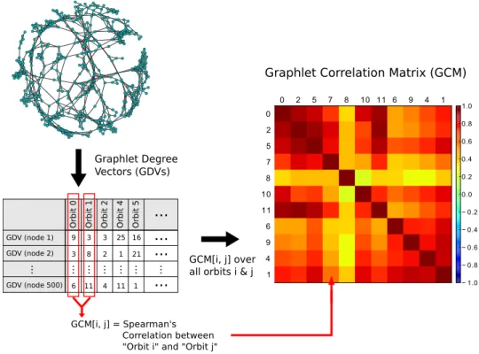
Finding topological similarities of complex networks is computationally intractable due to NP-Completeness of the subgraph isomorphism problem. Hence, simple heuristics have been used for this purpose. The most sophis-ticated heuristics are based on graph spectra and small subnetworks includ-ing graphlets. Among these, graphlets are preferred since spectra do not provide a direct real-world interpretation of network structure. However, current based techniques can be improved. We improve graphlet-based heuristics by defining a new network topology descriptor, Graphlet Correlation Matrix (GCM), which eliminates all redundancies and quan-tifies the dependencies in graphlet properties. Then, we introduce a new network distance measure,Graphlet Correlation Distance (GCD), that com-pares GCMs of two networks. We show that GCD has the best network classification performance, is highly noise-tolerant, and is computationally efficient. Using this methodology, we highlight a three-layer organization in the WTNs: core, broker, and periphery. Furthermore, we uncover the link between the dynamic changes in oil price and trade network topology.

Network models should shed light on the rules governing the formation of real networks. Using GCD, we identify models that fit five real-world network types. However, none of these standard network models fit WTNs. Hence, we introduce two new network models: one that mimics the Gravity Model of Trade, and the other that mimics brokerage / peripheral position-ing of a country in WTN. Also, we show that economic wealth indicators of a country are predictive of its future brokerage position. Finally, we use exponential-family random graph modelling approach to build a generic framework that enables modelling based on any graphlet property.

To my parents, family and friends...

None of this would have been possible without your

precious support.

Acknowledgements

I am grateful to my supervisor, Professor Nataˇsa Prˇzulj, for her guidance and support on my research. Prof. Prˇzulj’s enthusiasm on always targeting higher motivated me to be more productive in this study, and gain a lot more than I expected from my studies. Prof. Prˇzulj’s experience in research also helped me to develop skills required for being an independent researcher.

I would like to thank my examination committee members, Prof. Duncan F. Gillies and Prof. Desmond Higham, for their time and insightful feedback on this dissertation. I also want to thank my second supervisor, Prof. Marek Sergot, for his helpful mentoring throughout my studies.

I am grateful to all the past and present members of Prof. Prˇzulj’s re-search group: Dr. No¨el Malod-Dognin, Dr. Joana Gon¸calves, Kai Sun, Anida Sarajlic, Vuk Janjic, Miles Mulholland, and Yulian Ng. Apart from your scientific contribution to my work with our discussions, your friendship and support has been very valuable to me over the years.

I want to thank Dr. Aleksandar Stojmirovic for initiating great ideas for my studies, and also for guiding the implementation of these ideas with his insightful discussions. Our collaborators did not only help us develop excellent ideas, but also made our research more exciting and dynamic by supplying us with new ideas from di↵erent disciplines. I sincerely thank Prof. Athina Markopoulou, Prof. Carter Butts, Dr. Maciej Kurant, Sean M. Fitzhugh, Darren Davis, Prof. Rasa Karapandza, and Prof. Zoran Levnajic for their collaboration.

I would like to acknowledge Prof. Sinan Kalkan and Hande C¸ elikkanat for their patience and e↵ort in proof-reading this dissertation.

I am extremely grateful to my family, whom not only supported me by all means during my studies but also encouraged me to chase my dreams at the expense of being far away from me.

Finally, I would like to thank to Imperial College London – Department of Computing, European Research Council (ERC) Starting Independent

Re-searcher Grant 278212 (2012-2017), and USA National Science Foundation (NSF) Cyber-Enabled Discovery and Innovation (CDI) grant OIA-1028394 for funding my studies.

Contents

1.4 Introduction to Network Comparison . . . 40

1.5 Introduction to Network Modelling . . . 44

1.5.1 Random Network Models . . . 45

1.5.2 Exponential-family Random Graph Models . . . 48

1.5.3 Evaluating Model Fit on Real-World Networks . . . . 52

1.6 Previous Studies on World Trade Networks . . . 56

1.7 Dissertation Outline . . . 58

2 Network Analysis & Comparison: Graphlet Correlations Approach 61 2.1 Motivation . . . 61

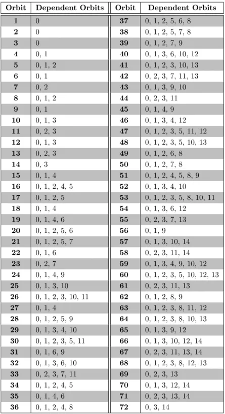
2.2 Redundancies and Dependencies in Graphlet Degree Vectors . 62 2.3 Graphlet Correlations . . . 67

2.3.1 Graphlet Correlation Matrix . . . 69

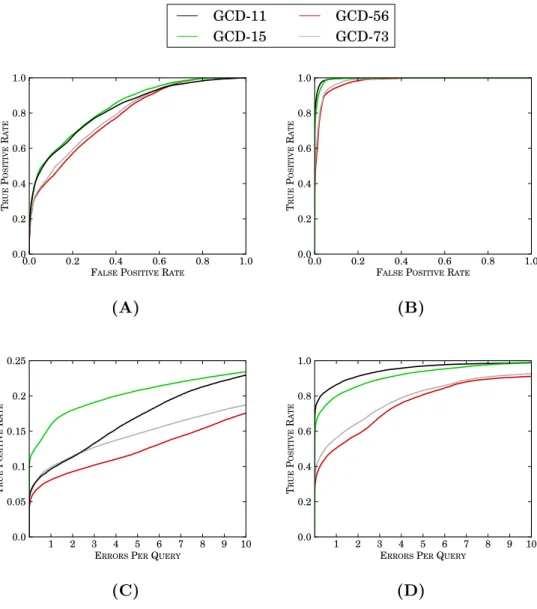
2.3.2 Graphlet Correlation Distance . . . 73

2.4 Validation Results . . . 74

2.4.1 Performance on Model Clustering . . . 74

2.4.2 Performance on Noisy Networks . . . 85

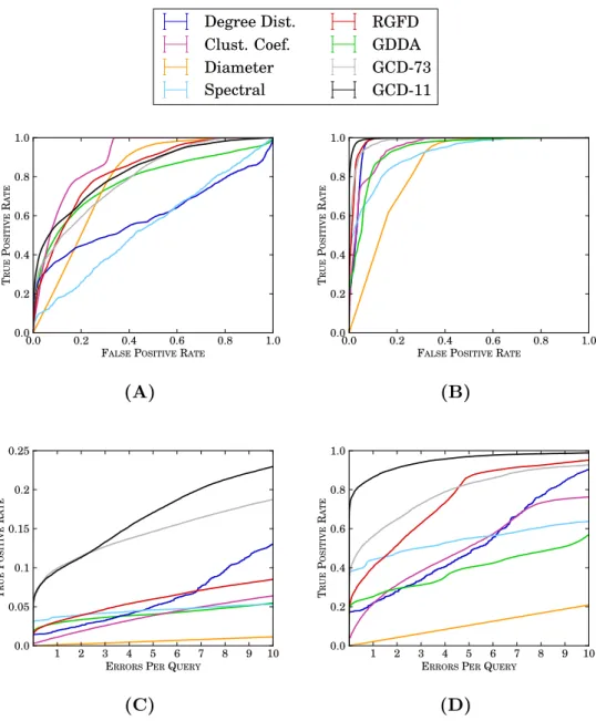
2.5 Computational Complexities of Network Distance Measures . 90

2.6 Author’s Contributions . . . 93

3 Analysis & Comparison of World Trade Networks 94 3.1 Motivation . . . 94

3.2 Topology of World Trade Networks . . . 97

3.3 E↵ect of Crude Oil Price Changes on the World Trade Network 99 3.4 Graphlet Change Profile of Global Recessions . . . 104

3.5 Graphlets and Economic Wealth Indicators . . . 107

3.6 E↵ects of a Country’s Network Position on its Crisis Patterns 109 3.7 Author’s Contributions . . . 112

4 Models of World Trade Networks 114 4.1 Motivation . . . 114

4.2 Model-fitting on Real-world Networks . . . 116

4.3 Models of World Trade Networks . . . 117

4.3.1 Gravitational Random Model . . . 121

4.3.2 Brokerage Model . . . 123

4.3.3 Analysing World Trade Network Organisation using the Brokerage Model . . . 126

4.4 Author’s Contributions . . . 129

5 Exponential-family Random Graph Modelling using Graph-let Terms 131 5.1 Motivation . . . 131

5.2 Graphlet Terms for Exponential-family Random Graph Mod-elling . . . 133

5.3 Implementation . . . 136

5.3.1 Algorithmic Details . . . 137

5.3.2 Validation of the Implementation . . . 142

5.4 Case Studies . . . 143

5.4.1 Lake Pomona Emergent Multi-Organizational Network 143 5.4.2 Protein Secondary Structure Network . . . 148

5.5 Model Degeneracy, Instability, and Sensitivity . . . 156

6 Conclusion 159

6.1 Summary of the Dissertation . . . 159 6.2 Future Directions . . . 164

6.2.1 Phylogeny Reconstruction from Metabolic Network Similarities . . . 164 6.2.2 Uncovering Topological Disease - Pathway Similarities 165 6.2.3 Improvements on the Graphlet Degree Vector

Simi-larities of Nodes . . . 168 6.2.4 Integration of Graphlet Correlation Distances with

ergm package . . . 170

List of Tables

1.1 Complexities of adjacency list and matrix representations . . 31 2.1 Dependencies for all 2- to 4-node graphlet orbits. . . 68 2.2 AUC, Maximum Accuracy, and AUCEP Q=10 scores of di↵

er-ent GCD versions . . . 80 2.3 AUC, Maximum Accuracy, and AUCEP Q=10 scores of di↵

er-ent network distance measures. . . 84 3.1 All significantly correlated changes in crude oil price and

trade network topology . . . 103 4.1 Summary of the sizes and densities of real-world networks . . 115 4.2 Pearson’s correlation coefficients of economic wealth

indica-tors and graphlet degrees of core-broker-periphery orbits . . . 127 4.3 Pearson’s correlation coefficients of economic wealth

indica-tors and graphlet degrees of orbit 58 for di↵erent year shifts . 130 5.1 The complete list of edge orbit - graphlet associations . . . . 139

List of Figures

1.1 Illustration of network representations . . . 32

1.2 Degree distribution and clustering spectrum of a network . . 34

1.3 Shortest path length, adjacency matrix, and Laplacian spec-tra of a network . . . 37

1.4 Graphlets and automorphism orbits . . . 39

1.5 Graphlet degree vector (GDV) computation . . . 40

1.6 Graphlet degree distributions of a network . . . 41

1.7 Networks generated from the seven random network models . 49 2.1 Illustration of redundancies among orbits 0, 2, and 3 . . . 63

2.2 Example graphlet that is used for explaining the redundancy weighting . . . 64

2.3 Non-redundant orbits of 2- to 4-node graphlets . . . 67

2.4 Graphlet orbit dependencies for orbit 21. . . 69

2.5 Graphlet correlation matrix computation . . . 71

2.6 Graphlet correlation matrices of four di↵erent networks . . . 72

2.7 3D embedding of model networks based on GCD-11 . . . 76

2.8 3D embedding of real-world networks based on GCD-11 . . . 77

2.9 Model clustering performances of di↵erent GCD versions . . . 81

2.10 Model clustering performances of di↵erent network distance measures . . . 83

2.11 Model clustering performance of di↵erent network distance measures on rewired networks . . . 87

2.12 Model clustering performance of di↵erent network distance measures on incomplete networks . . . 88

2.13 Model clustering performance of di↵erent network distance measures on sampled network properties . . . 91

3.2 The crude oil price and network topology changes that are significantly correlated based on Spearman’s Correlation Co-efficient . . . 101 3.3 The crude oil price and network topology changes that are

significantly correlated based on Phi Correlation Coefficient . 102 3.4 Graphlet change pattern during 1991 Global Downturn . . . 105 3.5 The graphlet count change patterns during crisis years . . . . 106 3.6 Canonical correlation analysis results on economic wealth

in-dicators and graphlet degrees of countries . . . 108 3.7 Brokerage score changes between 1962-2010 . . . 111 3.8 Peripheral score changes between 1962-2010 . . . 113 4.1 Model fit experiments on autonomous, Facebook, metabolic,

and protein structure networks . . . 118 4.2 Model fit experiments on autonomous, Facebook, metabolic,

and protein structure networks (cont.) . . . 119 4.3 Model fit experiments on world trade networks . . . 120 4.4 Comparison of gravitational random model with world trade

networks . . . 122 4.5 Comparison of brokerage model with world trade networks . . 124 4.6 Per year data-vs-model distances between brokerage and

grav-ity random models and world trade networks . . . 125 4.7 Economic wealth indicators vs. graphlet degrees of orbit 58 . 128 5.1 The edge automorphisms of all 2- to 5-node graphlets . . . . 137 5.2 A subgraph for illustrating the computation ofergm.graphlets

terms . . . 141 5.3 Lake Pomona emergent multi-organizational network . . . 145 5.4 The goodness-of-fit test results of the ERGM estimated for

the EMON data . . . 149 5.5 The protein structure network of matriptase-BPTI complexes 151 5.6 The goodness-of-fit test results of the ERGM estimated for

the network of matriptase-aprotinin complex . . . 155 5.7 Observed and model generated protein structure networks . . 156 6.1 The performance of metabolic network distances in

List of Abbreviations and Symbols

Network Representations

• G(V, E) = A network Gwith the node setV and edge set E. • |V|= The number of nodes in a network.

• |E|= The number of edges in a network. • A= Adjacency matrix of a network. • D= Diagonal Degree Matrix of a network. • L= Laplacian Matrix of a network.

Network Properties

• D(v) = Degree of node v.

• CC(v) = Clustering Coefficient of node v. • Cc(v) = Closeness Centrality of nodev.

• Cb(v) = Betweenness Centrality of node v.

• E(v) = Eccentricity of nodev.

• Ce(v) = Eccentricity Centrality of nodev.

• Ci(v) = Graphlet degree of node v for orbit i. Note that, i is an integer and i₂[0,72].

• CEi = The number of graphlets counted by placing edge orbit i on the flipped edge during the MCMC process of ERGM parameter esti-mation.

• GDV = Graphlet Degree Vector. • GCM = Graphlet Correlation Matrix.

Random Network Model Abbreviations

• ER = Erd¨os R`enyi Random Network Model. • ER DD= Generalized Random Network Model.

• SF BA = Scale-free Barabasi-Albert (Preferential Attachment) Model.

• SF GD = Scale-free Model with Gene Duplication and Divergence Events.

• GEO = Geometric Random Network Model.

• GEO GD= Geometric Random Network Model with Gene Dupli-cation and Divergence Events.

• ST ICKY = Stickiness-index based Random Network Model. • GR= Gravitational Random Network Model.

• ERGM = Exponential-family Random Graph Model.

Network Distance Measures

• GCD = Graphlet Correlation Distance.

• GCD 11 = Graphlet Correlation Distance that is computed from the 11 non-redundant orbits of 2- to 4-node graphlets.

• GCD 73 = Graphlet Correlation Distance that is computed from the 73 orbits of all 2- to 5-node graphlets.

• RGF D=RGF Distance= Relative Graphlet Frequency Distance. • GDDA = GDD Agreement= Graphlet Degree Distribution

Economic Wealth Indicators

• RGDP L= Gross Domestic Product - derivation method 1 • RGDP L2 = Gross Domestic Product - derivation method 2 • RGDP CH = Gross Domestic Product - derivation method 3 • KC = Consumption Share

• KG= Government Consumption Share • KI = Investment Share

• OP EN K = Openness • P OP = Population

• LE = Level of Employment • BCA= Current Account Balance

Other Abbreviations

• M CM C = Markov-Chain Monte-Carlo.

• M P LE = Maximum Pseudo-Likelihood Estimation. • M LE = Maximum Likelihood Estimation.

1 Introduction

1.1 Motivation

A network (graph) is a mathematical representation of relational data in which nodes (vertices) correspond to the entities in a system, and edges (arcs) correspond to relations among those entities [145]. Networks are widely used for representing complex systems from many di↵erent domains, such as economics [10, 17, 26, 30, 52, 93, 170, 186], biology [46, 53, 65, 96, 167, 171, 197], sociology [28, 119, 123, 124, 193] and technology [116, 206]. Network based analysis of these systems sheds light on their organization, the mechanisms that govern their formation and evolution, and the rela-tions among their elements. However, exact solurela-tions of the network anal-ysis problems that produce these insights are intractable as the number of possible network configurations increases exponentially with the size of the networks. In this dissertation, we propose solutions for two of these network analysis problems: (1)Network Comparison, and (2)Network Modelling.

Many real-world complex systems are dynamic which means that these systems have di↵erent configurations at di↵erent time points; e.g., world trade networks [34], gene expression networks [61, 103], autonomous net-works [206]. The time points at which these systems change and possible causes of these changes can be identified by systematically comparing the topologies of networks that correspond to di↵erent snapshots of the system. It is also possible to transfer knowledge among di↵erent real-world domains by identifying the topological similarities among corresponding networks.

Identifying the complete list of topological di↵erences between two net-works requires solving the subgraph isomorphism problem [35]. Given two graphsGand Has input, the subgraph isomorphism problem asks whether G has a subgraph that is isomorphic to (i.e., has exactly the same topol-ogy as) H. This problem is shown to be NP-Complete [63], meaning that there are no polynomial-time exact solutions, but only approximate

so-lutions (i.e., heuristics) for this problem. The network comparison prob-lem is NP-Complete due to the underlying subgraph isomorphism probprob-lem. The most sophisticated methods for the network comparison problem are based on graph spectra [190, 201] and small subnetworks including network motifs [140] and graphlets [156, 157]. Among these network properties, graphlets are defined as small, connected, non-isomorphic, and induced subgraphs of a network. We investigate the redundancy and dependency relations among di↵erent graphlet properties, and improve the available techniques further by proposing a new network topology descriptor based on this investigation. We use this new topology descriptor to quantify the topological similarities between two networks.

We apply our new methodology to the world trade network. The recent global recession and the unstable nature of the world economy is encouraging researchers to gain a deeper understanding of the functional mechanisms of the world economy. World trade is one of the factors that shape the world economy. Understanding the organizational principles of the world trade network sheds light on the dynamics of the world economy, and guides the economists to minimize the systematic breakdown risks of the world economy. With this aim, we investigate the topological organization of the world trade networks, the link between the changes in world trade network topology and the global recessions, and the e↵ects of a country’s position on its wealth.

Given a networkG(V, E) that contains|V|nodes, there are 2(|V2|) possible

network configurations that G can be in when the network is undirected; i.e., when each pair of nodes in the network may or may not be connected by an edge without any specific edge orientation. A network model is a set of rules that describes the formation and evolution of networks by picking a subset of the possible configurations [145]. The model-fitting problem asks whether an input network is in the subset of configurations that is picked by the evaluated network model or not. Network comparison methods can easily answer this question by quantifying the topological similarities among the input network and the network configurations defined by the model [76, 156, 163].

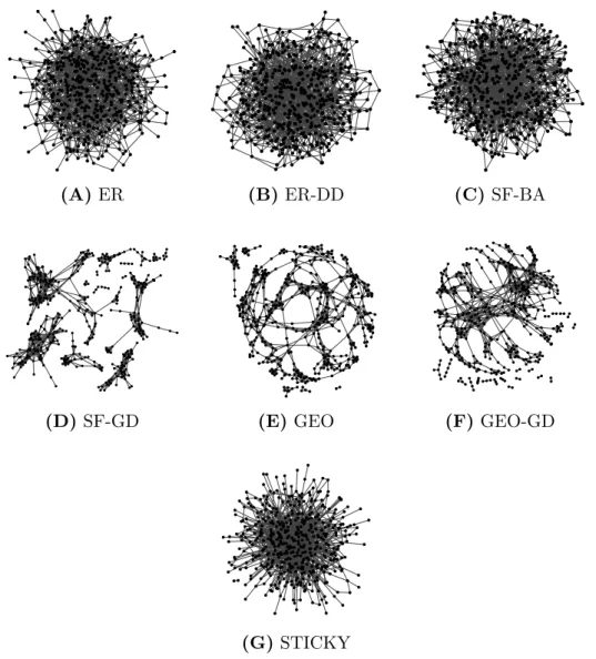
We use our new network distance measure to identify the models of five di↵erent network types: (1) Autonomous Networks [206], (2) Facebook Net-works [193], (3) Metabolic NetNet-works [98], (4) Protein Structure NetNet-works

[143], and (5) World Trade Networks [34]. Furthermore, we propose two new random network models that describe the topology of the world trade networks better than existing models. One of these models is defined solely based on the graphlet properties of the network, and fits world trade net-works better than the other models. The superior performance of this model encourages us to extend the applicability of graphlet properties from net-work comparison problems to netnet-work modelling, and to implement a new framework that enables network modelling based on any combination of graphlet properties. Moreover, this new network modelling framework en-ables defining models that uncover the links among the node attributes and their position in the network.

In the rest of this section, we first explain the di↵erent types of real-world networks that are analysed in the scope of this dissertation. Then, we introduce the relevant graph-theoretic concepts on network comparison and modelling. We provide a brief literature survey on the network comparison problem and the state-of-the-art heuristics on it. Following this, we describe well-known random network models, and the methodologies for evaluating their fit on an input network. As our main focus in this dissertation is the analysis of world trade networks, we provide a brief literature survey on the main properties and well-known models of world trade networks. We conclude this section with the dissertation outline.

1.2 Real-World Networks

Relational data from many di↵erent real-world domains are modelled and analysed as networks; e.g., financial and world trade networks from the eco-nomics domain, protein-protein interaction, genetic interaction, metabolic interaction, protein structure, and signalling networks from biological do-main, friendship and collaboration networks from social dodo-main, and au-tonomous networks from technological domain. These networks appear in many di↵erent forms, and represent di↵erent types of information about these systems. Mining the networks from these domains uncovers valuable insights into understanding the functional mechanisms embedded in them.

Networks can appear as directed or undirected; based on the existence of an ordering among the node pairs that form the edges. Similarly, the edges can be unweighted or weighted for representing their relative

impor-tance in the network. In this dissertation, we mainly focus on undirected and unweighted networks, since the networks of this form still carry valu-able amount of information, while the methods for analysing the structural properties of these networks are much more advanced and scalable to large networks. For this reason, we process the datasets that appear as directed or weighted to obtain unweighted and undirected network representations.

In this section, we introduce di↵erent forms of networks from the four above listed real-world domains and explain how we collect and process the network datasets that are analysed in this study.

1.2.1 Economic Networks

Networks are widely used for representing and analysing di↵erent types of complex micro-scale and macro-scale economic information; e.g., interbank relation networks where banks are the nodes and the edges represent the credit-debt relations among them [17, 93], investment (inter-company) net-works where nodes represent companies and edges link the companies that co-invest on the same portfolio [10, 26], supply-chain networks where nodes correspond to organisations (e.g., companies) and edges represent the flow and movement of materials and information [30, 186], and world trade net-works where nodes correspond to countries and edges correspond to the trade links among them [52, 170]. Among this variety of economic network types, we focus on the world trade networks because of their importance in representing the global money flow, and the macro scale information that can be mined through the topology of these networks. World trade networks naturally appear as directed and weighted networks, where the edge direc-tions represent the import/export reladirec-tions, and the edge weights represent the volume of trade. However, depending on the applied network analysis techniques, unweighted and undirected versions of these networks have also been used.

TheUnited Nations Commodity Trade Statistics(UN Comtrade) database is the most reliable and complete source for the world trade data. UN Com-trade contains the world Com-trade relations data since 1962 [34]. The records of the database are formed by the individual declarations of the countries. This method of dataset construction sometimes cause inconsistencies in the database; e.g., country A declares that it imported products of X$ worth

from countryB, whileB declares that it exported products of Y$ worth to countryA. These inconsistencies need to be resolved while constructing the world trade networks from UN Comtrade [170].

The world trade data in UN Comtrade is grouped into categories with re-spect to their commodities, which enables constructing commodity-specific networks; e.g., trade network of Food and Live Animals, Mineral Fuels, Chemicals, Machinery and Transport Equipment. The trade data is orga-nized with respect to 10 di↵erent commodity categorization standards; i.e., STIC (4 di↵erent versions), HS (5 di↵erent versions), and BEC standards.

Construction of Analysed Economic Networks. From the economic domain, we analyse only the world trade networks in the scope of this study. We obtain the world trade data from the UN Comtrade database [34], and construct commodity specific networks from this dataset using the Standard International Trade Classification (SITC) Revision 1 standard. The prod-ucts that are traded in 1960s can be very di↵erent from what is being traded now; e.g., with the recent developments in the technological era, new prod-ucts such as laptops, tablet computers, mobile phones appeared after 1990s. SITC Rev. 1 is preferred over the other commodity classification standards since it best covers the range trade products from 1960s to now. SITC Rev. 1 groups the trade products into 10 commodities. For each of these com-modities and also for the total trade, we generate 49 trade networks, one for each year between 1962 and 2010 (producing a total of 11_⇥49 = 539 networks; one network per each commodity - year combination).

In order to resolve the issues caused by the inconsistent import/export declarations to UN Comtrade, we assign confidence scores to each country’s import/export declaration. The declaration confidence score of a country, X, is defined as the absolute di↵erence between the sum of all imports/ex-ports that are declared byX and the sum of all imports/exports that are declared by the trade partners ofX. The countries with smaller declaration confidence scores are accepted to be more reliable. We determine the weight of a directed edge from countryAto countryB by taking the trade amount declared by the more reliable country.

The fact that most countries have both import and export trade makes the trade network inherently directional. However, since we are only interested in the presence or absence of an interaction between countries, we generated undirected networks and weighted the edges by summing import and export

trade volumes; e.g., given that countryAexports X$ worth of products to country B and country B exports Y$ worth of products to A, the trade volume (i.e., the weight of the undirected edge) betweenA and B is equal to (X +Y). For making the networks unweighted, we filter the lowest weighted edges until 90% of the total trade in the network remains. This filtering produces undirected and unweighted networks that represent the most important trade relations in the network, while covering at least 90% of the money flow in the world. This filtering is necessary for observing the graphlet properties of the world trade network better, since currently graphlets do not support analyses of weighted and directed networks. 1.2.2 Biological Networks

Di↵erent types of relational data in biology are analysed using networks. The main types of biological networks are protein - protein interaction net-works, metabolic netnet-works, protein structure netnet-works, disease netnet-works, genetic interaction networks, transcriptional regulatory networks, and sig-nal transduction networks. These networks are described as follows:

Protein-Protein Interaction Networks: Proteins are the main build-ing blocks of almost all processes in an organism. They almost never func-tion alone but bind to each other. Protein-Protein Interacfunc-tion (PPI) net-works represent the binding information among all proteins of an organism; nodes representing the proteins and edges representing physical interac-tions (bindings) between two proteins. Protein interaction networks appear as undirected graphs. Although the edges of these networks are normally unweighted, some studies assign weights representing the confidence on the existence of the interaction [188].

The two main experimental techniques that most protein interaction in-formation is obtained from are Yeast-2-Hybrid (Y2H) screening [94, 95, 165, 172, 183, 195] and Protein Complex Purification methods using Mass-Spectrometry (MS) experiments [33, 64, 108, 162]. Y2H screening experi-ments identify pairwise protein interactions. However, the interactions iden-tified by this technique contain many false positives since the experiments are performed in yeast nucleus regardless of the organism the genes are taken from. The genes from di↵erent organisms may not behave as in their native

environment when they are in yeast nucleus. It is estimated that 50% of the interactions identified by a Y2H experiment are noisy [197], although the Y2H experiment systems have recently improved to produce more accurate results. MS Experiments do not identify binary protein interactions as Y2H experiments do, but they identify protein complexes. In this technique, bait proteins are tagged and used as hooks. The proteins that interact with the bait (i.e., the preys) are separated from the culture together with the bait protein, indicating the existence of a protein complex. The main problem with MS experiments is the extraction of binary interactions from identified complexes. The two models that are commonly used for this purpose are the spoke model and the matrix model. The spoke model assumes that the bait protein interacts with all prey proteins, and none of the prey proteins interact with each other. The matrix model assumes that all protein pairs in the identified complex interact with each other. It is obvious that these two models are abstractions over the underlying structure of the protein complex. The matrix model introduces many false positives while the spoke model introduces many false negatives together with some false positives.

Another problem with protein interaction networks is their incomplete-ness. For a network with n nodes, there exists n(n 1)/2 possible inter-actions. There are approximately 6,000 proteins in yeast, raising the need for testing ⇠18 million interactions for their existence. In addition to this huge number of possibilities, most of the protein interaction identification studies are focussed on a certain process or disease, leaving the other parts of the protein interaction network uncovered. Saccharomyces Cerevisiae is the most well-studied organism for protein interaction networks. The total number of protein interactions inSaccharomyces Cerevisiae is estimated to be between 150,000 - 370,000 [75]. However, the number of protein inter-actions identified forSaccharomyces Cerevisiae as of August 2013 is 81,839 [181] (statistics of BioGRID database - version 3.2.103), showing that even the interactome for this well-studied organism is only_⇠50% complete.

The main public databases that contain protein interaction networks are Saccharomyces Genome Database (SGD) [29], Munich Information Center for Protein Sequences (MIPS) [134], the Database of Interacting Proteins (DIP) [203], the Online Predicted Human Interaction Database (OPHID) [19], Human Protein Reference Database (HPRD) [152, 155], the General Repository for Interaction Datasets (BioGRID) [181, 182], and the Search

Tool for the Retrieval of Interacting Genes / Proteins Database (STRING) [188]. Some of these databases contain interactions that are predicted with computational techniques but not validated experimentally; e.g., OPHID, STRING. These predicted interactions should be used with caution or ex-cluded in most analyses, since protein interaction networks already contain high levels of experimental noise which will exponentially increase with the inclusion of predicted interactions.

Although we also applied our methodology on the PPI networks that are collected from BioGRID, we keep the results of these experiments out of the scope of this dissertation, since our results were similar to the results of previous studies on these networks.

Metabolic networks: Biochemical reactions are crucial for keeping a cell in homoeostasis state (the stable state that a normal cell should be in). Metabolic networks explain the collection of all biochemical reactions that occur in a cell [96, 189]. A metabolic network is a bipartite network of metabolites and reactions, where each metabolite is connected with the reactions that it is involved in. Metabolites can be small molecules such as glucose, amino acids or larger molecules such as polysaccharides, glycan. The biochemical reactions are represented by directional edges since they represent chemical conversion of the metabolites from one form to another. However, most biochemical reactions are bidirectional; i.e., the e↵ects of most reactions can be reversed. For this reason, it is also safe to represent metabolic networks as undirected networks.

The main data source for the metabolic networks is the KEGG database [98]. GeneDB [79], BioCyc [99], EcoCyc [103], MetaCyc [107], and ERGO [149] databases also contain biochemical reaction information for di↵erent species.

The metabolic network of all species can be viewed as a very large sin-gle network that contains all possible reactions in all species. Enzymes, which are proteins that catalyse the biochemical reactions and synthesized from the genome, cause the di↵erence among the metabolic networks of dif-ferent species. If the gene that produces the enzyme does not exist in a species, the corresponding biochemical reaction does not occur within the cell of the species. For this reason, it is common practice that reactions are replaced by the enzymes that catalyse them, or even by the genes and

proteins that produce that enzyme in metabolic networks. This replace-ment generates di↵erent metabolic network representations; e.g., networks in the form of metabolite – enzyme, metabolite – protein, and metabolite – gene interactions. The bipartite metabolic networks can be represented as simple graphs, by removing the reaction nodes or metabolite nodes, and connecting the remaining nodes if they are at distance 2 to each other in the bipartite network. This simplification produces metabolic networks in the form of metabolite – metabolite, reaction – reaction, enzyme – enzyme, protein – protein, and gene – gene networks. The particular choice on the network representation to be used depends on the focus of the study and the capabilities of the network analysis tools.

Construction of Analysed Metabolic Networks. We analyse the metabolic networks in the form of enzyme – enzyme interactions. We obtain the metabolic network information of 2,301 species from KEGG database [98] (downloaded in February 2013), and construct a metabolic network for each species by linking a pair of enzymes if they catalyse reactions that share a common metabolite. We excluded networks containing less than 100 nodes from our analysis.

Protein Structure Networks: The tertiary (3D) structure of a protein provides insights into both characterization of the protein [53, 86, 125, 185, 202] and also identification of its binding domains [68, 135]. The infor-mation provided by the tertiary structure of the protein complements the information provided by its sequence. Protein structure networks represent the tertiary structures of proteins. The nodes in these networks correspond to the amino acids in a protein. Two amino acids are connected if they are in contact; i.e., the distance between their alpha-carbons is less than a dis-tance threshold; a common threshold being 7.5 ˚A (Angstrom, that is 10 10

meters). The Structural Classification Of Proteins (SCOP) database is the main information source for the tertiary structure information of proteins [143]. This database contains coordinates that represent the relative posi-tions of the alpha-carbons of each amino acid in a protein. Furthermore, it provides information about the classification of the protein in terms of class, fold, family and superfamily. RCSB Protein Data Bank (PDB) provides an interface for searching the structural information about specific proteins in SCOP [14].

Construction of Analysed Protein Structure Networks. We use the standard distance threshold of 7.5 ˚A while constructing these networks, and construct the networks of all protein structures in the Astral 40 com-pendium v1.75B [143] (Downloaded in January 2011). When we filter out the protein structures with more than 40% of sequence identity or less than 100 amino-acids, we obtain the protein structure networks of 8,226 proteins.

Disease Networks: So far, diseases have been grouped and studied in terms of the similarities of their symptoms and the organs they a↵ect. This trend is shifting towards relating diseases based on their genetic origins, rather than their phenotypical similarities. In this respect, Goh et al. [65] defined the first disease – disease association network. In this network, nodes correspond to diseases and two nodes are connected when the two corresponding diseases are linked with at least one gene in common. They further extend the disease – disease network into a bipartite disease – gene network, where the genes and diseases are connected if there is a causal relationship between them. Hidalgo et al. [81] define disease – disease networks in a di↵erent manner, by evaluating the common occurence of the diseases in the same person at the same time, which is called commorbidity of diseases. Furthermore, Hu et al. [89] produced a disease – drug network by analysing the genomic expression profiles of human diseases and drugs.

Most disease networks are based on the known disease – gene associa-tions. There are many databases that contain disease – gene associations; e.g., Online Mendelian Inheritance in Man (OMIM) [70], Functional Dis-ease Ontology Annotations (FunDO) [148], Comparative Toxicogenomics Database (CTD) [42], Genetic Association Database (GAD) [12]. The Dis-GeNet database [11] integrates the disease – gene associations from many of these individual databases, and provides a single dataset containing all experimentally validated and predicted disease – gene associations.

Analyses of disease networks is out of the scope of this dissertation, but we have some ideas on constructing disease – disease association networks as a future direction (explained in Section 6.2.2).

Genetic Interaction Networks: Genetic interactions are defined based on the e↵ect of combined gene deletions on a given phenotype. The mul-tiplicative phenotype fitness model assumes that the combined deletion

of two independent genes is expected to show a phenotype which is the multiplication of the phenotype e↵ects observed after single gene deletions [36, 46, 102, 147, 191, 192]. The most commonly used phenotype for mea-suring the e↵ects of gene deletions is the colony size; i.e., the number of cells in the culture. If the deletion of two genes results with a phenotype worse than the expected phenotype, then these two genes are accepted to have negative genetic interactions. Synthetic lethality, synthetic sickness, synthetic growth defect interactions are examples of negative genetic in-teractions. Deletion of two genes may also result with a better phenotype than expected, showing apositive genetic interaction. Genetic interactions are identified by the synthetic genetic array (SGA) [191] or synthetic lethal analysis by microarray (SLAM) [147] experiments. Dixon et al. [46] pro-vides a detailed survey of di↵erent genetic interaction types, experimental systems for extracting genetic interaction information, and possible scenar-ios for the occurrence of the genetic interactions. In genetic interaction networks, nodes represent the genes and edges connect two genes if the ob-served phenotype after the deletion of genes is unexpected. These network are undirected. Edges can be weighted based on the Z-scores of the observed phenotypes.

The public databases for obtaining genetic interaction data are BioGRID [181] and Flybase [194]. Saccharomyces Cerevisiae, Schizosaccharomyces Pombe,Drosophila Melanogaster and Caenorhabditis Elegans are the only well-studied organisms for genetic interactions in the last 10 years. However, a recent study by Lin et al. [121] revealed a genetic interaction network forHomo Sapiens indicating the forthcoming genetic interaction data from other species.

Genetic interaction networks are not analysed in the scope of this disser-tation due to their limited availability.

Transcriptional Regulatory Networks: Transcription regulatory net-works describe the relations between genes in terms of their e↵ects on each other’s transcription [171]. The nodes of these networks are genes. A di-rected edge is drawn from node A to node B if the product of gene A (protein A) regulates the transcription of gene B. Protein A binds to the regulatory DNA regions of geneB which may result with over-expression or under-expression of geneB. These interactions are identified by measuring

and comparing the relative mRNA levels of the genes. The well-studied organisms for their transcription regulation mechanisms areSaccharomyces Cerevisiae and Caenorhabditis Elegans. The databases that contain tran-scription regulation information are EcoCyc [103], KEGG [98], RegulonDB [61], Reactome [38], TransPath [167] and TransFac [131].

Analysis of transcription regulatory networks is out of the scope of this dissertation.

Signal Transduction Networks: These networks explain the complex signalling mechanisms inside a cell [167]. The nodes of these networks are proteins and the directed edges connecting these proteins represent the sig-nals propagated from one protein to another. These networks are used for modelling the cellular responses to di↵erent internal and external stimuli by means of pathways. These networks are especially important for the analysis of diseases, since most diseases are caused by errors occurring in the transduction of the signals in these networks. However, the availabil-ity of these relations is limited. Therefore, analysis of signal transduction networks is out of the scope of this dissertation.

1.2.3 Social Networks

Networks have been used for representing a wide-range of complex social sys-tems; e.g., friendship networks [132, 193], collaboration networks [47, 119], citation networks [28, 118], e-mail networks [119], co-authorship networks [119, 123], co-purchasing networks [117, 124]. Among these network types, friendship networks, in which nodes represent people and edges connect people with friendship relations, are of particular interest due to the re-cent boom in online social networking applications; e.g., Facebook, Twitter, Instagram, Google+. The recent developments in online social networking raised a new set of interesting network analysis questions; e.g., What are the main characteristics of social networks?, How do friendship networks form?, What are the principles governing the evolution of these networks?, How can the social media be used most e↵ectively for viral advertising purposes? Though online social networking applications are important data sources for obtaining friendship networks, collecting these networks is an extremely challenging task. These networks contain millions of nodes and edges, and

the topology of these networks change dynamically by added and deleted users/connections at every second. It is very hard to take a snapshot of these networks at a particular time point. For this reason, these networks are mostly obtained by network crawlers [112], which are small software programs that sample di↵erent chunks of the network data in parallel in order to capture the network structure in a fast and accurate way. Network crawling based construction of friendship networks comes with the cost of high levels of noise and incompleteness in the obtained networks. Because of the difficulty of obtaining social networks, there are not many publicly available large-scale datasets.

Construction of Analysed Social Networks: We analyse the friend-ship networks that are collected Traud et al. [193]. These friendfriend-ship net-works are obtained from the Facebook friendship links of the members of

⇠ 100 American universities. The nodes of these networks correspond to Facebook user accounts that are linked to an American University as a stu-dent or sta↵, and the links correspond to the Facebook friendship relations among the users. These networks are complete subnetworks of the whole Facebook network in September 2005.

Stanford Large Network Dataset Collection [116] contains some addi-tional social networks of Facebook, Google+, and Twitter. However, these datasets are collected on a voluntary basis by some smartphone applications that the users need to install. For this reason, they are highly incomplete. 1.2.4 Technological Networks

The World Wide Web was developed in 1990 and has been one of the most significant inventions of all times since then. It is indeed one of the best ex-amples of networks; nodes corresponding to electronics such as computers, laptops, mobile phones, satellites with di↵erent IP addresses, and edges cor-responding to direct physical communication channels among them. Con-sisting of millions of dynamically changing nodes and edges, it is challenging to obtain a snapshot of this huge system. Autonomous systems provide an abstract representation of the World Wide Web; an autonomous system being a subset of routers in the World Wide Web. In autonomous sys-tem networks, nodes correspond to autonomous syssys-tems. The autonomous systems that exchange information are connected by edges, forming a

“who-talks-to-whom” network.

Construction of Analysed Technological Networks. The Univer-sity of Oregon Route Views Project [206] produced one of the best datasets of autonomous networks. Analysing the Border Gate Protocol logs of au-tonomous systems in Oregon University on a daily basis, 733 networks repre-senting the traffic flow on a single day are constructed [116]. We downloaded these 733 autonomous networks from SNAP database on 09/08/2012. Each of these networks represents daily communication data between autonomous systems of Oregon University for the time period between 8th November 1997 and 26th _{May 2001.}

1.3 Concepts on Networks

A graph (also called network) is a mathematical representation of a set of objects and the relations among them. A graph is denoted byG = (V, E) where V is the set of nodes that represent the objects, and E is the set of edges that define the relations among the elements of V. A graph is undirected if the edges of the graph have no orientation; i.e., ₈(u, v) ₂E : (u, v) = (v, u). A graph isdirected when the edges of the graph are defined as a set of ordered tuples; i.e., ₈(u, v) ₂ E : (u, v) ₆= (v, u). A graph is weighted if a real-valued property is assigned to the edges of the graph. A simple graph is an undirected and unweighted graph which contains no self-loops (₈v₂V : (v, v)₂/ E) or multiple edges. Theneighbourhood of nodev, N(v), is the set of nodes that are adjacent tov. Apath between nodesuand vis an ordered set of edges that need to be traced for reaching from nodeu to nodev without visiting any node more than once. Acycle is a path that starts and ends at the same node. A graph isconnected if there exists a path from every node to every other node, otherwise it is disconnected. A graph H(V0, E0) is a subgraph of G(V, E) if V0 _✓ V and E0 _✓ E. A subgraph H(V0, E0) ofGisinduced if it contains all the edges inGbetween the nodes inV0; otherwise it is apartial subgraph. An undirected, connected graph is atree when any two vertices are connected by exactly one simple path; i.e., there are no loops in the graph. Eliminating any edge from a tree makes the graph disconnected, and connecting any two disconnected nodes of a tree forms a cycle. A singly connected network (also known as apolytree) is a directed acyclic graph with the property that ignoring the directions on the

edges yields a tree.

Networks can be represented in computer memory using di↵erent data structures. The particular choice of a data structure depends on the com-putational requirements of the software in which the networks are used. The complex information encoded in these data structures do not provide a direct understanding of the network structure. Network properties sum-marize the main topological characteristics of the network and provide an easy-to-understand description of the network structure. Identifying the exact topological correspondence between two networks is computationally intractable, due to the underlying subgraph isomorphism problem that is NP-Complete [35]. For this reason, there are only approximate solutions (i.e. heuristics) to the network comparison problem. These heuristics use the network properties (statistics) that summarize the network topology. In the rest of this section, we first introduce di↵erent data structures for rep-resenting networks in computer memory, and discuss their advantages and disadvantages. Then, we describe the topological network properties that summarize the information encoded in these representations. We conclude this section by describing the network comparison heuristics that are based on the network properties.

1.3.1 Network Representations

There are two fundamental data structures for representing a graphG(V, E) with _|V_| nodes and _|E_| edges [115]: (1) adjacency list, and (2) adjacency matrix. Theadjacency list ofG(V, E) is a_|V_|dimensional arrayAL, where each element of the arrayAL[n] corresponds to a nodenin the network and is linked to the list of nodes that are adjacent ton. For representing weighted networks, an extra list of edge weights should be kept for each node. The adjacency matrix of G(V, E) is a |V|⇥|V| matrix A, where A[u, v] is a non-zero value when nodesuandv are connected, and equal to 0 otherwise. A is a symmetric matrix when Gis undirected. For representing weighted networks, the edge weights can be encoded in the value ofA[u, v].

Both representations have their own advantages. Table 1.1 summarizes the worst-case space complexities of representing a network in computer memory with these data structures, together with the worst-case time com-plexities of common network operations when performed on these

repre-sentations; i.e., adding a node into the network, adding an edge into the network, deleting a node from the network, deleting an edge from the net-work, and searching for the existence of an edge in a network. Note that, in practice, these complexities are lower, especially when working with sparse graphs. For sparse graphs, the adjacency list representation is more mem-ory efficient than adjacency matrices. Moreover, the computational cost of adding or deleting a node from the network is high for the adjacency matri-ces, since the size of the matrix changes and the whole matrix needs to be allocated again. On the contrary, edge operations are faster on adjacency matrices, as the existence and the weight of an edge can be directly changed from the relevant matrix element.

Adjacency List Adjacency Matrix Storage O(|V|+|E|) O(|V|2₎

Add Node O(1) O(_|V_|2₎

Add Edge O(1) O(1)

Delete Node O(|E|) O(|V|2₎

Delete Edge O(_|E_|) O(1)

Search Edge O(_|V_|) O(1)

Table 1.1: Comparison of adjacency list and adjacency matrix representa-tions with respect to the space complexities and time complexities of performing simple graph operations. These complexities are based on the assumption that node indexes are known.

The space allocated for the adjacency matrix can be used more e↵ectively by combining di↵erent types of information about the network in this rep-resentation. For example, the diagonal elements of the adjacency matrix of a simple graph are all equal to 0 since the graph does not contain self-loops. Therefore, the space allocated for the diagonal elements can be efficiently used for representing other node-specific information. TheLaplacian matrix of a graphLdoes this by encoding the degrees (i.e., the number of links that the nodes have) into the diagonal elements of the adjacency matrix. LetD be the diagonal degree matrix of a network; which is a|V|⇥|V|matrix with diagonal elements, D[u, u], being equal to the node degrees and all other elements being equal to 0. The standard combinatorial Laplacian matrix,

Network -

G

Adjacency List -

AL

Adjacency Matrix - A

Laplacian Matrix -

L

Figure 1.1: The adjacency listAL, adjacency matrix A, and Laplacian ma-trix L representations of a small network, Gex. Panel A illus-trates the small network, Gex. Panel B, C, and D respectively correspond to the adjacency list, adjacency matrix, and Lapla-cian matrix representations of the networkGex.

L, of a network is computed from the adjacency matrix A and diagonal degree matrixDas:

L=D A. (1.1)

The adjacency list (AL), adjacency matrix (M), and Laplacian matrix (L) representations of a small example network,Gex, is illustrated in Figure 1.1. 1.3.2 Network Properties

The properties that summarize the topological characteristics of a network fall into two categories: (1)Global Network Properties, that give an overall view of the network with respect to all nodes and edges (i.e., degree distribu-tion, clustering coefficient, shortest path lengths, centrality measures, and graph spectrum), and (2)Local Network Properties, that evaluate the

topol-ogy of a network in terms of its subgraphs (i.e., network motifs, graphlets). Global network properties are useful statistics that provide a simplified de-scription of the network topology. However, these properties sometimes fail to di↵erentiate between networks with completely di↵erent topologies. Independent of the amount of information that is embedded in the global network properties, these properties are very sensitive to noise in the net-work data, as they evaluate the topology of a netnet-work as a whole. The local changes in the network (e.g., deletion of a node, removal of an edge) might cause these properties change tremendously, although the structure of the network is still preserved for the rest of the network. Local network properties, which describe the network in terms of its subgraphs, would not su↵er from these problems as most of the subgraphs in the network would not be a↵ected from these local changes.

In the rest of this section, we describe the global and local network prop-erties in detail, and illustrate them on the example network, Gex, that is shown in Figure 1.1–A.

Global Network Properties

The simplest global network property is the node degree. The degree of a node is the number of links that the node has to other nodes in the network. For example, in Gex, the degree of node A is 1 and the degree of node B is 3. Average degree of a network is the arithmetic average of the degrees of all nodes in the network. The average degree ofGex is equal to (1 + 3 + 2 + 3 + 3 + 2)/6 = 2.333. If the network is directed, then two di↵erent degree definitions apply: (1)In-degree of a node is the number of links which point to the node, and (2) Out-degree of a node is the number of links which originate from the node. The degree distribution of a node is the distribution ofP(k), where P(k) is the probability that a randomly selected node has degreek. Figure 1.2–A illustrates the degree distribution ofGex. The highest degree nodes of a network are calledhubs.

The clustering coefficient of a node v, Cv, is the probability that two neighbours of a node are linked by an edge. When defined, it is computed as: Cv= T(v) deg(v) 2 = 2⇥T(v) deg(v)⇥(deg(v) 1), (1.2) where deg(v) is the degree of node v and T(v) is the number of triangles

through node v. Clustering coefficient is a measure of the degree to which nodes in a graph form transitive relations. For example, inGex, the cluster-ing coefficient of node B is 0 since its neighbours are not connected, while the clustering coefficient of node D is equal to 0.333 as there is one link between the three neighbours of D. Average clustering coefficient is the arithmetic average of the clustering coefficients of all nodes in the network. It represents how densely connected the network is. The average clustering coefficient of Gex is equal to 0.278. The clustering spectrum, C(k), is the distribution of average clustering coefficients of all degree k nodes, over all k. Figure 1.2–B illustrates the clustering spectrum ofGex.

(A) (B)

Figure 1.2: Global network properties of the network, Gex (Figure 1.1–A). The illustrated network properties are: Panel A – degree distri-bution, Panel B – clustering spectrum.

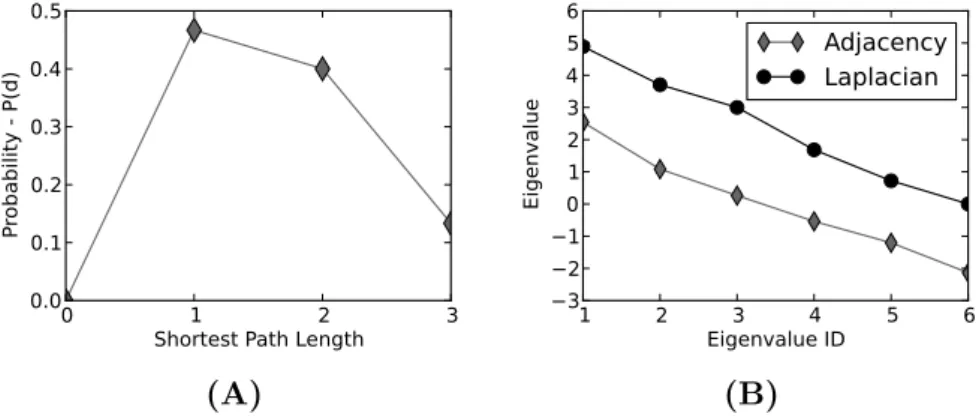
A shortest path between two nodes is a path that contains the minimum number of edges. Thedistance between two nodes is the length of a short-est path between two nodes; i.e., the number of edges in a shortshort-est path. For example, inGex, there are two shortest paths between nodesA and E: (1) the path A-B-D-E, and (2) the path A-B-C-E. The lengths of these shortest paths are 3 since these paths contain 3 edges. The distances be-tween the nodes are used for describing how spread the network is. The diameter of a network has two definitions: (1) the maximum shortest path distance among all pairs of nodes (e.g., the diameter is 3 forGex), and (2) the average of shortest path distances of all node pairs (e.g., the diameter is 1.667 forGex). In this dissertation, we use the first definition of diameter unless otherwise is explicitly stated. Thespectrum of shortest path lengths

is the distribution of probabilitiesP(d), whereP(d) is the probability that the distance between two randomly selected nodes are separated from each other with distance d, over all d. Figure 1.3–A illustrate the spectrum of shortest path lengths forGex.

Centrality of a node measures the relative topological importance of a node within a graph. There are five well-known centrality measures: (1) degree centrality, (2) closeness centrality, (3) betweenness centrality, (4) ec-centricity centrality, and (5) K-shell decomposition. The simplest centrality definition is thedegree centrality that is defined as the number of links in-cident upon a node. The degree centrality assumes that the importance of a node increases together with the number of its neighbours. Closeness centrality,Cc(v), is another centrality measure that evaluates the distances from a node to all other nodes. It is computed as:

Cc(v) =

1

P

u2V dist(u, v)

, (1.3)

where dist(u, v) is the distance between nodes u and v. For example, in Gex, the closeness centralities of nodes Aand D are respectively 0.091 and 0.143; higher values representing more central nodes. Betweenness central-ity,Cb(v), is a more detailed centrality measure that evaluates the number of shortest paths in the network that pass through the node. The betweenness centrality is computed as:

Cb(v) = X s6=t,s6=v,v6=t st(v) st , (1.4)

where st is the total number of shortest paths between nodes s andt and st(v) is the number of shortest paths between nodes s and t that pass through v. In Gex, the betweenness centrality of node A is 0 since none of the shortest paths in the network pass through A. On the contrary, the betweenness of nodeD is 0.3 highlighting its central role in connecting nodes. The eccentricity of a node is the maximum of the shortest path distances between the node and all other nodes in the network. Eccentricity centrality,Ce(v), is computed as:

Ce(v) = 1

whereE(v) represents the eccentricity of nodev. InGex, the eccentricities of nodesAand Dare respectively 3 and 2, and the corresponding eccentricity centralities are 0.333 and 0.5. K-Shell decomposition is another centrality measure which divides the nodes of a network into groups based on their degrees [27]. The K-shell decomposition of a network is computed itera-tively, by first removing all nodes with 1 connection (i.e., degree 1) until no such nodes are left. All the removed nodes form the 1-shell of the network. Then, the same process is repeated for nodes with two or less connections forming the 2-shell. The decomposition process is iterated until all nodes are assigned to one of the k-shells. Nodes which are assigned to higher de-gree shells are more central in the network. InGex, the 1-shell is{A}. Once node A is removed from the network, the 2-shell of the network is defined by iteratively removing degree 2 or less nodes. In this respect, first, nodes B, C, and F are removed from the network. As a result, nodes D and E are both degree 1 in the remaining network. For this reason, nodesD and Eare also included into the 2-shell of the network. Therefore, the 2-shell of the network contains nodes{B, C, D, E, F}, and there are no higher degree shells of this network.

Spectral network theory encodes the complexity of a network’s topology using the eigenvalues and eigenvectors of matrices associated to the net-work; e.g., adjacency matrix, Laplacian matrix, heat kernel, path length distribution [201]. Let X be the matrix associated with the graph. The eigendecomposition ofX is:

X = T, (1.6)

where =diag( 1, 2, ..., n) is the diagonal matrix with the sorted eigen-values as elements and = ( 1| 2|...| n) is the matrix with the sorted eigenvectors as columns. Thegraph spectrum is defined as the set of eigen-values s = _{ 1, 2, ..., n}, where 1  2  ...  n. The eigenvalues of a matrix are real numbers when the matrix is symmetric; i.e., A = AT. This property indicates that the spectra of undirected networks are real numbers. Two networks are cospectral if they have the same eigenvalues with respect to the used matrix representation. Note that, more than one graph may share the same spectrum, especially when the graph is in a tree form. Figure 1.3–B illustrates the adjacency matrix and Laplacian matrix

(A) (B)

Figure 1.3: Global network properties of the network, Gex (Figure 1.1–A). The illustrated network properties are: Panel A – spectrum of shortest path lengths, Panel B – adjacency and Laplacian spectra.

spectrums ofGex.

Local Network Properties

Network Motifs (or simply called motifs) are small partial subgraphs of a network that occur more frequently than expected in random [139, 140]. The null model for network motif identification is the Erd¨os - Renyi (ER) random network model, in which every pair of nodes are randomly connected with probability p (detailed description is provided in Section 1.5). The significance of the over-representation or under-representation of a network motif is evaluated by its Z-score,Zi:

Zi =

Nreali < Nrandi >

std(Nrandi)

, (1.7)

whereNreali is the number of appearances of subgraphiin the real network,

and < Nrandi >, std(Nrandi) are the mean and standard deviation of the

number of appearances of subgraphiin same size and density ER networks. Z-scores of subgraph patterns in larger networks tend to be higher; therefore, they need to be normalized depending on the network size. The normalized

Z-score of a subgraphiis called the significance profile of i,SPi: SPi = Zi qP jZj2 . (1.8)

Network motifs uncover the main organizational principles of networks. For example, the feed-forward loops are found to be overrepresented in signalling networks [3] explaining the way signals are propagated in such a network.

Artzy-Randrup et al. [7] criticize the dependence of network motifs on ER network models. They claim that most real-world networks do not have random topology, and comparing the frequency of the subgraphs of input network with the frequencies in the ER networks contains some bias as the random network model is not a good model for the real network. On the other hand, network motifs are partial subgraphs. For this reason, their ability to capture the structural similarities is not as strong as that captured by the induced subgraphs.

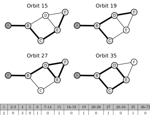
Przuljet al. [157] introducegraphlets; that are small, induced, connected, and non-isomorphic subgraphs of a large network. They also annotate the nodes of all 2- to 5-node graphlets with automorphismorbits (simply called orbits), where each automorphism orbit defines a group of nodes that are topologically symmetrical in a graphlet [156]. Thirty 2- to 5-node graphlets and their 73 automorphism orbits are illustrated in Figure 1.4. Using the automorphism orbits of graphlets, Przulj et al. [156] generalize the notion of node degree to graphlet degree: the ith _{graphlet degree of a node N is} the number of graphlets thatN touches at orbiti. With this definition, the 0th _{graphlet degree corresponds to the standard definition of node degree.} The Graphlet Degree Vector (GDV) (also known as graphlet signature) of a node is a 73-dimensional vector where each value represents the graphlet degree of the node for a particular orbit. The GDV computation for node A in Gex is illustrated in Figure 1.5. The GDV of a node represents the topological structure around a node [138]. Graphlet statistics can be used in two di↵erent ways for describing the topology of a network: (1) the number of appearances of the thirty graphlets in the network, and (2) the distributions of the graphlet degrees for each of the 73 orbits. For example, Gex contains 1 of each graphlet in {G2, G4, G5, G9, G10, G13, G16, G21}, 2 of

2-node graphlet 4-node graphlets 3-node graphlets 5-node graphlets G0 G1 G2 G3 G4 G5 G6 G7 G8 0 1 2 3 4 5 6 7 8 10 11 9 13 12 14 G9 G10 G11 G12 G13 G14 G15 G16 G17 G18 G19 G20 G21 G22 G23 G24 G25 G26 G27 G28 G29 15 16 17 18 20 21 19 22 23 25 26 24 29 30 28 27 32 31 33 34 36 37 38 35 39 42 40 41 43 44 46 48 47 45 50 49 52 53 51 54 55 57 58 56 59 61 60 63 64 62 65 67 66 68 69 70 71 72

Figure 1.4: All 2- to 5-node graphlets G0, G1, G2, . . . , G29, and their

au-tomorphism orbits 0,1, . . . ,72. Nodes belonging to the same automorphism orbit are of the same shade in each graphlet.

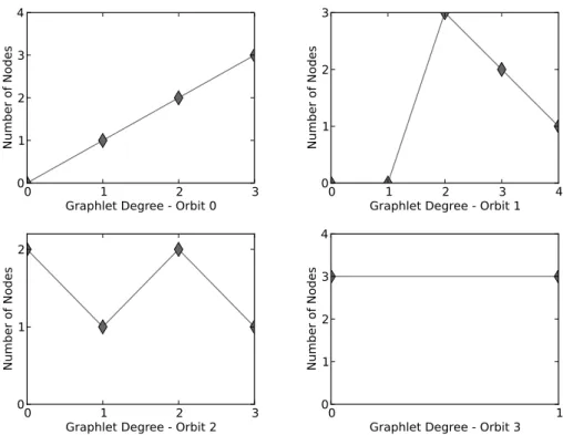
distributions of 2- and 3-node graphlet orbits (i.e., orbits 0, 1, 2, and 3) are illustrated in Figure 1.6.

In comparison to network motifs, graphlets are more powerful in captur-ing the underlycaptur-ing topology because they are defined as induced subgraphs of a network. Furthermore, they are not defined in comparison to a ran-dom network model but only on the observed counts of subgraphs, without any assumptions on a null network model. The statistics of 2- to 5-node graphlets are detailed enough to capture the topological similarities between networks, as most real-world networks are small-world networks, and 5-node graphlets capture most of their topological properties. However, the neces-sity of using 5-node graphlets is an open question that needs to be investi-gated. Furthermore, the statistics obtained from di↵erent graphlets are not completely independent of each other. There are redundancies and depen-dencies among graphlet statistics, i.e., the statistics of some graphlets can be inferred from a di↵erent set of graphlet statistics. Current graphlet-based methods [156, 157] do not handle these issues accurately, and they need to be improved further. Finally, graphlets are defined only for undirected networks, while network motifs also include directed subgraph statistics. Development of directed graphlet statistics is still an open research topic

0 1 2-3 4 5 6 7-14 15 16-18 19 20-26 27 28-34 35 36-72

1 2 0 3 0 1 0 1 0 1 0 1 0 1 0

Figure 1.5: Graphlet degree vector of node A in Gex (Figure 1.1–A) and its computation for 5-node graphlets. The number of 5-node graphlets associated with node A is 4. Notice that, the path A-B-D-F-E does not increase the graphlet degree of orbit 27, since graphlets are induced subgraphs and the induced subgraph on these nodes also contains the edge (D,E).

that is not in the scope of this dissertation.

1.4 Introduction to Network Comparison

The network comparison problem consists of three sub-problems: (1) net-work topology comparison, (2) netnet-work alignment, and (3) netnet-work query-ing. The network topology comparison problem focus on defining distance measures that evaluate the overall topological correspondence between two networks. The network alignment problem requires a more detailed com-parison that would produce a mapping between the nodes of two networks such that the correspondence between the edges of the two networks is max-imized. Finally, the network querying problem searches for a small

topolog-Figure 1.6: The graphlet degree distributions for orbits 0, 1, 2, and 3 for Gex (Figure 1.1–A). Note that, the graphlet degree distribution of orbit 0 corresponds to the degree distribution of the network (Figure 1.2–A). The topology of a network is described by the 73 graphlet degree distributions, one for each orbit in Figure 1.4.

ical pattern in a large graph. There are no polynomial-time exact solutions for any of these problems because of the underlying subgraph isomorphism problem that is NP-Complete [35]. For this reason, heuristic approaches that produce approximate solutions in polynomial-time are proposed for these problems. In this dissertation, we focus on the network topology comparison problem because of its applicability on network modelling.

The simplest heuristics for the topological network comparison problem compare the global network properties of the two networks that are de-scribed in Section 1.3.2. The single-valued global network properties (i.e., average degree, average clustering coefficient, diameter) can be directly com-pared by taking their absolute di↵erence; i.e., given two global network propertiesp1 and p2, their absolute di↵erence is|p1 p2|. When the global