GENERATING EXPLORATION MISSION-3 TRAJECTORIES TO A 9:2 NRHO USING MACHINE LEARNING
A Thesis presented to
the Faculty of California Polytechnic State University, San Luis Obispo
In Partial Fulfillment
of the Requirements for the Degree Master of Science in Aerospace Engineering
by
Esteban Guzman December 2018
c 2018 Esteban Guzman ALL RIGHTS RESERVED
COMMITTEE MEMBERSHIP
TITLE: Generating Exploration Mission-3
Trajectories to a 9:2 NRHO using Machine Learning
AUTHOR: Esteban Guzman
DATE SUBMITTED: December 2018
COMMITTEE CHAIR: Eric Mehiel, Ph.D.
Professor of Aerospace Engineering
COMMITTEE MEMBER: Kira Jorgensen Abercromby, Ph.D. Professor of Aerospace Engineering
COMMITTEE MEMBER: Amelia Greig, Ph.D.
Professor of Aerospace Engineering
COMMITTEE MEMBER: Jeffrey P. Gutkowski, EG5 Deputy Branch Chief NASA Johnson Space Center
Abstract
Generating Exploration Mission-3 Trajectories to a 9:2 NRHO using Machine Learning
Esteban Guzman
The purpose of this thesis is to design a machine learning algorithm platform that provides expanded knowledge of mission availability through a launch season by im-proving trajectory resolution and introducing launch mission forecasting. The specific scenario addressed in this paper is one in which data is provided for four determin-istic translational maneuvers through a mission to a Near Rectilinear Halo Orbit (NRHO) with a 9:2 synodic frequency. Current launch availability knowledge un-der NASA’s Orion Orbit Performance Team is established by altering optimization variables associated to given reference launch epochs. This current method can be an abstract task and relies on an orbit analyst to structure a mission based off an established mission design methodology associated to the performance of Orion and NASA’s Space Launch System. Introducing a machine learning algorithm trained to construct mission scenarios within the feasible range of known trajectories reduces the required interaction of the orbit analyst by removing the needed step of optimiz-ing the orbit to fit an expected translational response required of the spacecraft. In this study, k-Nearest Neighbor and Bayesian Linear Regression successfully predicted classical orbital elements for the launch windows observed. However both algorithms had limitations due to their approaches to model fitting. Training machine learning algorithms off of classical orbital elements introduced a repetitive approach to re-constructing mission segments for different arrival opportunities through the launch window and can prove to be a viable method of launch window scan generation for future missions.
ACKNOWLEDGMENTS
I would like to thank the following people for their guidance and support through the development of this thesis.
Jeff Gutkowski, for being an excellent mentor, helping me establish my knowl-edge in mission design development, and providing me with the opportunities to make an impact through the work he presented me.
Dr Mehiel for your constant guidance through my post-graduate degree and for sharing your perspective on how to be successful in a professional environment The Orion Orbit Performance Team for helping me establish knowledge in mis-sion considerations for the Orion vehicle
Dave Lee, for providing me with launch window mission trajectories for EM-3. Kelly Smith, for providing indispensable guidance regarding machine learning applications and how it can shape my thesis.
My friends and family for helping me maintain perspective and keeping me humble.
Maima, for your constant words of encouragement and support. Thanks for making me human
TABLE OF CONTENTS Page List of Tables . . . ix List of Figures . . . x CHAPTER 1 Introduction . . . 1
1.1 Exploration Mission 3 Background . . . 1
1.2 Launch Window Knowledge . . . 3
1.2.1 Traditional Methods in Generating Launch Window Scans . . 3
1.2.2 Machine Learning as an Alternative to Generate Launch Win-dow Scans . . . 5
1.3 Outline of Thesis . . . 6
2 Background and Literature Review . . . 8
2.1 Current Numeric Methods used in Orbital Mechanics . . . 8
2.1.1 Newton-Raphson Method . . . 8
2.1.2 Extended Kalman Filter . . . 9
2.1.3 SNOPTA . . . 10
2.1.4 Orbital Trajectory Design and Optimization Platform . . . 11
2.2 Applying Machine Learning in Orbital Mechanics . . . 12
2.2.1 Orbit Determination in LEO . . . 13
2.2.2 Modeling Circumbinary Orbit Stability . . . 13
2.2.3 Modeling an Earth to Mars Trajectory . . . 14
2.2.4 Modeling a Mission to an Asteroid Belt . . . 15
2.3 Machine Learning Approaches Considered in this Study . . . 15
2.3.1 k-Nearest Neighbor . . . 16
2.3.2 Bayesian Linear Regression . . . 19
2.4 Impact of Machine Learning in Mission Design . . . 21
3 Approach . . . 22
3.1 Mission Design Methodology . . . 22
3.1.2 Orbital Parameters in Orion Body Fixed-Moon Centered
Iner-tial Frame . . . 23
3.1.3 Suboptimal Control Thrust Parameters . . . 25
3.1.4 Key Mission Events . . . 26
3.1.5 Existing Mission Availability Scan . . . 28
3.2 Incorporating ML Algorithms for Mission Trajectory Generation . . . 28
3.2.1 Filtering Data Using Piecewise Linear Boundaries . . . 29
3.2.2 Filtering Mission Data for Machine Learning . . . 30
3.2.3 Time Scale Considerations during Training Step . . . 32
3.2.4 Preprocessing Data . . . 33
3.2.5 Computational Trajectory Generation . . . 39
4 Results . . . 42
4.1 Machine Learning Trends at each Time Step through the Mission . . 43
4.1.1 k-Nearest Neighbors . . . 43
4.1.2 Bayesian Linear Regression . . . 46
4.2 Improving Resolution for Mission Availability Scans . . . 49
4.2.1 k-Nearest Neighbor through the Launch Window . . . 50
4.2.2 Bayesian Linear Regression through the Launch Window . . . 52
4.3 Consolidating ML Projections to Construct a Trajectory . . . 54
4.4 Overall Performance of Machine Learning . . . 58
5 Analysis . . . 59
5.1 Capturing Performance through Mean Square Error . . . 59
5.2 Reliability of ML Algorithm in Reconstructing COEs . . . 60
5.2.1 Reliably Capturing COEs through Uniform Launch Epochs . . 60
5.2.2 Regions of Confident Performance . . . 62
5.3 Performance Considerations for ML Algorithms . . . 64
5.3.1 ML Model Fidelity vs Training Resolution . . . 65
5.3.2 Machine Learning Performance versus Model Configuration . . 67
5.3.3 Machine Learning Performance through the Launch Window . 70 5.4 Practical Application of ML during Mission Design . . . 70
6 Future Work . . . 73
6.1.1 Modifying the Search Radius for k-Nearest Neighbors . . . 74
6.1.2 Automatically Picking Configuration Parameters . . . 75
6.1.3 Improving Computational Demand . . . 76
6.2 Alternative Machine Learning Applications to Launch Window Con-struction . . . 77
6.3 Applying Methodology to Other Missions . . . 78
7 Conclusion . . . 80
BIBLIOGRAPHY . . . 81
APPENDICES A k-Nearest Neighbor Time Step Regression Figures . . . 83
List of Tables
Table Page
List of Figures
Figure Page
1.1 EM 3 Trajectory Overview . . . 1
1.2 NRHO Comparisons . . . 2
1.3 Traditional Method for Launch Window Scan Generation . . . 4
1.4 Machine Learning in Launch Window Scan Generation . . . 5
3.1 Family of Rendezvous with a 9:2 NRHO . . . 22
3.2 COEs for Reference Launch Epochs during Pre-OPF . . . 24
3.3 COEs for Reference Launch Epochs during NRHO . . . 25
3.4 SOC Angles wrt to the VUW Frame . . . 26
3.5 Linear Piecewise Boundary . . . 29
3.6 Training Data by Segment Nodes vs Entire Mission . . . 33
3.7 Argument of periapsis Before Pre-Processing . . . 35
3.8 Argument of periapsis After Pre-Processing . . . 36
3.9 RAAN Before Pre-Processing . . . 37
3.10 RAAN After Pre-Processing: Unwrap . . . 37
3.11 RAAN After Pre-Processing: Sine . . . 38
3.12 Scaling Perifocal Distance . . . 39
3.13 Trajectory Generation Flow Chart . . . 41
4.1 k-NN Regression Fit for Perifocal Distance through Mission . . . . 44
4.2 k-NN Regression Fit for Perifocal Distance through Pre-OPF . . . . 45
4.3 Bayesian Regression Fit for Perifocal Distance through Mission . . 46
4.4 Bayesian Regression Fit for Argument of periapsis through Out-bound Powered Flyby . . . 47
4.5 Bayesian Regression Fit for Argument of periapsis through the Pre-OPF Coast . . . 48
4.6 k-Nearest Neighbors Regression fit for Perifocal Distance through the Launch Window . . . 50
4.7 k-Nearest Neighbors Regression fit for Perifocal Distance before and after the NRHO . . . 51
4.8 Bayesian Linear Regression fit for Perifocal Distance through the
Launch Window . . . 52
4.9 Bayesian Linear Regression fit for Perifocal Distance before and after the NRHO . . . 53
4.10 k-Nearest Neighbor Model at a Time Step . . . 54
4.11 k-Nearest Neighbor Model through Mission . . . 55
4.12 Trajectory Generated by k-Nearest Neighbors . . . 56
4.13 Bayesian Regression Model at a Time Step . . . 57
4.14 Bayesian Regression Model through Mission . . . 57
4.15 Trajectory Generated by Bayesian Regression . . . 58
5.1 Non-uniform Training Distribution . . . 61
5.2 Uniform Training Distribution . . . 62
5.3 Regions of Reliability for k-Nearest Neighbor . . . 63
5.4 Regions of Reliability for Bayesian Regression . . . 64
5.5 k-Nearest Neighbor Mean Square Error . . . 66
5.6 Bayesian Regression Mean Square Error . . . 67
5.7 Number of Neighbors versus k-NN MSE . . . 68
5.8 k-Nearest Neighbors with 7 Neighbors . . . 68
5.9 Number of Samples versus Bayesian Regression MSE . . . 69
6.1 Arrival Opportunities at the NRHO versus Launch Epochs . . . 78
6.2 Perifocal Distance versus Arrival and Departure Opportunities . . . 79
A.1 k-Nearest Neighbors Fit for Eccentricity through Mission . . . 83
A.2 k-Nearest Neighbors Fit for Inclination through Mission . . . 83
A.3 k-Nearest Neighbors Fit for Right Ascension through Mission . . . 84
A.4 k-Nearest Neighbors Fit for Argument of Perigee through Mission . 84 A.5 k-Nearest Neighbors Fit for Mean Anomaly through Mission . . . . 85
A.6 k-Nearest Neighbors Fit for Epoch through Mission . . . 85
A.7 k-Nearest Neighbors Fit for MET through Mission . . . 86
B.1 Bayesian Regression Fit for Eccentricity through Mission . . . 87
B.3 Bayesian Regression Fit for Right Ascension through Mission . . . 88 B.4 Bayesian Regression Fit for Argument of Perigee through Mission . 88 B.5 Bayesian Regression Fit for Mean Anomaly through Mission . . . . 89 B.6 Bayesian Regression Fit for Epoch through Mission . . . 89 B.7 Bayesian Regression Fit for MET through Mission . . . 90
Nomenclature
Descriptive Mission Parameters
COE The oscillating classical orbital elements describing the state of a spacecraft at a given position during a mission
DSG Deep Space Gateway. NASA’s staging area for future human rated exploration missions - starting with EM-3
IAU M oon An inertial reference frame relative to the center of the moon
J D Julian Date. The number of days relative to noon UTC on January 1, 4713 BC. In this study, describes the time at launch for a reference trajectory. LEO A low earth orbit is one in which a vehicle maintains an altitude between 400
and 1,000 miles about the earth’s surface
M ET The mission elapsed time for a given trajectory as an ephemeris time N RHO Near Rectilinear Halo Orbit. DSG’s trajectory about the moon
Translational Maneuvers
N RD A departure translational maneuver from the Near Rectilinear Halo Orbit N RI An insertion translational maneuver to the Near Rectilinear Halo Orbit OP F An outbound powered flyby aligning a translunar injection burn from earth
with an entry orbit at the moon
RP F A return powered flyby aligning a return trajectory from the target trajectory back to earth
Numeric Evaluation Methods
M SE Mean Square Error. A metric comparing a projected range of regression values versus the known span of training data for machine learning algorithms SN OP T Sparse Nonlinear Optimizer. A software package evaluating large-scale
non-linear optimization problems Classical Orbital Elements
µ Gravitational parameter of the primary body
Ω Right ascension of the ascending node is a horizontal measure of the ellipse’s ascending node from the vernal point
ω Argument of periapsis is the orientation of the orbital ellipse in the orbital plane from the ascending node to the periapsis
a The semimajor axis is the sum of apoapsis and periapsis divided by two e Eccentricity measures the elongation of an ellipse as compared to a reference
circle
i Inclination describes the tilt of a trajectory with respect to a reference frame M Mean anomaly describes the angle from the periapsis for the ellipse relative to
a circular orbit with the same period
T0 The epoch of the trajectory at a given step through the mission as an ephemeris time
Chapter 1 INTRODUCTION
1.1 Exploration Mission 3 Background
Exploration mission 3 is the first step in establishing the Deep Space Gate-way (DSG) in a 9:2 synodic resonance near rectilinear halo orbit. Figure 1.1 below illustrates key mission events between launch from earth, achieving the target tra-jectory, and return to earth. Near rectilinear halo orbits are quasi-stable in nature. As a result, station keeping is relatively cheap at 254 mm/s over the span of 500 revolutions for a 9:2 NRHO. These values and further reasoning for selection of the 9:2 NRHO as the target trajectory for DSG come from a study observing cislunar exploration trajectories in reference [1].
Figure 1.1: EM 3 Trajectory Overview
A 9:2 near rectilinear halo orbit is one in which nine NRHO orbits are completed over the span of two lunar months. At a 9:2 resonance, perilune for the 9:2 NRHO is 3200 kilometers from the center of the moon as illustrated in figure 1.2.
Figure 1.2: NRHO Comparisons
The target orbit was additionally selected to mitigate loss of signal between DSG and earth. For thermal considerations of the power systems on board, the 9:2 orbit was selected to reduce the risk of being in eclipse for too long with maximum totality experienced a maximum of 1.2 hours over the span of the 20 year study completed.
The stability of the NRHO over time and distance to the moon provides easy access to a low lunar orbit or for a descent to the lunar surface. This periodicity provides a region which can be predictably targeted during rendezvous opportunities for future missions to the DSG. The Orion Multi-Purpose Crew Vehicle (MPCV) will transport crew and payloads to the DSG. Existing mission data considers the performance of the MPCV as reflected in the required duration and pointing angles for finite burns. Since this is the designed method of reaching DSG’s trajectory from EM-3 onwards (EM-3+), finite burns to enter and rendezvous with DSG in future missions consider the existing MPCV performance parameters. By examining the mission trajectory elements that comprise an insertion into this target orbit, spawned trajectories from existing data provide knowledge on what maneuvers are possible should the nominal window slip and on what maneuvers can be achieved in future
1.2 Launch Window Knowledge
Much like the mission itself, designing the trajectory profile for an explo-ration vehicle is comprised of satisfying a collection of objectives. Analysts at NASA Johnson Space Center’s Orion Performance Team employ a methodical approach to the design of mission trajectories accounting for mission objectives and vehicle con-straints. Any number of adverse conditions during launch can postpone the nominal timeline of a target mission. To account for the inevitable variability that comes with finding the ideal opportunity to launch, mission design analysts generate trajectories at defined time intervals throughout the span of a launch season. Trajectory design comes as a collaborative effort between the analyst, flight operations, and vehicle de-signers to account for required mission constraints, vehicle performance parameters, and logistical timing.
1.2.1 Traditional Methods in Generating Launch Window Scans
With all mission ground rules and assumptions applied, mission analysts generate a trajectory for a given reference launch epoch in a three degrees of freedom (3 DOF) orbital optimization platform. The established trajectory has associated with it a given cost function be it for shortest mission time, least amount of fuel con-sumed, most delta-V, etc, depending on the study performed. Launch opportunities are spawned from this nominal mission trajectory by using a wrapper script which interfaces with an informational input deck defining the mission at different intervals. The wrapper script changes the launch epoch to the desired step through the season and modifies the provided orbital parameters, treated as optimization variables, to meet the desired cost function while retaining a desired mission design methodology. The collective data package reflecting these feasible launch opportunities comprises a scan through the launch window. An overview of the traditional procedures currently
used to generate launch window scans is highlighted in figure 1.3.
Figure 1.3: Traditional Method for Launch Window Scan Generation
The process to generate said scans is computationally demanding and, as a result, time-consuming with regards to the mission analyst’s availability. The means of scripting up the wrapper code to generate the scan can also be an abstract process to generate the combination of optimization variables to satisfy the constraints of the mission for the varied time step through the launch season. By the nature of the problem, mission trajectory design is no small feat yet there exists an opportunity to alleviate the workload required to generate launch season scans by looking into alternative methods, namely machine learning.
The baseline feasibility time history values describing launch opportunities to target trajectories were treated as a training set for machine learning algorithms in this study. Pattern recognition algorithms can then impose a regression fit based off observed trends in the existing time history files. Ultimately, feasible launch trajec-tories can then be generated in keeping with the expected values from the analyzed family of solutions. The resolution of feasible trajectories can then be improved from a 1.03505 day resolution to a launch opportunity every 3 hours thus improving the resolution for potential rendezvous opportunities to the desired trajectory. The new methods incorporating machine learning are reflected in figure 1.4.
Figure 1.4: Machine Learning in Launch Window Scan Generation
1.2.2 Machine Learning as an Alternative to Generate Launch Window Scans
Machine learning is an area of study focused on automating a variety of tasks by training an algorithm to generate a desired output either by supervised or unsupervised methods. For the purposes of this study, machine learning has been employed in a pattern recognition capacity. As will be further discussed in section 2.2, machine learning can be used to fit existing trends when provided with knowledge of launch opportunities (attributes) and their related classical orbital elements (labels.) Knowledge of feasible alternative mission trajectories is then expanded by generating mission ephemeris times and COEs for different reference launch epochs. This meets the need of an orbital analyst on the Orion Performance Team who must generate high enough resolution in mission availability to support off-nominal alternative missions. For example in a scenario where weather conditions delay launch from the nominal time, generating mission trajectories through a given window provides knowledge regarding how to achieve the target trajectory for different launch times.
Machine learning algorithms do not make assumptions regarding relations between the provided attributes and labels. This provides a helpful functionality when observing unique classical orbital elements where the trends observed throughout a span of mission opportunities may not follow a single distinct pattern. In this way, machine learning provides a robust and repetitive approach to what was previously an arbitrary approach in generating launch mission scans.
1.3 Outline of Thesis
This thesis captures the design of machine learning algorithms incorporated in the generation of mission availability scans to a 9:2 NRHO. Machine learning can help alleviate the workload otherwise experienced by an orbital analyst and reduces the computational resources required when generating mission availability feasibility knowledge.
This thesis discusses the traditional numerical methods currently used when generating the orbital parameters that comprise mission trajectories. Giving an overview of machine learning will lay the ground work for effective methods in which machine learning has been incorporated through various industries. A survey of var-ious applications of machine learning in an orbital mechanics perspective will further establish why machine learning is a viable candidate for tasks considered through mission design and help validate why the decisions to use the selected ML algorithms were made. Exact explanations are provided regarding the driving mathematical con-cepts, regions of validity, and computational performance of k-Nearest Neighbor and Bayesian Linear Regression. This thesis then covers how these two models performed in aiding mission design from a machine learning performance metric perspective.
The current mission design methodology used by NASA to define transla-tional maneuvers to the moon will be discussed to give an understanding of the source data and the impact of generating trajectories using machine learning. Section 3.1 walks through what reference frames, suboptimal control pointing angles, classical orbital elements, and force model were considered in describing the desired mission trajectory and why. In section 3.2, discussion is provided on how trajectory data must be formatted when training and validating a machine learning algorithm; namely the required filtering, segregation, time-scale presentation, pre-processing steps, and
this study has been incorporated as an augmenting support function which expands on existing knowledge. Section 3.2.5 covers the steps taken when constructing a code interface to classical orbital elements and tying back code considerations to mission requirements.
Chapter 4 covers the results observed for k-Nearest Neighbor and Bayesian Linear Regression. Both models have regions of reliable performance and limitations through the epochs observed. In observing the generated data, a discussion is provided on the expected behavior of the models versus the nature of pattern fitting methods employed through the known epoch. Additional discussion is provided in chapter 5 discussing how the constructed models performed in reference to expected machine learning metrics.
Though this study has provided valuable insight into potential methods of machine learning launch window scans, there exist areas for improvement. Section 6.1 discusses how the current methods can be improved through refined model fitting methods. Other machine learning models may better suit the problem posed in this thesis so a recommendation on potential candidate models is made in section 6.2. Section 6.3 discusses how the methodology of incorporating a pattern recognition approach can be further expanded to other missions outside of the mission observed in this study.
In closing, chapter 7 contains remarks on the effectiveness of the machine learning platform constructed, how it aligns with NASA mission requirements, and how it performs in the context of machine learning.
Chapter 2
BACKGROUND AND LITERATURE REVIEW
2.1 Current Numeric Methods used in Orbital Mechanics
Understanding the dynamic interactions of exploration vehicles in a celes-tial mechanics perspective relies on numerical analysis to achieve feasible trajecto-ries. Numeric computations have aided the design of orbital trajectories throughout many different regions of astrodynamic studies. Provided with discrete observation data, numerical methods have been used in orbit determination providing analyst with a method of projecting the expected trajectory of a given spacecraft. Plane-tary stability analysis is further simulated using finite difference computations and cross comparative approaches with analytic data when considering the habitability of planets. Numeric methods support onboard guidance methods which require real time, low resource operations to understand a spacecraft’s orientation in orbit. Ve-hicle translation maneuvers are calculated with an associated cost function which reflects a performance parameter required to minimize a given metric through an in-terplanetary maneuver. For each of these scenarios, the orbital mechanics interaction is tailored to meet a mission specific operational requirement.
2.1.1 Newton-Raphson Method
The Newton-Raphson Method handles root finding by evaluating a line tan-gent to a function and extrapolating data to achieve an intersection with the x-axis. In application, Newton-Raphson has been successfully employed in initial orbital de-termination and has provided rapid convergence when observed satellite positions reflect the orbit well. Newton-Raphson provides a robust solution method capable of
determining an initial orbit through iterative refinement [2]. The Newton-Raphson method works best when the trend of the trajectory is provided with a good initial guess. As time shifts, the motion of the planetary objects considered begins to affect the feasibility of a given trajectory.
By shifting the launch epoch to the next step in the desired scan, the New-ton Raphson method becomes limited by the initial guesses provided for a family of solutions constrained to launch geodetic parameters near the initial guess. When knowledge is desired on multiple steps through a launch window, initial guesses must account for the shift in launch geodetic parameters from the nominal launch epoch. For launch opportunities where initial launch parameters shift through a launch sea-son, the initial guess posed is no longer a viable starting point and will then become computationally intensive.
2.1.2 Extended Kalman Filter
The Kalman filter is a recursive algorithm which employs a prediction and correction method in determining a desired state based off of a series of measurements with known uncertainty. Kalman filters do not require storage of prior state knowledge as the uncertainty of a range of measurements is reflected in an uncertainty matrix. Kalman filtering is common in guidance, navigation and control due to the ability to account for noise and measurement error inherent in state vector readings. The definition of the Kalman filter relies on understanding how reliable a given sensor is. Performance from a Kalman filter is additionally dependent on the complexity of the expected perturbations and dynamic models. The generated Kalman filter output can be further refined by establishing and tuning a covariance matrix over time. For a standard Kalman filter, the prediction step calculates a state transition matrix at the initial step whereas an Extended Kalman filter calculates the state transition matrix
at every time step.
In an effort to limit on-board memory storage associated to position and velocity, the author of [3] employed an Extended Kalman filter to accurately predict the attitude and orbital parameters of a spacecraft in a Molniya orbit. In this study, the author developed state matrices considering the pertubartional forces from earth’s oblateness, the moon’s gravitational force and solar radiation pressure. As more measurements are collected, the error and processing time of the state decreases. The authors of the study used readings from GPS, magnetometers, earth sensors, sun sensors, and star trackers with varying degrees of accuracy. The study was successful in predicting the orbit based off of ground station tracking measurements of the satellite and sensor readings.
2.1.3 SNOPTA
The method used for the scan of missions on which this study is based uses SNOPTA [4], a Sequential Quadratic Programming system which supports optimiza-tion variables and convergence constraints for mission definioptimiza-tions. Under SNOPTA, the orbit is propagated at variable time steps and finds extrema, minimum or max-imum depending on the objective. Searching for extrema in SNOPTA is done using sequential quadratic programming - a method of minimizing a quadratic sub-problem tied to the cost function. SNOPTA is well suited to handle the linear and non-linear constraints required for patch point convergence of the mission.
Python wrapper scripts used to generate launch window scans, as they cur-rently exist, invoke SNOPTA by way of the Copernicus executable file, resolving the problem for each new reference launch epoch through the window. In line with satis-fying the cost function through SNOPTA, optimization variables are modified in the script to ensure convergence of the trajectory to within a kilometer in position and a
centimeter per second in velocity. While using SNOPTA is necessary in establishing an initial trajectory, it is the goal of this paper to find a method which can alleviate the amount of processing required by using a less computationally intensive approach while retaining the constraints and rules for the trajectory.
2.1.4 Orbital Trajectory Design and Optimization Platform
The Orion Orbit Performance Team at NASA Johnson Space Center cur-rently utilizes Copernicus, an orbit design and optimization platform when generating mission trajectories. Copernicus is a software platform with an entire catalog of tar-geting and optimization methods for minimizing cost functions, reflecting vehicle per-formance, and factoring in body-force models for planetary interactions. The exact decisions and constraints imposed when developing a mission per NASA standards is captured in Mission Design Methodology on page 22.
In Copernicus, users have the ability to select from a range of targeting and optimization solution methods. Different portions of a mission are defined in a seg-ment, an informational data object retaining values for sequence duration, orientation with respect to a reference frame, classical orbital elements in that reference frame, mass properties of the vehicle, and any other relevant mission information. Conver-gence for a given segment is defined as falling within tolerance of either an existing state or a user defined range. In order to constrain missions to predictable arrival and departure opportunities, input decks are constructed to reflect forward and backward propagating segments associated to patch points to other segments where the need arises.
2.2 Applying Machine Learning in Orbital Mechanics
Machine learning has been around since 1959 where it was first used to train a computer the game of checkers [5]. In this study, a computer stored the rules for checkers and established weights for piece movement based off of an incentivized direction based off of board position, color, and opposing piece discrimination. The model trained between 8 and 10 hours and employed a winning strategy to beat the third ranked checker’s player in America at the time. Since then, machine learning has been incorporated in a variety of industries. In the auto industry, machine learning algorithms have been incorporated to train a car to maintain lane keeping, can predict when a car will need maintenance, and is used in hands off interaction via voice recognition services[6]. With access to large patient historic data, professionals in the medical industry have began research on incorporating machine learning to determine successful treatment and medication plans[7].
As it pertains to orbital mechanics, machine learning provides the service of generating classification and regression fits. Classification in an orbital mechanics per-spective has been used to determine the type of orbit associated to repeating classical orbital elements. Regression has been applied in orbit determination, minimization of objective functions, and spacecraft orientation during maneuvers. Both methods have provided the utility of introducing robust, versatile solutions capable of handling a range of linear and non-linear regions of a trajectory while not encumbered by the burden of data bias. Where a model can fit, a model is applied which also doubles as an efficient method of computation limiting either the post-processing execution once the model is set up or the configuration of the model itself during training.
2.2.1 Orbit Determination in LEO
In a collaborative study performed between the University of Michigan Ann Arbor and NASA’s Jet Propulsion Laboratory [8], transfer learning methods were used in the orbital determination of a CubeSat in LEO. When knowing the parameters for a given spacecraft and after having established a model to fit the provided data, the learned model can be transferred over to fit a model for which prior data is provided. The study observed the Keplerian orbital elements, [A (km), e, I (deg), Ω (deg), ω (deg), M (deg)], as a feature vector for which a training model was constructed off of 3000 pass observations. The estimation was then generated for two passes.
The vector of COEs was determined using a simulated radio frequency (RF) signal for which a bias, band frequency, and sample rate were simulated by a software defined radio system. The model then serves as a classification model which can be utilized in regression and to determine sources of noise. The model constructed in the study was successful at estimating the orbital parameters despite variance in provided data. Machine learning was also effectively used to identify and classify the orbits of specific spacecraft transmissions.
2.2.2 Modeling Circumbinary Orbit Stability
In a classification sense, machine learning can be utilized to capture the stability behavior for orbiting planets described as being in Circumbinary orbits[9]. Circumbinary orbits have the complication of being on the cusp of instability per parametric relations. The approach presented in this paper provided valid regression estimates in confirming whether a given system was stable while not generating false positives of instability associated to a polynomial fit with known regions of instability. The target problem was structured as analyzing systems initially coplanar
with circular orbits. The resulting deep neural network provided better performance in accuracy, precision and memory recall when compared against the existing method of stability calculations.
2.2.3 Modeling an Earth to Mars Trajectory
A nominal mission from Earth to Mars was treated as the baseline trajec-tory in [10]. The authors of the study noted how research into machine learning applications for orbital trajectories has been limited due to the lack of available data provided by the aerospace industry. The trajectory was initially optimized using the quadratic optimization control approach and then minimized prop mass consumed by running through as a mass optimizing scheme. The data set was expanded by per-turbing orbital parameters in the nominal trajectory. From the data generated, an optimal state feedback deep network was constructed generating a relation for thrust vectoring in polar coordinates throughout the mission.
In neural networks, activation functions must be selected to incorporate weights based off of displacements from an epoch perspective. Input and output values were both processed through activation functions. Machine learning techniques can provide a better output when the input is initially normalized as was done in this study. The number of layers in a neural network define what weights and biases are attributed to a signal ultimately resulting in what will be sent into the activation function. The more refined the number of layers in a model, the higher the fidelity of the model.
When selecting the number of layers in a neural network, there is a trade-off between the accuracy of the generated parameter and the run-time of the neural network. The authors of the paper decided that the returns on accuracy for the model stopped providing added benefit after the mean square error associated to an
extra layer was within 10−4 of an MSE from a previous layer. The resulting neural network model utilized multiple network approaches in generating the different guid-ance parameters. It was found that individual parameters had better performguid-ance by incorporating unique neural network activation functions. Overall, the neural net-work system successfully constructed mission guidance parameter projections within a reasonable error.
2.2.4 Modeling a Mission to an Asteroid Belt
In a study performed as part of a orbit optimization competition [11], the European Space Agency constructed a machine learning algorithm to determine the ideal opportunity to rendezvous to an asteroid based off of a phasing hyperparame-ter. The intention of this study was to determine when a combination of asteroids produced a combined position ideal for rendezvous with multiple asteroids at a given time. To do this, a k-Nearest Neighbor algorithm was employed to calculate a eu-clidean phase indicator. The phase indicator reflected the state vectors for a cluster of asteroids at a given time thus defining the indicator in a 6-dimensional space.
Incorporating the indicator calculated by k-Nearest Neighbor provided a useful metric for reflecting how successful a given rendezvous opportunity was at fulfilling multiple objectives for a mission through use of a decision tree.
2.3 Machine Learning Approaches Considered in this Study
The scope of this study focuses on applying machine learning to improve understanding on launch window availability by spawning missions off of existing tra-jectory data through a launch season scan. In order to do so, the machine learning algorithms considered should project inferential data based off of sparse data pro-vided for multiple arrival opportunities at the NRHO for varied launch trajectories.
The two algorithms observed in this study achieve inferential projections in similar but unique ways. Both k-Nearest Neighbors and Bayesian Linear Regression are su-pervised learning methods which require analysis beyond initial exposure to the data to provide the ideal fit of an inferred guess not in the existing data set. Where they differ is how this is achieved. k-Nearest Neighbor establishes a model fit based off of weighted contributions from nearby label/attribute combinations and serves as a fit to the data. Bayesian Linear Regression projects the data set into a Gaussian prob-abilistic function and fits the data to a function based off of likelihood of recurrence from data analysis. Both were successful in generating orbital parameters for future mission availability knowledge within certain regions of epochs.
2.3.1 k-Nearest Neighbor
Overview of k-Nearest Neighbor Regression
k-Nearest Neighbor is a machine learning algorithm which produces a re-gression function estimate based off of the k nearest elements to a given epoch and label combination [12]. For a set of data (X1, Y1)...(Xn, Yn), the default estimate of a given point is generated from the regression function mn:
mn = 1 kn kn X 1 Y(i,n)(x)
where kn reflects the impact of the k nearest elements on the estimated value of a desired unknown epoch. During evaluation, distance for a given label is relative to the specific epoch under consideration. The fraction k1
n reflects the default weight as
Search Radius
The k-Nearest Neighbor algorithm utilizes a radial search pattern to either provide classification or regression of an unknown epoch inferential from a known data set. The search radius imposed in this study is euclidean. A euclidean radius has a uniform linear reference path and can be applied in this study due to the uniform reso-lution available in the reference training data. The radius used in k-Nearest Neighbor can also be constrained to a defined function when influence disbursement may not follow a linear trend. Since evaluation of the orbital parameters is generated at the time step resolution, the euclidean search radius is considered in a two-dimensional space and is defined by the following formula:
distance= q
(epochref −epochtarget)2+ (parameterref −parametertarget)2
The neighbors with the lowest evaluation of this distance are then considered when establishing weights during an inference.
Support for Different Numerical Systems
k-Nearest Neighbor is a non-parametric machine learning algorithm which means it does not make assumptions regarding the relation between an attribute and the associated label. Because of this, k-Nearest Neighbors reflects the non-linear relations that are inherent in orbital mechanics while still maintaining the effects of body forces, perturbations, signal errors, etc. Knowledge of the distribution is determined upon each evaluation since k-Nearest Neighbors produces instance based evaluations. The regression generated then fits the distribution of data observed at each step providing support for changes in the patterns observed in future time steps.
This instance based evaluation is particularly beneficial when considering the data set provided for EM-3 where values of the classical orbital element sets tend to have a larger span of differences earlier in the mission and converge to a constant range after arriving at the NRHO as is observed in figures 3.2 and 3.3.
Computational Performance Considerations
k-Nearest Neighbor is a supervised learning scheme which requires feedback to generate the best possible fit for the spread of data. Selecting too few or too many neighbors when constructing the regression can result in a model which is respectively under or over fitting the data. A model which inappropriately fits the data may capture the training points effectively but would do poorly in generating a guess in the testing or validation sets. A valuable metric in considering how well a model is performing is the misclassification error (MSE) which reflects how well selection of the number of neighbors, k, performs in capturing the trend of the data. MSE then captures the trend for how many points are valuable in constructing a model. For an understanding of what MSE looked like when reconstructing COEs in this study, see figure
Limitations of k-Nearest Neighbor
Due to the instance based evaluation employed, the regression fit generated from Nearest Neighbor provides a fit specific to the data observed. As such, k-Nearest Neighbor does not perform well in projecting attributes for points outside of the span of epochs on which knowledge is established. Instead, k-Nearest neighbor will fit the guess generated to its nearest points which can erroneously capture a trend not in keeping with the expected pattern. Because of this, regressions formed by k-Nearest Neighbors are only reliable through the known span of epochs for which
labels are provided. k-Nearest Neighbor has a gap in performance when considering forecasting of trajectories as a result.
2.3.2 Bayesian Linear Regression
With k-Nearest Neighbor lacking in performance outside of the known range of epochs, it was of interest, in this study,to find a model which had the ability to ade-quately infer posterior trends from a sparse prior information set. Bayesian regression defines predictive functions by projecting data into a multivariate Gaussian distribu-tion [13]. Fitting the data to a multivariate distribudistribu-tion then allows for the calculadistribu-tion of a probability disbursement for a distribution of attributes within the known and unknown data set. In practice, this relation provides an inferential relation to project some label (B) provided a set of attributes (D) as a function of the attributes and some vector of adjustable parameters in the model (w): P(B|D) =f(D, w)
Gaussian Probabilistic Inferential Projection
As a Gaussian distribution, the relation between the proportionality to the probability of a data set given aw, and the prior probability distribution of w, (p(w)), a predictive projection function can be defined. This inferential projection is capable of generating new values outside of the known range of data epochs. This posterior probability is defined as:
p(t|et, α, β) = Z
p(t|w, β)p(w|et, α, β)dw
whereetis the set of training points from the existing data,p(t|w, β)is the conditional distribution, and p(w|et, α, β) is the posterior distribution of the model parameters given the training points.
A helpful metric in minimizing error in the model is considering the max-imum a posteriori distribution (MAP). The MAP is the mode of the posterior dis-tribution and is established off of prior knowledge from the provided data. Given that the Bayesian regression model incorporates a maximum a posteriori estimate, the model avoids overfitting to specific data by instead matching the likelihood of an attribute given a distribution. Calculating the MAP establishes a point inference which trends towards the maximum likelihood value. The maximum likelihood value is associated to the minimum error since error is the negative log of likelihood. By the design of Bayesian inference, the projected value minimizes error while accounting for likelihood of a label given an attribute.
Because the model of projection used in Bayesian regression imposes a fit to a Gaussian distribution, the Bayesian regression algorithm also calculates a standard deviation. This standard deviation also serves as a measure of precision for the fit along the data set based off of the degree of trust in the model.
Generalized Model Fit
Due to the generic Gaussian fitting employed, the projected model fits the trend of the values by design. This may lead to value discrepancies at certain epochs when projecting values off of the trained model. The projections generated by BRR have proven effective in capturing the expected trend from the sparse classical orbital element set on which the model is trained.
Computational Demand of BRR
Initial inference of the model can be time consuming at first as BRR attempts to fit a data set to a Gaussian distribution which may not be immediately discernible. After training the model to fit Bayesian ridge, retaining the model parameters can
make for quicker evaluation in future runs. Imposing a Gaussian distribution on a sparse data set provides a generic trend which would benefit from higher precision if provided more data points. With higher data availability, future analysis would require the trade-off between available precision and runtime performance as was discussed in 2.3.1
2.4 Impact of Machine Learning in Mission Design
This thesis is structured around constructing an algorithm which will gen-erate mission trajectories through an NRHO. Orbital parameters observed at a time step resolution reflected a periodic behavior throughout different portions of the mis-sions indicating compatibility with a pattern recognition machine learning algorithm. Using supervised learning methods, a model fit can be generated to provide a re-gression evaluation unique to each orbital parameter at each time step specific to an arrival opportunity at the DSG’s NRHO trajectory. The generated orbital parame-ters are then compiled and comprise a mission trajectory, providing mission trajectory information for a launch epoch not previously present in the data set.
k-Nearest Neighbor and Bayesian Linear Regression were both selected be-cause of their support in fitting models when sparse data is provided. Both k-Nearest Neighbors and BLR are used in projecting orbital parameters for reference launch epochs provided to the code. Existing launch window knowledge is provided at a 1.03505 day interval however inferential models for launch epochs in between these regions is desired to understand off-nominal mission opportunities. Performance for the two machine learning approaches are then evaluated against common machine learning metrics with discussion on reliability given the expected evaluation regions.
Chapter 3 APPROACH
3.1 Mission Design Methodology
Training the machine learning algorithm will focus on mission segments as-sociated to the insertion, stay and departure to and from an NRHO closest to the moon within a body fixed-moon centered inertial reference frame. These portions of the mission can be seen in figure 1.1 as the region enclosed by the red dashed line. An orbit is considered thoroughly defined when the classical orbital elements, mission ephemeris time, and delta-V maneuvers required to achieve a desired trajectory are defined. Mission availability knowledge is directly improved by machine learning algo-rithms when structured together to describe reference launch epochs. The generated trajectories achieve an arrival at an NRHO within the family of known opportunities in the existing data. Different launch opportunities comprising a family of rendezvous trajectories to the NRHO are illustrated in figure 3.1 below.
3.1.1 Force Models of the 9:2 NRHO
Dynamics about the moon have been simulated as a circular restricted three body problem in a moon-centered earth-moon rotating frame. The planetary bodies considered in the design of this trajectory are the earth, moon, and sun in line with the DE421 ephemeris. DE 421 contains a fully converged solution and comes recom-mended as the ephemeris to use for lunar missions [14]. Gravity about the moon is represented using GRAIL spherical harmonic model at degree and order 8. The grav-itational parameters for the earth and sun are represented as point masses captured below in table 3.1
Body Gravitational Parameter (km3/s2)
Earth 398600.436233
Moon 4902.800076
Sun 132712440040.944
Table 3.1: NRHO Gravitational Parameters
3.1.2 Orbital Parameters in Orion Body Fixed-Moon Centered Inertial Frame
Similar to what the authors of [11] saw when attempting to rendezvous with asteroids from an ephemeris set, the orbital parameters describing the trajectory to an NRHO maintain a periodic pattern. The classical orbital elements considered in the mapping of Orion at a given point in an EM-3+ trajectory are perifocal distance, eccentricity, inclination, right ascension of the ascending node, argument of periapsis, mean anomaly, the epoch at the point in the mission, and the gravitational parameter of the primary planetary body. These elements along with the mission elapsed time as an ephemeris time are required when propagating a trajectory through an orbits software package.
Coupling the quasi-stability of the NRHO, and establishing a desired ren-dezvous phase region as described in 1.1 results in a repeating pattern for all orbital
parameters observed through a given launch season. Through the entirety of the mis-sion trajectory, the repeating patterns observed in the classical orbital elements are associated to families of arrival epochs at the NRHO. A family of arrivals comprises multiple launch opportunities that arrive at a specific rendezvous opportunity with the NRHO at its perilune.
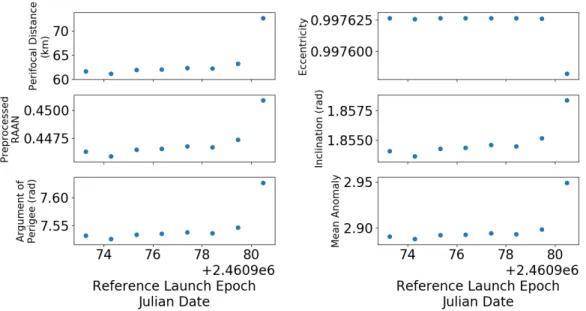
When converged in Copernicus, mission segments utilize different reference frames through the various translational maneuvers. For consistency, the orbital parameters for a given trajectory were extracted from a SPICE kernel generated in Copernicus. A SPICE kernel is a trajectory data file following the format established by NASA’s Jet Propulsion Laboratory. The classical orbital elements were in a body-fixed inertial frame relative to the center of the moon (IAU MOON). In this reference frame, orbital parameters maintained discernible trends compatible with a pattern recognition algorithm. For a visual representation of what this looks like, reference figure 3.2 where the converged data set obtained from Copernicus is plotted against different launch epochs for the Pre-OPF maneuver. Notice that each classical orbital element sets have unique patterns associated to different launch opportunities yet they all follow some distinguishable pattern.
Additionally, the classical orbital element through the stay at the NRHO, reflected in figure 3.3, maintain their own unique periodic patterns. With the COEs trending towards values related to arrival opportunities at the NRHO, it is more apparent here that the orbital parameters are converging to a fixed phase entry to the NRHO as required for a rendezvous with DSG.
Figure 3.3: COEs for Reference Launch Epochs during NRHO
3.1.3 Suboptimal Control Thrust Parameters
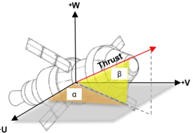
Translational maneuvers were modeled in Copernicus using sub-optimal con-trol in the VUW reference frame relative to Orion’s velocity vector. For insertion and departure burns, it is of interest to capture right ascension (α) and declination (β) to describe the in plane and out of plane angles for a translational maneuver. Right ascension and declination, illustrated in figure 3.4, describe the required orientation of the MPCV during translational maneuvers for insertion into the fixed phase ren-dezvous with DSG.
Figure 3.4: SOC Angles wrt to the VUW Frame
Angle values for each of the major translational burns are captured in the generated time history files and the machine learning algorithm trains off of the provided data in the same way a model is constructed for the orbital parameters.
3.1.4 Key Mission Events
In the design of a mission to the NRHO, NASA has maintained a methodical approach to reach the target orbit comprised of four key translational maneuvers around the moon[1]. These translational maneuvers are periods during the mission where finite burns are necessary to achieve rendezvous with the DSG orbit. The desired pattern is as follows:
• OPF an outbound powered flyby following a translunar injection maneuver from earth to align with the moon
• NRI a near rectilinear insertion burn to arrive at the NRHO • NRD a near rectilinear departure burn to leave the NRHO • RPF a return powered flyby to return to earth
Arrival and departure opportunities are made uniform when attempting to reach DSG. From an orbital mechanics perspective, it is of interest to have a pre-dictably defined region where an arrival and departure can be initiated. In the con-text of mission design, this is considered a fixed insertion phase where the position of the orbit is in line with a rendezvous opportunity with the DSG.
In the interest of capturing this rendezvous as a converged, continuous tra-jectory, the coast states between the executed finite burns are modeled as optimization variables resulting in patch points. At these patch points, position must converge for two mission segments within one kilometer for position and one cm/s for velocity. Convergence to an angle has a tolerance of +/- 0.01 degrees. The following coast segments exist throughout the span of the mission to aid in patch point convergence: • Pre-OPF a coast period aligning with a translunar injection maneuver
• Post-OPF to Pre-NRI a patch point aligning the coast state after outbound powered flyby coast state to the coast state before near rectilinear insertion finite burn
• NRHO Stay the stay period at the 9:2 near rectilinear halo orbit
• Post-NRD to Pre-RPF a patch point aligning the coast state after near recti-linear departure to the coast state before return powered flyby
A trajectory is comprised of the translational maneuvers (4) and the coast periods (6) resulting in ten segments describing a continuous trajectory to and from the NRHO. Each segment has enough nodes to reflect the position through the mission at an average of 15 second intervals.
3.1.5 Existing Mission Availability Scan
The existing mission data available for EM-3 has a baseline NRHO stay of about 5 days. Missions have been generated for a range of dates between October 2025 and November 2026 resulting in 511 unique reference launch epoch trajectories. These mission trajectories have associated with them 57 unique NRHO arrival opportunities. For a given range of reference launch epochs, a family of solutions is defined as any span of trajectories which arrive at the NRHO on a given day. Each of the trajectories for a given arrival family have associated orbital parameters describing the dynamics of Orion through an EM-3+ type mission.
3.2 Incorporating ML Algorithms for Mission Trajectory Generation
Although machine learning methods can be viable sources for recognizing patterns in data sets, the effectiveness of the model relies on how the attributes and labels are reflected numerically. For most parameters through the duration of a mis-sion, there is little work that needs to be done to capture and adequate periodic pattern. Due to the quasi-stability of the NRHO, unique families of arrival opportu-nities maintain periodicity locally. Fitting a model to the entire launch season would not adequately reflect these local patterns and would instead overfit a model through the season. Overfitting can be avoided by only considering local launch epochs which maintain the expected trend during training. Trajectories throughout the scan ex-ist where discontinuities or scaling must be resolved when training a model. The data can be pre-processed ensuring that the attribute and label relation is accurately reflected while providing a format more compatible with the algorithm considered.
3.2.1 Filtering Data Using Piecewise Linear Boundaries
When multiple families of solutions are present, a model fit must be re-strained to within a defined region using linear piecewise boundaries. Segregating data in this manner provides the benefit of generating regressions based off of rel-evant family members associated to a given distribution as reflected in figure 3.5. When used in k-Nearest Neighbor and Bayesian Linear Regression, linear piecewise boundaries confine the influence of the data to a defined region and will not erro-neously construct a trend of labels as continuous if there are multiple families of arrivals present.
Both families reflect convergence to unique trends for right ascension through the coast to outbound powered flyby. Restraining the fit to the piecewise linear bound-aries provides two unique regressions avoiding potential inaccurate fit of attributes between the region. A reference launch epoch which can align with two separate arrival opportunities must treat these scenarios separately since the local pattern is associated to the quasi-stability of the NRHO.
3.2.2 Filtering Mission Data for Machine Learning
A machine learning algorithm is only as reliable as the data it is provided because the model fit estimations treat the data provided as absolute truth; the attribute and label combination will always be true for any other observations. With a sparse data set, the impact of removing an attribute and label combination from the expected data can be significant since a model should retain as many points as possible and not erroneously negate what few data points exist. Filtering data requires a trade off between establishing an initial model fit while retaining enough data points to provide intermediate and final validation of a model. Data is filtered into three different groups when constructing a model: training, validation, and testing.
The weights and biases the machine learning algorithms produces to fit the presented data to a given model are developed during the training step. As is seen in k-Nearest Neighbors, the model directly captures the pattern of the data provided considering the impact of other data points most closely associated to a desired epoch. In Bayesian Linear Regression however, the model seeks to reflect the likelihood of a value given prior knowledge for the entire distribution. In either case, the fidelity of the generated model is directly correlated to the number of training points on which the algorithm is trained.
ex-pected trend of the data provided. Since validation data is not present during the training step, comparing the attribute and label combinations generated by the model for a given epoch versus the true value provides an unbiased comparison of just how well the data is performing. The performance of the model can be tuned by observ-ing the performance through the validation step. Validation then helps a machine learning designer understand how the number of training points used affect the hy-perparameters generated by the model without helping the model “learn."
The testing data set is a final evaluation of the fit produced by the model. Ideally, the fit should be finely tuned enough to generate an accurate estimate for the test epochs which would have not been used to establish or refine the model up to this point. If instead evaluation of the test epochs results in a discrepancy between the generated value and the truth, the model is considered to have fitting issues (see 3.2.2). Learning performance metrics generated during the testing phase describe how different hyperparameter configurations for a given model reflect the expected pattern through analysis of resulting bias and variances. Once the model meets an expected tolerance through the testing phase, it is considered ready for production and can be used to reliably infer epochs not previously present in the observed data.
Filtering Trade-Offs to Consider
An issue to keep in mind when developing a machine learning algorithm is the computational efficiency of the algorithm. After a certain amount of training data, no extra knowledge is garnered by observing extra attribute-label combinations. With no further precision generated, the machine learning algorithm can be over-encumbered in label generation for no added benefit.
Machine learning algorithms can additionally suffer from ineffective fitting when employed in pattern recognition. With too few points, the real trend of the data
provided is not accurately captured. Too many points, on the other hand, can result in overfitting of a model. A by-product of machine learning, overfitting is observed where the produced model specifically captures the label of each attribute for each epoch of the training data. Overfitting comes at the cost of losing generality of the trend and thus losing the capacity to accurately infer an epoch outside of the data set provided.
Mean square error (MSE) reflects the trade-off between the average error points for labels generated by the ML model and serves as a useful metric when determining how many data points to consider when constructing an algorithm. MSE helps the ML algorithm designer avoid overfitting by considering the bias and variance of the generated model. Overfitting is reflected in MSE as a divergence away from an otherwise converged error in bias. Selecting the number of training points to avoid inefficient processing can be done by determining when the MSE figure has converged to a given tolerance after which the model will no longer produce additional precision.
3.2.3 Time Scale Considerations during Training Step
An orbit generated using machine learning would need to follow the mission trajectory trends exhibited in the existing data. Focus must be taken to capture the scale of orbital parameters for a given segment instead of imposing comparative scales throughout the entire mission trajectory. With this in mind, a time node segment approach would provide a more effective means of replicating the mission data.
Considering a model fit at the time-step node level provides a relative com-parison of reference epochs associated to a position of a mission parallel to the position in the desired epoch. Weights and offsets generated by the function fit provided by the machine learning approach would be associated to a given time-step node rather than establishing the weights and offsets for the entire mission. In figure 3.6 below, this is
illustrated where the zoomed in segment has a more distinct shape than would have otherwise been captured by the machine learning algorithm if scaling was established for the entire trajectory.
Figure 3.6: Training Data by Segment Nodes vs Entire Mission
3.2.4 Preprocessing Data
A critical step in establishing a machine learning algorithm is presenting the data set in a format that provides an easily discernible pattern. Prior to training an algorithm, the data must be scrutinized for numeric discontinuities. Deviance of a given epoch’s attribute and label combination can reflect noise present in the analyzed signal. This study considers simulation of a given trajectory for which no signal noise exists. Data biases, such as angle phase offset, in this scenario are a byproduct of numeric processing. Without first pre-processing the data, a fit would be imposed accounting for larger differences that exist numerically but not geometrically.
Pre-processing transforms data by removing discrepancies while retaining the base geometric representation of the state captured by the attribute and label
combination. Additionally, some methods of machine learning benefit by training off of regions of data standardized to within a unity scale. In so doing, the machine learning algorithm is more effective in capturing what can otherwise be a subtle difference when comparing a span of epoch data. Specific to this study, pre-processing was employed in reshaping the classical orbital elements for compatibility with k-Nearest Neighbor and Bayesian Linear Regression. For certain angle parameters throughout the launch window, there existed angle discontinuities which required further attention to be properly reflected by a model fit. Additionally, to better support the machine learning algorithms, the orbital parameters were standardized between 0 and 1.
Angle Phase Considerations
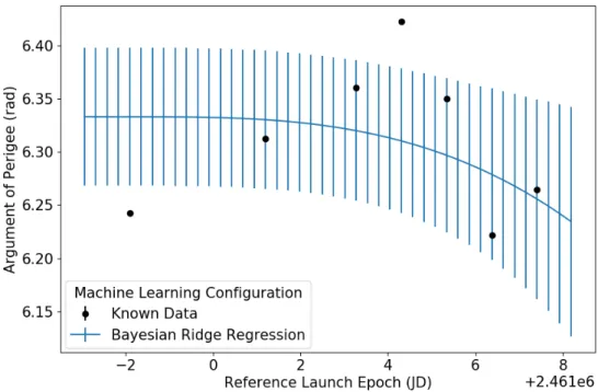
There exist phase offsets when observing some angular parameters in the classical orbital element set. While, geometrically, the values reflect the same angular displacement with respect to a given reference frame, the phase offset introduces a periodic offset. Such a phase angle shift is visible in figure 3.7 where the argument of periapsis is portrayed for a family of NRHO insertion opportunities.
Training a machine learning algorithm off of the data as it is currently re-flected would introduce a model fit to asymptotic trends. Generating an estimate from such a model introduces potential inconsistent estimates where certain time steps may reflect a deceptively large magnitude not in keeping with local epochs. The values must be processed through either unwrapping or by calculating the sine of the angle.
Figure 3.7: Argument of periapsis Before Pre-Processing
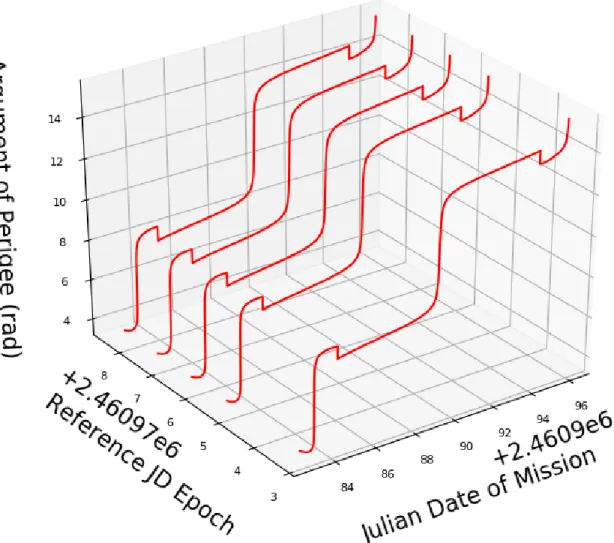
In the case for argument of periapsis, the machine learning algorithm would provide a more reliable output if it did not have to account for observable asymptotes in the data. Instead, unwrapping the angle from what would have otherwise been a value contained between 0 and 2π provides a smoother transition region among the different segments of the mission as observed in figure 3.8.
Figure 3.8: Argument of periapsis After Pre-Processing
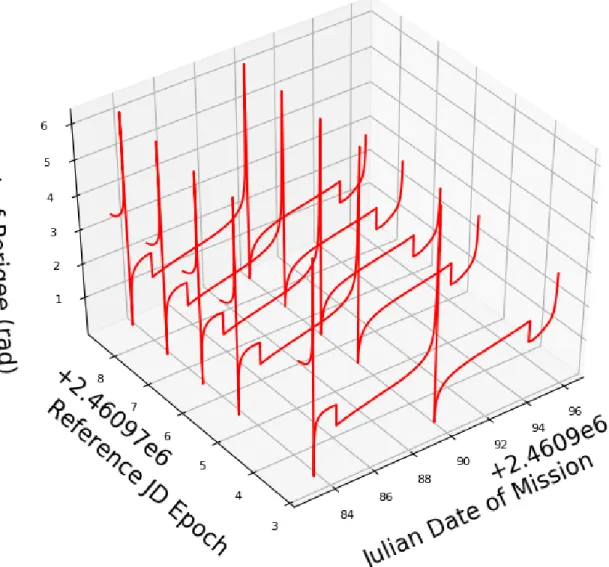
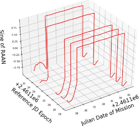
An estimate for an epoch within this trained region reflects the same angle displacement while following the expected trend when compared against local ex-pected arrival COEs. Unwrapping the angle has proven effective when constructing models for argument of periapsis, and inclination. Another orbital parameter which needs pre-processing is right ascension of the ascending node (RAAN) as seen in figure 3.9. For RAAN however, unwrapping the angle does not remove all discontinuities, as observed in figure 3.10. Instead, unwrapping the angle for RAAN introduces a different type of discontinuity.
Figure 3.9: RAAN Before Pre-Processing
Figure 3.10: RAAN After Pre-Processing: Unwrap
Rather than unwrapping the angle in the case of right ascension, the angle was pre-processed by calculating the sine of the angle, as is observed in figure 3.11. A model was then fit to the periodic value observed in the sine of RAAN, which maintained a semi-stable pattern through the NRHO. Generating the estimated value after training for the true value of right ascension was done by taking the inverse sine to revert back to an angle value.
Figure 3.11: RAAN After Pre-Processing: Sine
Scaling Time Step Values
Machine learning models can produce a better fit when the model is trained off of standardized data. Standardizing the data means transforming the incoming data between zero and one. In calculations, each parameter in a family of arrival opportunities was standardized by subtracting the minimum point observed in the time step, shifting the bias to zero. Next, all values were divided by the maximum value in the data set. An example of this is shown in figure 3.12 which shows perifocal distance, previously between approximately 180 to 375 kilometers, scaled between 0 and 1.
Figure 3.12: Scaling Perifocal Distance
By accounting for the weights and biases in the data, all labels fell within zero and one. The generated estimate from the model was then multiplied by the weight and added to the bias to regain the true parameter value of the calculation for each orbital element.
3.2.5 Computational Trajectory Generation
In this study, a mission generating script was developed using the Python [15] language. Orion’s feasible trajectories to and from the NRHO in EM-3 for an entire launch season were generated using SNOPTA in Copernicus. A python wrapper script then extracted the trajectories to a binary SPICE kernel file (BSP) which held trajectories in a spice kernel compatible format. Classical orbital elements were then generated by using the position data in the BSP files for the desired frame using SpiceyPy, a spice kernel module for python.
The COEs were generated at a defined resolution for each of the segments described in section 3.1.4. Generating the COEs with a fixed resolution ensured that each time step was relative to a fixed position in the mission for the different families of arrival opportunities considered when constructing a model fit. For example the nth element in a time history file would always be in the pre-outbound powered flyby segment of each launch opportunity through the season. The orbital elements describing were then stored in unique comma-separated value (CSV) time history files. The python script interfaced with the existing time history files by extracting classical orbital element parameters at each time step.
Piecewise linear boundaries define arrival families in the python script by extracting the arrival date at the NRHO from all of the trajectories in the launch season. Running the python script from a command prompt, the user is asked to put in a target reference epoch. Upon receiving the target epoch within the defined range, the algorithm determines which family of launch epochs the provided epoch can be compared against. There are trajectories associated to reference launch days on which a given mission can arrive at an NRHO for two separate opportunities. When facing such an opportunity, the machine learning algorithm generates both feasible trajectories and leave decision making regarding the desired NRHO insertion day to the discretion of the orbital analyst.
Once the relevant boundaries are determined for a target epoch, the python script generates a model fit for the family of arrival opportunities at each time step using machine learning algorithms. k-Nearest Neighbor and Bayesian Linear Re-gression were both incorporated using the Scikit-learn package[16] in Python. The configuration parameters for k-Nearest Neighbors and Bayesian Linear Regression were determined based off the sparsity of the data set provided and effective range of where the selected models were expected to project feasible values. The