AUDIO FEATURE EXTRACTION WITH CONVOLUTIONAL AUTOENCODERS WITH
APPLICATION TO VOICE CONVERSION
Golnoosh Elhami
´
Ecole Polytechnique F´ed´erale de Lausanne
Lausanne, Switzerland
[email protected]Romann M. Weber
Disney Research
Zurich, Switzerland
[email protected] ABSTRACTFeature extraction is a key step in many machine learning and signal processing applications. For speech signals in particular, it is impor-tant to derive features that contain both the vocal characteristics of the speaker and the content of the speech. In this paper, we intro-duce a convolutional auto-encoder (CAE) to extract features from speech represented via proposed short-time discrete cosine trans-form (STDCT). We then introduce a deep neural mapping at the encoding bottleneck to enable converting a source speaker’s speech to a target speaker’s speech while preserving the source-speech con-tent. We further compare this approach to clustering-based and lin-ear mappings.
Index Terms— Feature Extraction, Voice Conversion,
Short-Time Discrete Cosine Transformation, Convolutional Autoencoder, Deep Neural Networks, Audio Processing.
1. INTRODUCTION
The characteristics of an individual’s voice are in many ways imbued
with thecharacterof the individual. In animated entertainment
mak-ing use of human voice actors, much thought is given to the vocal performance for each character, which can become iconic, to ensure that the personality implied by the voice matches what is intended by the character’s creators. The immediately recognizable falsetto of Mickey Mouse, for one example, was originally voiced by Walt Disney himself.
Voice conversionis the problem of making a source voice sound like a target voice. It is a challenging problem for humans—very few excel at convincingly imitating the voices of others—and a still-unsolved problem in signal processing and machine learning. The challenge comes from the utter complexity of human speech, the best theoretical models for which are still gross simplifications.
Given the complexity of the speech signal, we must extract fea-tures that preserve the characteristics of the speaker and the speech signal while also significantly reducing the dimension of the prob-lem. A recent and thorough overview of how voice conversion meth-ods are traditionally approached is provided in [1].
Our approach in this work focuses on data from a parallel audio corpus—matching sentences recorded from both source and target
speakers.1 Our aim is to extract useful features first and then find a
mapping of the source-signal features to those of the target. Feature-extraction methods for voice fall into two categories: The first assumes that an excitation is passed through the vocal tract, This work was performed while the first author was at Disney Research.
1This need not be a major limitation. Furthermore, voice conversion can
effectively become voice synthesis if a synthetic test-to-speech (TTS) system is used as the source voice, in which case generating parallel data is easy.
Param. Value Module Unit Set
sample-rate 22050 Sampling – –
win-size 45 ms Win/Zdel (I)STDCT –
shift-size 12.5 ms Win/OandA (I)STDCT –
n-dct 1024 Zpad/IDCT (I)STDCT –
n-coeff 256 DCT/IDCT (I)STDCT –
n-frames 8 Concat STDCT –
n-offset 1 Concat STDCT trn
batch-size 128 – CAE trn/val
learning-rate 2e4 – CAE trn/val
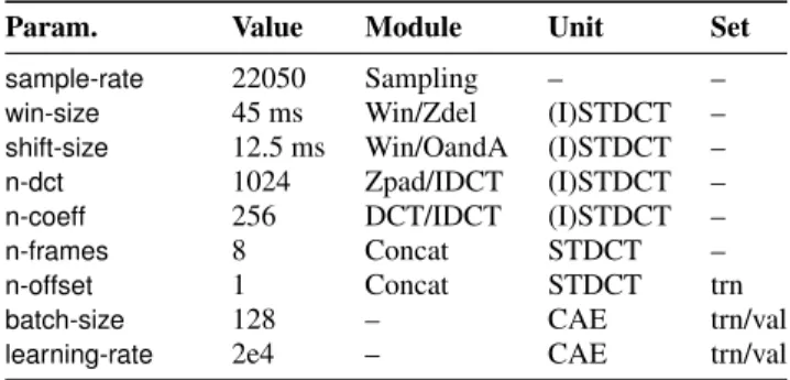
Table 1: Hyperparameters related to the FE network. Column “Set” shows if the parameter is for training (trn) or validation (val).
which is represented by a filter, and tries to extract speech features by estimating this filter [2–6]. The second drops the filter assump-tion and tries to extract features directly from the speech signal [7– 9]. The usual starting place in both approaches is the short-time Fourier transform (STFT) of the speech signal to define the features. However, as we will discuss shortly, using the STFT introduces con-straints to the system when, as is often the case, only the magnitude of the spectral data is used. In this work, we instead employ the pro-posed short-time discrete cosine transform (STDCT) of the speech signal to extract initial features.
We then introduce a deep convolutional auto-encoder (CAE) to learn nonlinear transformations of these initial features, leading to both highly compressed and high-quality representations of the speech signal. We then compare the performance of three meth-ods for mapping source representations to target representations for voice conversion—a linear transformation, clustering-based code-book method, and a deep neural network linking the source and tar-get latent spaces.
The remainder of the paper walks through the full pipeline of our method along with its complete implementation details. We then discuss and compare the proposed source-to-target voice mapping methods and present our results on a test dataset.
2. COMPRESSED FEATURE EXTRACTION
It is common in signal processing problems to reduce the complexity by extracting useful features of a signal while trying to preserve its main characteristics. To this end, signals are presented in a feature space based on their properties and the constraints of the problem at hand. For instance, wavelets are widely used for images [10]. Audio signals, on the other hand, are often transformed into a spectrogram using the short-time Fourier transform (STFT) [11–13]. In this sec-tion we take a different approach and combine several well-known
STDCT
CAE
ISTDCT
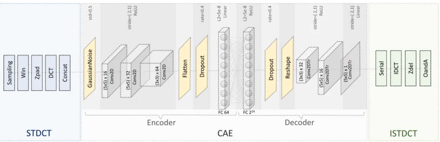
Sa m pl in g Wi n Zp ad DC T Co nc at Se ria l IDC T Oa nd A Zd el Ga ussi an N oi se Dr op ou t Fl at te n Dr op ou t Re sh ap e (5 x5 ) x 1 6 Co nv 2D (5 x5 ) x 3 2 Co nv 2D (3 x3 ) x 6 4 Co nv 2D (5 x5 ) x 1 Co nv 2D Tr (5 x5 ) x 1 6 Co nv 2D Tr (3 x3 ) x 3 2 Co nv 2D Tr FC 64 FC 214 Encoder Decoder std =0 .5 st rid e= ( 2 ,1 ) Re LU rat e= 0. 4 L2= 5e -8 Li ne ar L2= 5e -8 Re LU rat e= 0. 4 stri de =( 2 ,1 ) Re LU st rid e= ( 2 ,1 ) Li ne arFig. 1: Feature Extraction Network.
and powerful techniques to propose a new nonlinear feature space for audio signals that allows for high compression ratios on the in-put audio signal and also preserves the main characteristics of the speech.
Figure 1 shows the overall structure of our proposed
feature-extraction framework. The speech signal passes through a
pre-processing unit—labeled as STDCT here—which creates spectral samples from the audio. These samples are then fed into a deep convolutional auto-encoder (CAE) unit. The encoder transforms spectral samples into a compressed feature vector while the decoder synthesizes the spectral samples back from the encoded, compressed features. Finally, the ISTDCT unit reverts the reconstructed spectral samples into an audio signal. Details about each component of the proposed feature extraction framework are described in the reminder of this section.
2.1. Short Time Discrete Cosine Transform Unit
Many conventional techniques for extracting features of audio sig-nals utilize the STFT [1]. However, using the STFT has one major difficulty, namely that the STFT results in a complex signal that is not straightforward to work with in a neural model. Audio
classi-fication models usually only use themagnitudeof the STFT, which
discards phase information. While it is possible to produce a good reconstruction of an audio signal from spectral magnitude data alone, usually using some form of the Griffin-Lim algorithm [14], we ex-plicitly avoid this approach.
Instead, we propose to use the short-time discrete cosine trans-form (STDCT) to produce the spectral samples. This is similar to the modified discrete cosine transform (MDCT), widely used in au-dio compression techniques such as MP3 and AAC. STDCT is a time-frequency transformation formed by applying the discrete co-sine transform (DCT) [15] over windowed blocks of the audio signal. DCT has many interesting properties, but two of them are particu-larly interesting for our setting: DCT coefficients of real signals are real and DCT is a sparse representation.
The STDCT unit is shown in the left side of Figure 1. The hyper-parameters corresponding to each module and their assigned values are shown in Table 1. We first sample the input audio signal at a rate of 22050 samples per second. Then we apply a Hamming window with a length of 45 ms and shift size of 12.5 ms. We zero pad each
window to the length ofn-dct(1024 here) and take a DCT with the
same size. Since DCT is a sparse representation, we only keep the
firstn-coeffcoefficients (256 here). This operation offers us
four-times compression. In the Concat module, everyn-framesof DCT
vectors are concatenated to form a 2D input sample for the CAE
network with dimensionsn-coeff×n-frames(256×8here). For
training, an offset value ofn-offset frames is considered between
samples. In validation and testing we assume no overlap.
2.2. Convolutional Autoencoder
We use a deep convolutional autoencoder (CAE) to learn audio fea-tures from the input spectral samples. Deep convolutional autoen-coders are widely used for feature extraction in images [16] but not as often in audio processing applications. In the encoder part of the network, we use three convolutional layers to extract hierarchical features of the input spectra. The purpose of convolutional layers is to find generalizable features from the input in the form of re-curring patterns. The convolutional layers are then followed by a flattening and a fully connected layer. This layer is in charge of re-ducing the dimensionality of the input features. The decoder side of the CAE reverses this procedure and synthesizes the spectrum from the compressed features. In the proposed setup, the encoder receives
STDCT samples of size256×8as input and produces feature
vec-tors of length 64 as output. Recall that we start with STDCT samples
of size1024×8and produce feature vectors of size 64. This results
in a compression factor of 128 for the proposed feature extraction framework.
We were able to train the network successfully using only 2.5 hours of speech signal as our training set and about 10 minutes of speech signal as our validation set. We use the validation dataset to find the hyper-parameters of the network which are listed in Figure 1. In order to better generalize the network’s performance, we utilized data augmentation [17] by using a shift size of one for building train-ing samples from the STDCT spectrum and perturbtrain-ing input samples by Gaussian white noise [18]. We also added random dropout layers
andL2regularization.
2.3. Inverse Short-Time Discrete Cosine Transform Unit
In order to reconstruct the speech signal from the estimated spectral samples (the output of the decoder), we use the ISTDCT unit. Note that this unit is only used in the testing phase. Thus, the spectral samples delivered to this unit do not have any overlaps. We start by serializing the input 2D samples into the STDCT spectrum matrix. We then apply an inverse DCT on the reconstructed spectrum. This
original signal reconstructed signal
Fig. 2: An example of the original signal versus the output of CAE.
−0.05 0.00 0.05
Fig. 3: Filter coefficients in the first conv layer in the proposed CAE.
module, we keep only the firstbsample-rate×win-size×0.001cof
time samples. Finally in the OandA module, we apply “overlap and add” [19] on the frames to construct the output sequence in the time domain.
2.4. CAE Feature Extraction Results
In order to test our proposed convolutional autoencoder, we applied
the above system on the public-domain audio-bookAlice’s
Adven-tures in Wonderland.2 We chose the first 2.5 hours of the audio as training set, the next 10 minutes as validation and the remaining five minutes as test data.
In Figure 2, we show part of the original signal in blue com-pared to the reconstructed signal in orange. We can see that the au-toencoder successfully ignores the part of the signal with no speech while reconstructing the rest with high fidelity. Figure 3 shows the weights of the filters in the first convolutional layer after training. It is apparent from the figure that the network captures both low fre-quency as well as high frefre-quency information from the input spectral samples.
3. VOICE CONVERSION
In Section 2, we proposed a new method to compress speech charac-teristics into a low-dimensional feature space. These features are not only highly compressed but are also representative of speaker vo-cal characteristics and speech content. The natural question is now whether it is possible to map the speech of a source speaker onto a target speaker in this low-dimensional space. This is the essence of
voice conversion.
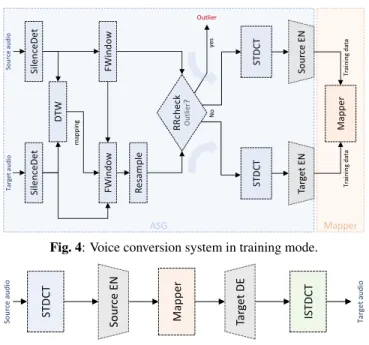
We propose a voice mapper as a solution to the voice conversion problem in the compressed feature space. We separate the training and testing phases in Figure 4 and Figure 5, respectively. During training of the voice mapper, we need to produce matching features
of source and target speech. This procedure is done in theAligned
Sample Generation(ASG) unit, shown in Figure 4. In the following section, we describe details of this procedure before moving to the voice mapper unit.
3.1. Aligned Sample Generation Unit
The purpose of the ASG unit is to produce samples that correspond to the same part of the speech from source and target speakers.
2https://youtu.be/jJHBtOu5aX0 ASG Si le nc eD et DT W ST D CT Si le nc eD et Re sa m pl e ST D CT So ur ce E N Ta rg et E N Ma pp er FW in do w FWin do w So urc e au di o Ta rge t a ud io ma pp in g ye s Outlier Tr ai ni ng da ta RRc he ck Ou tli er ? No Tr ai ni ng da ta
Fig. 4: Voice conversion system in training mode.
ST D CT So urc e au di o Ta rge t a ud io So ur ce E N Ma pp er IS TD CT Ta rg et D E
Fig. 5: Voice conversion system in test mode.
We assume to have recordings of source and target speakers for the same speech content. We feed these two speech signals to the ASG unit. We start by detecting silent regions of the two audio sig-nals and remove the ones that are longer than a predefined parameter,
slnt(here 3 ms). Then we apply dynamic time warping (DTW) [20]
on the audio signals with a frame size ofdtw-win(here 3 ms) and
a shift size ofdtw-shift(here 1.5 ms) to find the mapping between
target and source audio frames. We use a relaxed implementation of DTW, called FastDTW [21], which searches for the correspon-dences between source and target frames only within a specific
ra-dius,dtw-radius(here 100). The output of this module is the unique
correspondence between target and source frames of sizedtw-win.
For each 256×8spectral sample of the source, we note the
start and end of the temporal signal producing the sample and find the corresponding samples in the target data using the unique DTW map constructed above. The corresponding target audio contains the
same content that produced the256×8STDCT source sample. We
now resample the selected target audio to the following number of samples,
N=b (n-frames−1)×shift-size+win-size×sample-rate×10−3c.
N is the number of temporal samples required for producing eight
overlapping frames that form an STDCT sample for target. We record the resampling ratio for producing each pair of source and
Repitition Layer Neurons Description
Input 64 – GaussianNoise – std = 0.1 BatchNormalization – – 1× Dropout – rate = 0.2 Dense 512 – BatchNormalization – – ReLU – – 3× Dropout – rate = 0.2
1× Dense 64 Activation = Linear
target spectral samples. The average resample ratioravgshows how
much faster (or slower) the source speaker speaks compared to the target speaker on average. The standard deviation of resample ratios
is also saved asrstd. In the RRcheck module, we keep the STDCT
pairionly if the resample ratiorisatisfiesri∈[ravg−2rstd, ravg+
2rstd].The rest of the samples are considered to be outliers.
Now that the source and target spectral samples are ready, source samples are passed through the source encoder and the target sam-ples are passed through target encoder, which are then trained ac-cording to Section 2.1. This results in the paired feature samples for the source and target speakers.
3.2. Voice Mapper
The Mapper unit is in charge of finding the mapping between the paired feature vectors of source and target speakers. There are sev-eral methods for modeling the mapping. Here we mention a few.
3.2.1. Linear Mapper
We can make the strong assumption that the mapping between the source and target features is a linear transformation. That is, we are
looking for a transformation matrixAsuch thatSA =T,where
Ais a64×64matrix that maps the source featuresSinto target
featuresT, with S,T ∈ RM×64and M the number of training
sample pairs. The least-squares solution for such a transformation is ˆ
A= (S>S)−1S>T. We can also assume anaffinetransformation
between spaces, the solution for which follows the same form as
above if the source matrixSis augmented with a column of ones (in
which caseAˆwould be a65×64matrix).
3.2.2. Clustering Mapper
Another approach to mapping the source audio features into target features is to construct a codebook dictionary with unique mappings between source code-words and target code-words. To this end, some of the feature vectors from the training set that are the most representative of each set would be selected to be the code-words and the corresponding link between source and target codes needs to be derived. In our application, each 64-dimensional source fea-ture vector and its paired 64-dimensional target feafea-ture vector are concatenated to form a vector of length 128. We then use an off-the-shelf k-means algorithm to cluster these 128-dimensional vectors. The number of clusters in our case is a hyper-parameter, which we set to 2000. The source code-words are defined as the first 64 ele-ments of the resulting cluster representatives and the corresponding target code-words are the remaining 64 elements of the cluster rep-resentatives.
In testing mode, for a given source feature vector, we find the
cluster with minimumL2 distance to the source feature. We then
use the constructed look-up table to identify the corresponding target feature vector.
3.2.3. Deep Neural Mapper
The mapping between feature vectors of two independent speakers is more likely to be a complex transformation that cannot be fully represented using a linear mapping. To estimate complex behaviors and conveniently model the nonlinearity of the mapping, deep neural networks (DNN) are a promising method. We utilize a deep neural network to regress the target features on the source features. The structure of our proposed DNN is detailed in Table 2. Note that the
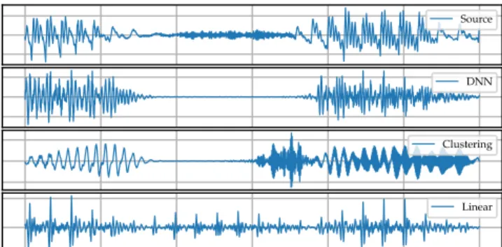
Source
DNN
Clustering
Linear
Fig. 6: Source signal compared to the converted audio for the studied mapping methods.
part of the table in blue is repeated three times as a whole, indicating a DNN with three dense hidden layers.
In order to address the potential problem of vanishing gradients [22], we add batch normalization [23] layers in the input and also before each hidden activation. Furthermore, in order to improve the generalization of the network performance, we add a Gaussian white noise layer to the input [18], as well as random dropout layers in the input and after each dense layer.
3.3. Voice Conversion Results
In order to test the performance of the above voice mappers, we trained two separate convolutional autoencoders on the audio-books ofAlice’s Adventures in Wonderland, one to represent the version narrated by a male (source) and and the other by a female (target). We then applied the above mappers on the extracted source features. Figure 6 shows a small sample of the source speech together with the transformed target speech.
In order to define a more objective metric for evaluating the
produced speech signals, we use the so-calledmel-cepstral distance
[24], defined as C(x, y) = 1 N N X k=1 20 log10kCx(k)−Cy(k)k, (1)
whereCx(k)contains the cepstral coefficients of framekof signal
x, andNis the total number of frames. The resulting mel-cepstral distance between the reconstructed target audio and the original tar-get speech is 26.36, 26.58, and 26.64 for DNN, clustering, and linear methods, respectively. Note that the distance between the original source and target speech signals is 26.80. We can see that all the studied methods improve the mel-cepstral distance. Moreover, the deep neural mapper yields the smallest distance compared to other mappers in our test.
4. CONCLUSIONS
In this work, we introduced a framework for voice conversion using source and target convolutional autoencoders operating on the short-time discrete cosine transform of audio signals. This framework re-sults in highly compressed features that carry a faithful representa-tion of the audio characteristics. We demonstrated several methods for linking the representation spaces of source and target signals. The result is a single pipeline for transforming source speech into target speech.
References
[1] S. H. Mohammadi and A. Kain, “An overview of voice
con-version systems,”Speech Communication, vol. 88, pp. 65–82,
2017.
[2] S. Imai, “Cepstral analysis synthesis on the mel frequency
scale,” inIEEE International Conference on Acoustics, Speech,
and Signal Processing, vol. 8, pp. 93–96, April 1983. [3] H. Kawahara, I. Masuda-Katsuse, and A. de Cheveign´e,
“Re-structuring speech representations using a pitch-adaptive time-frequency smoothing and an instantaneous-time-frequency-based f0 extraction: Possible role of a repetitive structure in sounds,”
Speech Communication, vol. 27, no. 3, pp. 187–207, 1999.
[4] A. Pozo,Voice Source and Duration Modelling for Voice
Con-version and Speech Repair. PhD thesis, University of Cam-bridge, 2008.
[5] E. Helander, H. Silen, T. Virtanen, and M. Gabbouj, “Voice conversion using dynamic kernel partial least squares
regres-sion,” IEEE Transactions on Audio, Speech, and Language
Processing, vol. 20, pp. 806–817, March 2012.
[6] M. I. Savic, B. Lake, S.-H. Tan, and I.-H. Nam, “Voice trans-formation system,” 1994. US Patent 5327521A.
[7] E. Moulines and F. Charpentier, “Pitch-synchronous waveform processing techniques for text-to-speech synthesis using
di-phones,”Speech Communication, vol. 9, no. 5, pp. 453–467,
1990.
[8] L. Chen, Z. Ling, L. Liu, and L. Dai, “Voice conversion us-ing deep neural networks with layer-wise generative trainus-ing,”
IEEE/ACM Transactions on Audio, Speech, and Language Processing, vol. 22, pp. 1859–1872, Dec 2014.
[9] Y. Agiomyrgiannakis, “Vocaine the vocoder and applications
in speech synthesis,” in 2015 IEEE International
Confer-ence on Acoustics, Speech and Signal Processing (ICASSP), pp. 4230–4234, April 2015.
[10] M. Vetterli and J. Kovaˇcevic,Wavelets and Subband Coding.
Upper Saddle River, NJ, USA: Prentice-Hall, Inc., 1995.
[11] T. Dutoit,An Introduction to Text-to-speech Synthesis.
Nor-well, MA, USA: Kluwer Academic Publishers, 1997.
[12] L. Wang, G. Hu, and Z. Wang, “Pitch detection based on
time-frequency analysis,” inFifth World Congress on Intelligent
Control and Automation, vol. 4, pp. 3022–3026, June 2004.
[13] H. B. Kekre, V. Kulkarni, P. Gaikar, and N. Gupta, “Ar-ticle: Speaker identification using spectrograms of varying
frame sizes,”International Journal of Computer Applications,
vol. 50, pp. 27–33, July 2012.
[14] D. Griffin and J. Lim, “Signal estimation from modified
short-time fourier transform,”IEEE Transactions on Acoustics,
Speech, and Signal Processing, vol. 32, no. 2, pp. 236–243, 1984.
[15] N. Ahmed, T. Natarajan, and K. R. Rao, “Discrete cosine
trans-form,”IEEE Transactions on Computers, vol. C–23, pp. 90–
93, Jan 1974.
[16] X. Guo, X. Liu, E. Zhu, and J. Yin, “Deep clustering with
convolutional autoencoders,” inNeural Information
Process-ing(D. Liu, S. Xie, Y. Li, D. Zhao, and E.-S. M. El-Alfy, eds.),
pp. 373–382, Springer International Publishing, 2017.
[17] K. He, X. Zhang, S. Ren, and J. Sun, “Deep residual learning
for image recognition,” inThe IEEE Conference on Computer
Vision and Pattern Recognition (CVPR), June 2016.
[18] Y. Jiang, R. M. Zur, L. L. Pesce, and K. Drukker, “A study of the effect of noise injection on the training of artificial neural
networks,” in2009 International Joint Conference on Neural
Networks, pp. 1428–1432, June 2009.
[19] L. Rabiner and B. Gold,Theory and application of digital
sig-nal processing. Prentice-Hall, 1975.
[20] D. J. Berndt and J. Clifford, “Using dynamic time warping to
find patterns in time series,” inProceedings of the 3rd
Interna-tional Conference on Knowledge Discovery and Data Mining, AAAIWS’94, pp. 359–370, 1994.
[21] S. Salvador and P. Chan, “FastDTW: Toward accurate dynamic
time warping in linear time and space,” Intell. Data Anal.,
vol. 11, no. 5, pp. 561–580, 2007.
[22] Y. Bengio, P. Simard, and P. Frasconi, “Learning long-term
de-pendencies with gradient descent is difficult,”IEEE
Transac-tions on Neural Networks, vol. 5, pp. 157–166, March 1994.
[23] S. Ioffe and C. Szegedy, “Batch normalization: Accelerating deep network training by reducing internal covariate shift,” in
International Conference on Machine Learning, pp. 448–456, 2015.
[24] R. Kubichek, “Mel-cepstral distance measure for objective
speech quality assessment,” in Proceedings of IEEE Pacific
Rim Conference on Communications Computers and Signal Processing, vol. 1, pp. 125–128, May 1993.