Research Collection School Of Information Systems
School of Information Systems
11-2016
Cost sensitive online multiple kernel classification
Doyen SAHOO
Singapore Management University, [email protected]
Peilin ZHAO
Ant Financial
Steven C. H. HOI
Singapore Management University, [email protected]
Follow this and additional works at:
https://ink.library.smu.edu.sg/sis_research
Part of the
Databases and Information Systems Commons
This Conference Proceeding Article is brought to you for free and open access by the School of Information Systems at Institutional Knowledge at Singapore Management University. It has been accepted for inclusion in Research Collection School Of Information Systems by an authorized administrator of Institutional Knowledge at Singapore Management University. For more information, please [email protected].
Citation
SAHOO, Doyen; ZHAO, Peilin; and HOI, Steven C. H.. Cost sensitive online multiple kernel classification. (2016).JMLR: Workshop and Conference Proceedings: 8th Asian Conference on Machine Learning: Hamilton, New Zealand, 2016 November 16-18. 63, 65-80. Research Collection School Of Information Systems.
Cost-Sensitive Online Multiple Kernel Classification
Doyen Sahoo [email protected]
School of Information Systems, Singapore Management University, Singapore
Peilin Zhao [email protected]
Artificial Intelligence Department, Ant Financial
Steven C.H. Hoi [email protected]
School of Information Systems, Singapore Management University, Singapore
Editors:Robert J. Durrant and Kee-Eung Kim
Abstract
Learning from data streams has been an important open research problem in the era of big data analytics. This paper investigates supervised machine learning techniques for mining data streams with application to online anomaly detection. Unlike conventional machine learning tasks, machine learning from data streams for online anomaly detection has several challenges: (i) data arriving sequentially and increasing rapidly, (ii) highly class-imbalanced distributions; and (iii) complex anomaly patterns that could evolve dy-namically. To tackle these challenges, we propose a novel Cost-Sensitive Online Multiple Kernel Classification (CSOMKC) scheme for comprehensively mining data streams and demonstrate its application to online anomaly detection. Specifically, CSOMKC learns a kernel-based cost-sensitive prediction model for imbalanced data streams in a sequential or online learning fashion, in which a pool of multiple diverse kernels is dynamically explored. The optimal kernel predictor and the multiple kernel combination are learnt together, and simultaneously class imbalance issues are addressed. We give both theoretical and extensive empirical analysis of the proposed algorithms.
Keywords: Cost-Sensitive Learning; Online Learning; Multiple Kernel Learning;
1. Introduction
With an increasing interest in mining large data streams, there is a need to design scal-able and effective learning algorithms that can comprehensively address emerging big data analytics challenges. In this paper we focus our attention on supervised learning for data streams with imbalanced labels with application to anomaly detection. Real world examples include intrusion detection (Roesch et al., 1999), anomaly detection in video surveillance (Xiang and Gong, 2008), fraud detection in markets (Donoho, 2004), and many others (Chandola et al., 2009). Despite extensive studies this remains a challenging problem due to a number of issues including: (i) high complexity (nonlinearity) of the (anomaly) pat-terns; (ii)high class-imbalanced distributions where the number of anomaly examples could be significantly less than normal ones; (iii) high variety of patterns dynamically changing due to a variety of anomaly behaviors, and high variety of data to be processed (hetero-geneous data sources, multi-modal data etc.); (iv) high volume and velocity of sequentially arriving data; and (v) pattern evolution or concept drifts.
Most existing strategies only partly address the challenges posed by imbalanced data streams, and as a result the current state of the art is not able to provide a comprehensive solution to mining imbalanced data streams or for anomaly detection. We design Cost-Sensitive Online Multiple Kernel Classification (CSOMKC) algorithms, which provide a novel method to address all the above challenges of cost-sensitive online classification (and online anomaly detection) from big data streams, including (i) highly complex patterns via kernel methods; (ii) high class imbalance via cost-sensitive learning; (iii) high variety and data heterogeneity via multiple kernel learning; (iv) high volume and velocity via online learning algorithms; as well as (v) dealing with the concept drifting via online multi-kernel learning. Designing such a technique is a significantly challenging, and would have several applications. To the best of our knowledge, this is the first learning method that can simultaneously address all these issues in a simple, efficient, scalable yet effective framework. Traditional classification algorithms aim to maximize accuracy. However, if the data exhibits imbalanced label distribution, accuracy becomes a poor measure of performance. As a result, we consider alternate metrics sum (weighted combination of specificity and sensitivity) andcost(weighted cost of misclassification of positive and negative instances) for evaluation of algorithms on imbalanced data streams. We develop a cost-sensitive multiple kernel formulation for the problem to be solved based on maximizingsumor minimizingcost and then design an online solution. We split the learning procedure in each online learning iteration - by first updating the kernel based prediction function for each of the kernels in the predefined pool (each kernel can be a different function, or different modality of data source), followed by dynamically exploring the multiple kernels, and updating the kernel combination. Both are done in an online manner, thus dealing with scalability concerns and concept drift. In addition, both the updates account for the cost-sensitive nature of the data streams. Further, we derive theoretical guarantees, and obtain the lower bound and upper bound of sum and cost respectively, obtained by our algorithms. We conduct extensive empirical analysis and show how our proposed methods outperform other state of the art cost-sensitive algorithms.
2. Related Work
Our work is primarily related to online learning and cost-sensitive learning and their inter-secting studies. Online Learning refers to a family of scalable learning methods that incre-mentally update the model from a stream of data (Cesa-Bianchi and Lugosi,2006;Hoi et al.,
2014). Many of these techniques are based on maximum-margin classification, starting from the classical Perceptron Algorithm (Rosenblatt,1958) to the more recent Online Gradient Descent (Zinkevich,2003), Relaxed Online Maximum Margin Algorithm (ROMMA) (Li and Long,2002), Approximate Maximal Margin Algorithm (ALMA) (Gentile,2002), Margin In-fused Relaxed Algorithm (MIRA) (Crammer and Singer, 2003), Passive Aggressive (PA) algorithms (Crammer et al.,2006), etc. Most of these methods do not consider imbalanced data distribution and hence are not suitable for imbalanced data streams or online anomaly detection. The most closely related work is the class of cost-sensitive online learning meth-ods that directly try to optimize over a cost-sensitive metric. These include PAUMLi et al.
(2002) which is a Perceptron based algorithm for uneven margins, cost-sensitive variant of Passive-Aggressive algorithms CPAP B (Crammer et al.,2006); and CSOC - cost-sensitive
online classification (Wang et al., 2014). There also have been some efforts in attempting to maximize the Area Under the Curve in an online manner (Zhao et al.,2011;Ding et al.,
2015). Yet, none of these methods explore how to address the complexity of data through other methods (e.g. kernels or multi-kernel solutions), thus limiting their applicability in real world settings.
Another closely related area of work is one that deals with learning with kernels. Kernel methods have shown tremendous success in detecting complex nonlinear patterns owing to their ability to induce a high-dimensional reproducible kernel Hilbert space, and learning linear patterns in this space (Sch¨olkopf and Smola, 2002). Unfortunately, there are sev-eral types of kernels, and the appropriate kernel function is not known, particularly while mining data streams where the kernel function could evolve. To address this, learning the kernel function was proposed. Some of the popular techniques include marginalized ker-nels (Kashima et al.,2003), idealized kernels (Kwok and Tsang,2003), graph-based spectral learning (Bousquet and Herrmann,2003) and non-parametric kernel learning (Zhuang et al.,
2011). Multiple Kernel Learning (MKL) (Lanckriet et al., 2004; Sonnenburg et al., 2006;
G¨onen and Alpaydın,2011) evolved as one of the most popular kernel learning technique. Many techniques have been proposed to solve the MKL optimization including SimpleMKL (Rakotomamonjy et al.,2008), Extended Level Method (Xu et al., 2008) and Mirror De-scent (Aflalo et al., 2011). Despite this MKL was plagued with computational challenges and high retraining costs. Online Learning with Kernels (Kivinen et al.,2004) and Online Multiple Kernel Learning (Jin et al., 2010;Martins et al.,2010;Hoi et al.,2013)have also been proposed to address scalability, but they do not generalize well with imbalanced data streams.
3. CSOMKC: Cost-Sensitive Online Multiple-Kernel Classification
3.1. Problem Setting
Consider a binary classification task. Here, our goal is to learn a function f : Rd → R based on a sequence of training examples D={(x1, y1), . . . ,(xT, yT)}, where xt ∈Rd is a
d-dimensional instance representing the features and yt ∈ Y ={−1,+1} is the class label
assigned to xt. We use ˆy = sign(f(x)) to predict the class assignment for any x, and
the magnitude of f(x) to measure the classification confidence. Performances of the learnt functions are usually evaluated based on accuracy A:
A=
∑T
t=1I( ˆyt=yt) T
Here I is the indicator function resulting in 1 if the condition is true, and 0 otherwise. Unfortunately, many real world datasets present imbalanced labels. For a dataset with 99% labels as−1, a model that classifies all instances as−1 has an accuracy of 99%, which prima facie seems good, but it is obviously not a good performance. Clearly, Accuracy is not a good performance indicator for (imbalanced) classification. Accordingly, for imbalanced labels, we evaluate algorithms on cost-sensitive measures: sum and cost.
Sum is the weighted sum ofsensitivityandspecificityof the algorithm. LetTp={t|yt=
+1} and Tn ={t |yt =−1} denote the set of positive and negative instances respectively.
Mp={t|yt= ˆ̸ yt; yt= +1}, and Mn ={t |yt̸= ˆyt; yt=−1} for mistakes on positive and
negative instances. Lastly, |S| denotes the number of instances in any set S. Sensitivity (Se) and Specificity (Sp) are defined as: Se = |Tp|−|M|Tp| p| and Sp = |Tn|−|M|Tn| n|. The weighted
sum parameterized byα∈[0,1] is given as:
sum=α(Se) + (1−α)(Sp)
For α= 0.5,sum is reduced to balanced accuracy.
Cost is the weighted sum of mistakes on positive and negative instances, and is param-eterized by c∈[0,1]:
cost=c(|Mp|) + (1−c)(|Mn|)
Here, the aim is to tradeoff the cost of wrongly classifying a positive instance against the cost of wrongly classifying a negative instance using tradeoff parameter c.
Our objective is to either maximize sum or minimize cost. We transform both to the following objective: min f ∑ yt=+1 ρIyˆt̸=yt + ∑ yt=−1 Iyˆt̸=yt (1) where ρ= α|Tn|
(1−α)|Tp| for maximizing sum, and ρ=
c
1−c for minimizingcost.
3.2. Cost-Sensitive Multiple Kernel Classification
Data streams may exhibit complex nonlinear patterns. Kernels have evolved as popular tools to detect nonlinearity by mapping a low dimensional feature space to a high dimensional space. We aim to learn a kernel-based prediction function to optimize the cost-sensitive measure in Eq. (1), in order to detect nonlinear patterns. We propose to use Multiple Kernel Learning (MKL) so that: (i) prior knowledge of appropriate kernel is not required; (ii) model’s learning capacity increases when multiple kernels complement each other; and (iii) heterogeneous data sources can be combined into one prediction model (e.g. using different kernels for numeric and text data, or different kernels for different modalities of data). This way we are able to learn a powerful model which can detect complex nonlinear patterns and handle a variety of data.
To do this, we first define a loss function as the convex surrogate of the indicator function (which is not convex and has been used in Eq. (1)), and we get:
ℓρ(f,(x, y)) = (ρIy=1+Iy=−1)∗max(0,1−y(f·x)) (2)
Using this loss function, Eq. (1) can be cast into the following regularized optimization (C is the regularization tradeoff parameter):
min f 1 2∥f∥ 2+C T ∑ t=1 ℓρ(f,(x, y)) (3)
Our goal is to solve this using MKL. Consider a collection of m different predefined kernel functions K = {κi : Rd×Rd → R, i = 1, . . . , m}. MKL aims to learn a
is, a weighted combination θ = (θ1, . . . , θm). The proposed cost-sensitive multiple kernel
machine can be cast into the following optimization: min θ∈∆f∈HminK(θ) 1 2∥f∥ 2 HK(θ)+C T ∑ t=1 ℓρ(f,(xt, yt)) (4) where ∆ ={θ∈Rm+ |θT1m = 1},K(θ)(·,·) = T ∑ i=1
θiκi(·,·);HK(θ)is the Reproducible Kernel
Hilbert Space induced by the multiple kernel combination; and ℓρ(f,(xi, yi)) is a convex
loss function as defined in Eq. (2). The optimization can be solved by adapting existing techniques (see section on Related Work). However, it is computationally challenging and not suitable for large data streams, and data with temporal properties. Most of the tech-niques suffer from extremely high retraining cost and expensive memory requirements. To tackle this challenge, we propose online learning based CSOMKC algorithms.
3.3. CSOMKC Algorithms
We design Cost-Sensitive Online Multiple Kernel Classification (CSOMKC), which learns the model in an online learning (hence scalable and adaptive to temporal patterns) setting. Instances are sequentially processed, and in each iteration we aim to update the kernel prediction model and the kernel combination. Doing both simultaneously in an online manner is significantly challenging, and due to imbalanced data, traditional methods can not be directly applied. We update the model via a 2-step approach: updating each kernel predictor, and updating the kernel combination.
3.3.1. Cost-Sensitive online kernel classification
We first develop a single-kernel cost-sensitive online kernel classification method. In every iteration of the online learning procedure, a kernel classifier with the prediction function
f(x) is updated by gradient descent (Kivinen et al., 2004; Wang et al., 2014) when the classifier suffers a nonzero loss. Using the cost-sensitive loss from Eq. (2) we can obtain the cost-sensitive gradient descent update by taking the derivative. The update rule for each individual kernel-based model is given by:
ft+1(x) = ft(x)−η∇fℓρt(ft,(xt, yt))
= ft(x) +ηρtytκ(xt,x)
whereρtmanages the cost-sensitivity, by settingρt=I(yt=+1)+ρI(yt=−1), andηis the
learn-ing rate parameter. At the end of each online learnlearn-ing round, we can express the prediction function as a kernel expansion (Sch¨olkopf and Smola,2002)ft+1(x) = Σti=1λiκ(xi,x) where
the λi coefficients are computed based on the update rule. For non-zero loss on the ith
instance,λi̸= 0 (the instance becomes a support vector) otherwise λi= 0.
3.3.2. Online multi-kernel combination learning
All i= 1, . . . , m kernel predictions (denoted by fti) are combined to make a final weighted prediction on each iteration:
ˆ yt= sign (∑m i=1 wti(fti(xt) ))
We propose two new cost-sensitive weight combination learning schemes: 1) Based on Exponentiated Gradient; and 2) Based on Online Gradient Descent.
EG Combination: We aim to learn the optimal cost-sensitive convex combination of
weights w= (w1, . . . , wm)⊤, where wi is set to 1/mat the beginning of the learning task. In our approach, we modify and adapt theEG algorithm (Kivinen and Warmuth,1997) to update the cost-sensitive weights. We define
ft(xt) = (ft1(xt), . . . , ftm(xt))⊤,
and formulate the rule of updating was follows:
wt+1 = arg min w∈∆DKL(w∥wt) +ηegℓ ρ(w,(f t(xt), yt)), where ∆ ={w∈Rm+ |w⊤1m = 1},DKL(u∥v) = ∑ iuiln( ui vi) is the KL-divergence.
This optimization trades off two major concerns: (i) minimizing weight distribution between new weights and old weights (measured by KL-divergence); and (ii) new weights should suffer a small loss on the instance in the current iteration. The trade-off parameter is ηeg > 0. To obtain a closed-form solution for the above optimization, we approximate
the loss function by using its first-order Taylor expansion at wt, and we get:
wt+1 = arg min w∈∆DKL(w∥wt) +ηegℓ ρ(w t,(ft(xt), yt)) +ηeg∂wℓρ(wt,(ft(xt), yt))·(w−wt) (5) For this problem, we can derive a closed-form solution as:
wt+1 =
wt⊙exp(−ηeg∇wℓρ(wt; (ft(xt), yt))
∥wt⊙exp(−ηeg∇wℓρ(wt; (ft(xt), yt))∥1
,
where⊙is element-wise product. It is easy to check that∇wℓρ(wt; (ft(xt), yt)) =−ρtytft(xt)
whenℓρ(w; (f(x), y))>0, and 0 otherwise, whereρtis set in the same manner as for learning
a single kernel predictor. We refer to this approach as CSOMKC(EG).
OGD combination: Since CSOMKC(EG) learns a convex combination, we aim to
in-crease the generality by learning the optimal cost-sensitive linear combination of multiple kernel predictors. Similar with the EG update (5), this can be cast into the following optimization: wt+1= arg min w 1 2∥w−wt∥ 2 2+ηogdℓρ(w,(ft(xt), yt))
whereft(xt) is the vector representing the predictions made by each individual kernel
clas-sifier. After replacing the loss function with its first order Taylor expansion, the update rule based on Online Gradient Descent can be derived as (Zinkevich,2003;Wang et al.,2014):
wt+1 = wt−ηogd∇wℓρ(wt,(ft(xt), yt)),
where the weights are updated only when the combined prediction suffers a loss, i.e.,
ℓρ(wt,(ft(xt), yt))>0;ηogd represents the learning rate for the weight update of the
combi-nation; and ρt regulates the update to account for cost-sensitivity. This approach referred
to as CSOMKC(OGD).
Both approaches are similar in the problem being addressed. However, EG uses multi-plicative updates, whereas OGD uses additive updates. As a result, while EG may converge to a solution faster, in the long run OGD will outperform it. Both the approaches are out-lined in Algorithm 1.
Algorithm 1 Cost-Sensitive Online Multiple Kernel Classification
INPUTS: Kernels: ki(·,·) :X × X → R, i= 1, . . . , m; Learning rates: η > 0, ηeg >0;
Cost Sensitive Parameter: ρ >0
Initialization: f1=0,w1 = m11 for t= 1,2, . . . do Receive an instance: xt Predict ˆyt= sign ( wt·ft(xt) )
Receive the class label: yt
Setρt=ρ∗I(yt= 1) +I(yt=−1) fori= 1,2, . . . , mdo Setℓρ(fti; (xt, yt)) =ρtmax(0,1−ytfti(xt)) if ℓρ(fti; (xt, yt))>0then Update fti+1(x) =fti(x) +ηiρtytκi(xt,x) end if end for Setℓρ(wt; (ft(xt), yt)) =ρtmax(0,1−ytwt·ft(xt)) if ℓρ(wt; (ft(xt), yt))>0 then
Updatewt+1 = ∥wwtt⊙⊙exp(exp(ηηegegρρttyyttfftt((xxtt))))∥1 for update by EGOR
Updatewt+1 =wt−ηogd∇wℓρ(wt,(ft(xt), yt)) for update by OGD
end if end for
3.4. Theoretical Analysis
In this section, we present the theoretical properties of the algorithm CSOMKC(EG). We derive the loss bound for Algorithm 1 when the kernel combination is learnt by EG algo-rithm. We assumeκ(x,x)≤1 for allκand x. We define the optimal regularized objective value for the kernel κi(·,·) denoted byO(κi, ℓρ,D) with respect to the datasetD as:
min fi∈Hκi ( T ∑ t=1 ℓρ(fi,(xt, yt)) +∥fi∥Hκi √ ρ2Lp i +Lni ) whereLpi =∑y t=1I(ytfi(xt)≤1), L n i = ∑ yt=−1I(ytfi(xt)≤1).
Lemma 1 Assume ∥ft(xt)∥∞≤R, and the CSOMKC(EG) algorithm is run with learning
rate ηeg =
√
2 lnm
R2T on a sequence of examples D = {(x1, y1), . . . ,(xT, yT)}. Then for any
combination of function ft= ∑m i=1wifti, w∈∆ we have T ∑ t=1 ℓρ(wt,(f(xt), yt))≤ T ∑ t=1 ℓρ(ft,(xt, yt)) +R √ Tlnm 2 . Moreover, we have ρ|Mp|+|Mn| ≤ min 1≤i≤mO(κi, ℓ ρ,D) +R √ Tlnm 2 .
Proof The idea of this proof follows the principle of similar proof in Cesa-Bianchi and Lugosi(2006). We denotelt(wt) =ℓρ(wt,(f(xt), yt)). Then, by convexity of lt, we get
lt(wt)−lt(w)≤ −(w−wt)· ∇lt(wt). (6)
Next, we would bound the right hand side of the above inequality. To facilitate the analysis, we denote z=ηeg∇lt(wt) and v=wt·z−z, then
−(w−wt)·z =−w·z+wt·z−ln( m ∑ i=1 wtievi) + ln( m ∑ i=1 witevi) =−w·z−ln( m ∑ i=1 wtie−zi) + ln( m ∑ i=1 wtievi) = m ∑ j=1 wjlne−zj−ln( m ∑ i=1 wite−zi) + ln( m ∑ i=1 witevi) = m ∑ j=1 wjln( 1 wjt wtje−zj ∑m i=1wtie−zi ) + ln( m ∑ i=1 witevi) = m ∑ j=1 wjlnw j t+1 wtj + ln( m ∑ i=1 witevi) =DKL(w∥wt)−DKL(w∥wt+1) + ln( m ∑ i=1 witevi).
Plugging the above equality into the inequality (6) and summing over t, we get
T ∑ t=1 [lt(wt)−lt(w)]≤ 1 ηeg [DKL(w∥w1) + T ∑ t=1 ln( m ∑ i=1 wtievi)],
by omitting −DKL(w∥wT+1). To bound the right hand side of the inequality, note that
DKL(w∥w1) ≤lnm, since w1 = (1/m, . . . ,1/m). We need bound the second term in the
right hand side. Since∥ft(xt)∥∞≤R, then|zi| ≤ηegR, and applying Hoeffding’s inequality:
ln( m ∑ i=1 witevi)≤η2 egR2/2.
As a result, we get the following inequality,
T ∑ t=1 [lt(wt)−lt(w)]≤ lnm ηeg +ηegR 2T 2 =R √ Tlnm 2 .
Re-arranging this concludes the first part of the theorem. If we set wi = 1 and wj = 0, for
j̸=i, usingℓρ(w
t,(ft(xt), yt))≥ρt when prediction is wrong, and combining with Lemma
1 of the paper (Wang et al.,2014), the above inequality will derive the second part.
Theorem 1 After receiving a sequence ofT training examplesD={(xt, yt), t= 1, . . . , T},
the weighted sum = α(Se) + (1−α)(Sp) achieved by Algorithm 1 for kernel combination
update by EG, withηi =∥fi∥Hκi/
√
ρ2Mp
i +Min and ρ= (1−αTαn)Tp, is bounded as:
sum≥ (1−α) Tn [ min 1≤i≤mO(κi, ℓ ρ,D) +R √ Tlnm 2 ] .
Proof We know that sum = 1− 1|T−α
n| [ α|Tn| (1−α)|Tp||Mp|+|Mn| ] . Using ρ = α|Tn| (1−α)|Tp|, and
combining the above with Lemma 1 gives us the desired result.
We now derive a bound for the cost suffered, which unlike sum does not require the estimates of ratio Tn
Tp (which may be unknown in advance). We setρ=
1−c
c , wherec∈(0,1).
Theorem 2 After receiving a sequence ofT training examplesD={(xt, yt), t= 1, . . . , T},
the weightedcost=c(|Mp|) + (1−c)(|Mn|) suffered by Algorithm 1 for kernel combiantion
update by EG, withηi =∥fi∥Hκi/
√ ρ2Mp i +Min and ρ= c 1−c, is bounded as: cost≤(1−c) [ min 1≤i≤mO(κi, ℓ ρ,D) +R √ Tlnm 2 ] .
Proof From the definition of cost, we know that cost = (1−c)(1−cc|Mp|+|Mn|) =
(1−c)(ρ|Mp|+|Mn|). Combining this with Lemma 1 proves this theorem.
Time Complexity: Traditional linear online algorithms execute inO(T) whereTis the number of instances. For an online kernel algorithm, in the worst case scenario, where every instance becomes a support vector, the algorithm would run in O(T2). However, applying budget techniques like the Randomized Budget Perceptron (Cavallanti et al.,2007) reduces the running time to O(BT) where B is the user-specified budget, and B << T. The multiple kernel variants withm kernels require time complexity of runningmonline kernel algorithms. Therefore, the time to run CSOMKC is in O(mBT), i.e., the time complexity with budget approximations is linear in number of instances.
4. Experimental Evaluation
We now present comprehensive empirical analysis of our proposed scheme, where we have evaluated algorithms’ performance on imbalanced datasets, and anomaly detection tasks.
4.1. Datasets
We use a wide variety of datasets, across a wide spectrum of applications and varying number of instances, features, and imbalance ratios. All the datasets are publicly available and were retrieved from UCI repository, LIBSVM, and KDD Cup 2008. The datasets can be categorized into 6 regular imbalanced datasets, and 2 anomaly detection datasets. Among the imbalanced datasets we have: Spam and Webspam datasets which are self
explanatory; Cod-rna is a bioinformatics dataset; Twitter dataset is about detecting buzz in social media, and is temporal in nature; Internet Ads is about predicting whether images in a given URL are ads or not; and Page-blocks attempts to classify page blocks into text or not. The anomaly detection datasets are KDD08 (from KDD Cup 2008 dataset on breast cancer); and Malware dataset built from Android Malware Genome Project which is about classifying apps as malware or not. The other details are given in Table 1.
Table 1: Details of the datasets used
Data ID Name of Dataset Instances Features Tn:T p
Regular Imbalanced Datasets
D1 Spam 4601 57 1.53 D2 Webspam 350000 254 1.54 D3 Cod-rna 59535 8 2.00 D4 Twitter 140707 77 4.07 D5 Internet Ads 3279 1556 6.14 D6 Page-blocks 21888 10 8.79
Highly Imbalanced Anomaly Detection Datasets
D7 KDD08 102294 117 163.20 D8 Malware 208243 122 549.91
4.2. Kernels
Different kernels are suitable for different types of data. For example polynomial kernels which implicitly construct new polynomial features are more suited for NLP(among other tasks). Gaussian kernels have been the most widely used kernels for a variety of tasks. Additionally, depending on the data distribution, appropriate parameters need to be set, which is often done by validation techniques. To automatically select from a rich pool of kernels, we predefine a diverse set of 10 kernels which include three polynomial kernels
κ(x, y) = (xTy)p of degree parameterp = 1,2,3,4, five RBF kernels (κ(x, y) =e(−|| x−y||2 2σ2 ))
of kernel width parameterσ = 2−2,2−1,20,21,22, and a sigmoid kernel(κ(x, y) = tanh(xy)). 4.3. Algorithms Compared
Online Learning with Kernels suffers from an unbounded growth of support vectors. For large data, even with a good classifier, the number of support vectors keeps growing linearly. To make the computation realistically possible, a budget on the number of support vectors is required. We set a budget of 2000 support vectors per kernel classifier for all datasets with number of instances greater than 50,0000, and apply the Randomized Budget Perceptron
Cavallanti et al.(2007) by randomly discarding a support vector when the budget constraint is violated, and hence approximating the kernel predictions. This approximation is done for all algorithms that make kernel based predictions. In our experiments, OMKCSC-EG and OMKCSC-OGD are compared the following algorithms:
Linear Algorithms: We compare with the following linear algorithms: 1. Simple Linear Online Gradient Descent (Zinkevich,2003)
3. CPAP B (Crammer et al.,2006) which is a cost-sensitive variant of the popular online
Passive Aggressive algorithms and
4. CSOL (Wang et al.,2014) that directly optimizes cost-sensitive measures.
Kernel Algorithms: We compare with the following online kernel methods:
1. Best Single Cost-Sensitive Kernel (CSC Kernel) determined by validation over first few samples of the data
2. Online Multiple Kernel Classification with hedge combination OMKC(H) (Hoi et al.,
2013)
3. OMKC with linear combination OMKC(OGD) (Sahoo et al.,2014)
4. Finally, we also compare with OMKCSC(U), where a uniform combination of the mul-tiple cost-sensitive kernel predictors is used, i.e., our strategies of combining mulmul-tiple kernels via EG or OGD are ignored.
All algorithms are evaluated on the basis of sum withα= 0.5 ( which is essentially the balanced accuracy); and cost with c = 0.95. For a comprehensive study, we also evaluate the results of sensitivity and specificity of each algorithm.
4.4. Parameters
There are 5 parameters required to be selected: Learning rate η for each kernel, cost-sensitive parameterρ, and the combination learning rate for EGηeg and for OGDηogd. For
a fair comparison with OMKC, we set η = 1 for all algorithms. We set the combination parameters ηeg = 0.1, and ηogd = 0.1 for all cases, and also perform sensitivity analysis
for them. The cost-sensitive parameter ρis set according to the objective being optimized. While trying to maximize sum, we set α = 0.5, and accordingly ρ is set as ρ = (1−α)Tp
αTn .
While trying to minimize the cost, we setc= 0.95, and accordinglyρ is set asρ= 1−cc.
4.5. Results and Discussion
All results are reported as the average over multiple permutations, except the Twitter dataset which is temporal in nature (random permutations are meaningless). The details are in Table 2. Further, the sum and cost of all algorithms, as the number of instances grows can be visualized in Figure1.
From Table 2, we see that our proposed CSOMKC(EG) and CSOMKC(OGD) almost
always secure the highestsum (balanced accuracy), and the lowestcost. Forsum, which in our case is a measure of balanced accuracy, CSOMKC(EG) and CSOMKC(OGD) get su-perior performances in all datasets with the exception CSOMKC(EG) in InternetAds. For the anomaly detection datasets, the proposed algorithms achieve excellent results, beat-ing the benchmarks by a significant margin. In cost performance, with the exception of CSOMKC(EG) in InternetAds, we get a significant outperformance of the proposed tech-niques in all cases. However, for all other cases, the performance is phenomenal. InternetAds has a very high dimensionality, and with the usage of multiple kernels, suffers from a rela-tively slow convergence for a small number of instances. An interesting insight can be drawn
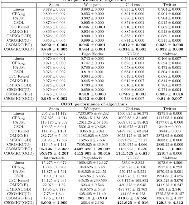
Table 2: Evaluation of all the algorithms on all datasets based on the sum and cost. SUM performance of algorithms
Spam Webspam Cod-rna Twitter Linear 0.879±0.002 0.903±0.000 0.835±0.003 0.904±0.000 CPAP B 0.809±0.002 0.853±0.000 0.801±0.000 0.901±0.000 PAUM 0.883±0.002 0.902±0.000 0.836±0.002 0.904±0.000 CSOL 0.870±0.003 0.905±0.000 0.854±0.001 0.915±0.000 CSC Kernel 0.846±0.083 0.945±0.001 0.910±0.003 0.882±0.000 OMKC(H) 0.866±0.002 0.934±0.000 0.885±0.001 0.913±0.000 OMKC(OGD) 0.825±0.008 0.900±0.000 0.863±0.002 0.889±0.000 CSOMKC(U) 0.850±0.005 0.899±0.000 0.874±0.000 0.915±0.000 CSOMKC(EG) 0.902±0.004 0.945±0.001 0.912±0.000 0.935 ±0.000 CSOMKC(OGD) 0.896±0.005 0.944±0.001 0.914±0.001 0.932 ±0.000
Internet-Ads Page-Blocks KDD08 Malware Linear 0.970±0.001 0.743±0.003 0.564±0.003 0.466±0.007 CPAP B 0.971±0.000 0.747±0.003 0.625±0.001 0.524±0.005 PAUM 0.974±0.002 0.780±0.000 0.558±0.006 0.472±0.005 CSOL 0.976±0.002 0.819±0.001 0.684±0.006 0.804±0.001 CSC Kernel 0.967±0.096 0.904±0.014 0.649±0.083 0.688±0.000 OMKC(H) 0.972±0.002 0.845±0.002 0.612±0.007 0.814±0.000 OMKC(OGD) 0.975±0.001 0.793±0.001 0.616±0.010 0.781±0.003 CSOMKC(U) 0.979±0.000 0.859±0.002 0.696±0.008 0.771±0.004 CSOMKC(EG) 0.976±0.000 0.913±0.000 0.748±0.001 0.836 ±0.018 CSOMKC(OGD) 0.985±0.002 0.912±0.001 0.733±0.007 0.84±0.007 COST performance of algorithms
Spam Webspam Cod-rna Twitter Linear 205.2±11.172 17233.975±88.282 4560.625±86.373 4275.9±0.000 CPAP B 367.625±4.914 18856.15±81.388 4002.85±31.466 4112.05±0.000 PAUM 113.175±2.369 12611.25±57.134 3669.075±55.402 4177.05±0.000 CSOL 109.35±3.041 5601.2±29.628 1349.675±3.147 2449±0.000 CSC Kernel 114.05±1.131 9055.8±3.041 2489.375±63.534 3690±0.000 OMKC(H) 282.725±5.409 11183.925±8.309 3055.125±15.167 3872.65±0.000 OMKC(OGD) 351.25±17.607 16265.4±7.637 3391.325±71.17 4883.6±0.000 CSOMKC(U) 116.45±1.131 7805.025±36.946 1950.975±4.066 2889.25±0.000 CSOMKC(EG) 95.725±3.359 4407.325±29.097 1157.225±0.530 2141 ±0.000 CSOMKC(OGD) 95.975±4.207 4412.903±30.618 1141.525±0.813 2210.7±0.000 Internet-ads Page-blocks KDD08 Malware Linear 15.275±0.672 1069.425±12.127 535.9±3.323 1973.6±4.596 CPAP B 13.45±0.849 940.525±5.48 528.975±6.116 1977.8±6.223 PAUM 11.875±1.591 848.525±22.451 550.175±5.551 1970.95±5.091 CSOL 10.9±1.344 645.85±6.435 674.975±11.208 1924.85±4.525 CSC Kernel 14.125±2.934 445.35±260.569 607.175±165.852 208.525±3.076 OMKC(H) 22.075±1.52 623.4±9.546 480.575±8.945 141.925±0.247 OMKC(OGD) 18.85±0.778 819.575±5.48 483.775±12.763 169.1±2.546 CSOMKC(U) 7.75±1.344 425.425±11.49 444.05±6.223 1725.525±2.157 CSOMKC(EG) 12.5±1.414 262.15±0.919 419.6 ±15.556 136.675±4.137 CSOMKC(OGD) 6.000±1.909 266.4±2.192 421.625±9.016 129.3 ±4.313
from1. Our proposed scheme usually picks up the best pattern, and achieves superior per-formance right from the very beginning. It is also worth noting that in some cases, single kernels give a good performance on the first few samples of the data, but eventually are not able to match OMKCSC algorithms. This demonstrates difficulty in kernel selection by validation, and hence it is imperative to have a dynamic technique that can automatically choose a combination of multiple kernels.
Linear vs Kernel Methods: The empirical results show that the introduction of kernels (and subsequently multiple kernels) have significantly increased the learning capacity of our models. In many cases, the balanced accuracy has improved by over 5% by using
kernel methods as compared to the state of the art linear models. In the optimization of cost, have caused a great reduction of the cost e.g. in the Malware dataset, the cost suffered by kernel methods is a mere 7% of the cost suffered by the best linear methods.
Comparisons between kernel methods: Among the kernel methods our proposed
techniques out performed the others, due to their ability to learn multiple cost-sensitive kernel prediction models, followed by their cost-sensitive combination. Firstly, it should be noted that the addition of multiple kernels has in fact helped increase the predictive power of the model as compared to one single kernel. However, this raises a further question: which of the algorithms CSOMKC(EG) and CSOMKC(OGD) is more suitable? CSOMKC(EG) has a a more limited predictive power as it learns only a convex combination of multiple kernels (as compared to CSOMKC(OGD). Further, if the data is described by a single kernel function, CSOMKC(EG) is able to quickly converge to that kernel predictor via multiplicative updates; but if the optimal prediction depends on a combination of several kernel functions, CSOMKC(OGD) slowly approaches the best solution, and will probably outperform CSOMKC(EG) in the long run. It should be noted that the results are very robust, as indicated by a very small standard deviation in most cases. In fact, in several cases, due to the low standard deviation, upon rounding up, it is reported as 0.
Sensitivity to learning rate parameters: We also analyzed the sensitivity of CSOMKC(EG) and CSOMKC(OGD) to their learning rates ηeg and ηogd respectively. A sample of this
analysis on the KDD08 dataset can be seen in Figure 2. As expected, both converge to the performance of OMKCSC(U) when the learning rates are set to 0. For a wide vari-ety of other learning rates, CSOMKC(EG) and CSOMKC(OGD) substantially outperform OMKCSC(U) which for the KDD08 dataset is the next best performer. CSOMKC(EG) is more robust to the parameter choice and gives consistent results across a wide range, whereas CSOMKC(OGD) gives a good performance for small values of ηogd, and when
the learning rate is very large, its performance degrades. In our experiments, we had set
ηogd = 0.1 which is a conservative choice. A carefully chosen learning rate would further
enhance the performance of CSOMKC(OGD).
5. Conclusion
In this paper, we motivated the need for scalable techniques that can learn complex non-linear patterns in imbalanced data and proposed a novel scheme of Cost-Sensitive Online Multiple Kernel Classification, which dynamically explores a diverse set of predefined kernel functions, and simultaneously learns both the kernel predictions and their optimal combi-nations. Both the kernel predictors and their combinations are learnt in a cost-sensitive manner. The kernel predictors are learnt by gradient descent, and for the kernel combi-nations, we demonstrated two approaches - first by exponentiated gradient, and second by online gradient descent. We discussed the application of the proposed techniques to online anomaly detection. We derived theoretical properties of the algorithms and have conducted extensive empirical analysis on imbalanced datasets and anomaly detection datasets. Our proposed techniques significantly outperformed several state of the art methods designed for cost-sensitive classification.
0 1000 2000 3000 4000 5000 0.4 0.5 0.6 0.7 0.8 0.9 1 T SUM Linear CPAPB PAUM CSOL Single Kernel OMKC(H) OMKC(OGD) OMKCSC(U) OMKCSC(EG) OMKCSC(OGD) (a) SUM (Spam) 0 0.5 1 1.5 2 2.5 3 3.5 x 10⁵ 0.4 0.5 0.6 0.7 0.8 0.9 1 T SUM (b) SUM (Webspam) 0 1 2 3 4 5 6 x 10⁴ 0.4 0.5 0.6 0.7 0.8 0.9 1 T SUM (c) SUM (COD-RNA) 0 5 10 15 x 104 0.4 0.5 0.6 0.7 0.8 0.9 1 T SUM (d) SUM (Twitter) 0 500 1000 1500 2000 2500 3000 3500 0.4 0.5 0.6 0.7 0.8 0.9 1 T SUM (e) SUM (InternetAds) 0 0.5 1 1.5 2 2.5 x 10⁴ 0.4 0.5 0.6 0.7 0.8 0.9 1 T SUM (f) SUM (Page-blocks) 0 2 4 6 8 10 12 x 104 0.4 0.5 0.6 0.7 0.8 0.9 1 T SUM (g) SUM (KDD08) 0 0.5 1 1.5 2 2.5 x 10⁵ 0.4 0.5 0.6 0.7 0.8 0.9 1 T SUM (h) SUM (Malware) 0 1000 2000 3000 4000 5000 0 50 100 150 200 250 300 350 400 T COST Linear CPA PB PAUM CSOL Single Kernel OMKC(H) OMKC(OGD) OMKCSC(U) OMKCSC(EG) OMKCSC(OGD) (i) COST (Spam) 0 0.5 1 1.5 2 2.5 3 3.5 x 10⁵ 0 0.2 0.4 0.6 0.8 1 1.2 1.4 1.6 1.8 2x 10 4 T COST (j) COST (Webspam) 0 1 2 3 4 5 6 x 10⁴ 0 500 1000 1500 2000 2500 3000 3500 4000 4500 5000 T COST (k) COST (COD-RNA) 0 5 10 15 x 104 0 500 1000 1500 2000 2500 3000 3500 4000 4500 5000 T COST (l) COST (Twitter) 0 500 1000 1500 2000 2500 3000 3500 0 5 10 15 20 25 T COST (m) COST (InternetAds) 0 0.5 1 1.5 2 2.5 x 10⁴ 0 200 400 600 800 1000 1200 T COST (n) COST (Page-blocks) 0 2 4 6 8 10 12 x 104 0 100 200 300 400 500 600 700 T COST (o) COST (KDD08) 0 0.5 1 1.5 2 2.5 x 10⁵ 0 200 400 600 800 1000 1200 1400 1600 1800 2000 T COST (p) COST (Malware)
Figure 1: Sum and Cost of different algorithms as the number of instances increases
0 0.2 0.4 0.6 0.8 1 0.5 0.55 0.6 0.65 0.7 0.75 0.8 0.85 0.9 0.95 1 ηeg SUM OMKCSC(U) OMKCSC(EG) (a) CSOMKC(EG) SUM 0 0.2 0.4 0.6 0.8 1 400 405 410 415 420 425 430 435 440 445 450 ηeg COST OMKCSC(U) OMKCSC(EG) (b) CSOMKC(EG) COST 0 0.02 0.04 0.06 0.08 0.1 0.12 0.14 0.16 0.5 0.55 0.6 0.65 0.7 0.75 0.8 0.85 0.9 0.95 1 ηogd SUM OMKCSC(U) OMKCSC(OGD) (c) CSOMKC(OGD) SUM 0 0.02 0.04 0.06 0.08 0.1 0.12 0.14 0.16 400 410 420 430 440 450 460 470 ηogd COST OMKCSC(U) OMKCSC(OGD) (d) CSOMKC(OGD) COST
Acknowledgements
This research is supported by the Singapore National Research Foundation under its In-ternational Research Centre @ Singapore Funding Initiative and administered by the IDM Programme Office, Media Development Authority (MDA).
References
Jonathan Aflalo, Aharon Ben-Tal, Chiranjib Bhattacharyya, Jagarlapudi Saketha Nath, and Sankaran Raman. Variable sparsity kernel learning. JMLR, 2011.
Olivier Bousquet and Daniel JL Herrmann. On the complexity of learning the kernel matrix.
Advances in NIPS, 2003.
Giovanni Cavallanti, Nicol`o Cesa-Bianchi, and Claudio Gentile. Tracking the best hyper-plane with a simple budget perceptron. Machine Learning, 2007.
Nicolo Cesa-Bianchi and Gabor Lugosi. Prediction, learning, and games. Cambridge Uni-versity Press, 2006.
Varun Chandola, Arindam Banerjee, and Vipin Kumar. Anomaly detection: A survey.
ACM Computing Surveys (CSUR), 41(3):15, 2009.
Koby Crammer and Yoram Singer. Ultraconservative online algorithms for multiclass prob-lems. JMLR, 2003.
Koby Crammer, Ofer Dekel, Joseph Keshet, Shai Shalev-Shwartz, and Yoram Singer. Online passive-aggressive algorithms. JMLR, 7:551–585, December 2006.
Yi Ding, Peilin Zhao, Steven CH Hoi, and Yew-Soon Ong. An adaptive gradient method for online auc maximization. AAAI, 2015.
Steve Donoho. Early detection of insider trading in option markets. ACM SIGKDD, 2004. Claudio Gentile. A new approximate maximal margin classification algorithm.JMLR, 2002. Mehmet G¨onen and Ethem Alpaydın. Multiple kernel learning algorithms. JMLR, 2011. Steven C.H. Hoi, Rong Jin, Peilin Zhao, and Tianbao Yang. Online multiple kernel
classi-fication. Machine Learning, 90(2):289–316, 2013.
Steven CH Hoi, Jialei Wang, and Peilin Zhao. Libol: A library for online learning algorithms. JMLR, 15:495–499, 2014.
Rong Jin, Steven C.H. Hoi, and Tianbao Yang. Online multiple kernel learning: Algorithms and mistake bounds. In Algorithmic Learning Theory. Springer Berlin Heidelberg, 2010. Hisashi Kashima, Koji Tsuda, and Akihiro Inokuchi. Marginalized kernels between labeled
J. Kivinen, A.J. Smola, and R.C. Williamson. Online learning with kernels. Signal
Process-ing, IEEE Transactions on, 52(8):2165–2176, 2004.
Jyrki Kivinen and Manfred K Warmuth. Exponentiated gradient versus gradient descent for linear predictors. Information and Computation, 132(1):1–63, 1997.
James T Kwok and Ivor W Tsang. Learning with idealized kernels. InICML, 2003. Gert R. G. Lanckriet, Nello Cristianini, Peter Bartlett, Laurent El Ghaoui, and Michael I.
Jordan. Learning the kernel matrix with semidefinite programming. JMLR, 2004. Yaoyong Li, Hugo Zaragoza, Ralf Herbrich, John Shawe-Taylor, and Jaz Kandola. The
perceptron algorithm with uneven margins. In ICML, volume 2, pages 379–386, 2002. Yi Li and Philip M Long. The relaxed online maximum margin algorithm. ML, 2002. Andr´e Martins, M Figueiredo, P Aguiar, N Smith, and E Xing. Online multiple kernel
learning for structured prediction. arXiv preprint arXiv:1010.2770, 2010.
Alain Rakotomamonjy, Francis Bach, St´ephane Canu, Yves Grandvalet, et al. Simplemkl. JMLR, 9:2491–2521, 2008.
Martin Roesch et al. Snort: Lightweight intrusion detection for networks. In LISA, vol-ume 99, pages 229–238, 1999.
Frank Rosenblatt. The perceptron: a probabilistic model for information storage and orga-nization in the brain. Psychological review, 65(6):386, 1958.
Doyen Sahoo, Steven CH Hoi, and Bin Li. Online multiple kernel regression. In ACM
SIGKDD, 2014.
Bernhard Sch¨olkopf and Alexander J Smola. Learning with kernels. The MIT Press, 2002. S¨oren Sonnenburg, Gunnar R¨atsch, Christin Sch¨afer, and Bernhard Sch¨olkopf. Large scale
multiple kernel learning. JMLR, 7:1531–1565, 2006.
Jialei Wang, Peilin Zhao, and Steven CH Hoi. Cost-sensitive online classification.Knowledge
and Data Engineering, IEEE Transactions on, 26(10):2425–2438, 2014.
Tao Xiang and Shaogang Gong. Video behavior profiling for anomaly detection. Pattern
Analysis and Machine Intelligence, IEEE Transactions on, 30(5):893–908, 2008.
Zenglin Xu, Rong Jin, Irwin King, and Michael R Lyu. An extended level method for efficient multiple kernel learning. In NIPS, pages 1825–1832, 2008.
Peilin Zhao, Rong Jin, Tianbao Yang, and Steven C Hoi. Online auc maximization. In
Proceedings of the 28th International Conference on Machine Learning (ICML-11), 2011.
Jinfeng Zhuang, Ivor W Tsang, and Steven CH Hoi. A family of simple non-parametric kernel learning algorithms. JMLR, 12:1313–1347, 2011.
Martin Zinkevich. Online convex programming and generalized infinitesimal gradient ascent. ICML, 2003.