Learning from Structured Data with High Dimensional Structured Input and Output Domain

(1)

Learning from Structured Data with High Dimensional

Structured Input and Output Domain

By

Hongliang Fei

Submitted to the graduate degree program in Electrical Engineering & Computer Science and the Graduate Faculty of the University of Kansas

in partial fulﬁllment of the requirements for the degree of Doctor of Philosophy

Committee members

Jun Huan, Chairperson

Brian Potetz

Bo Luo

Arvin Agah

Hongguo Xu

(2)

The Dissertation Committee for Hongliang Fei certiﬁes that this is the approved version of the following dissertation :

Learning from Structured Data with High Dimensional Structured Input and Output Domain

Jun Huan, Chairperson

(3)

Abstract

Structured data is accumulated rapidly in many applications, e.g. Bioinformatics, Cheminformatics, social network analysis, natural language processing and text mining. Designing and analyzing algorithms for handling these large collections of structured data has received signiﬁcant interests in data mining and machine learning communities, both in the input and output domain.

However, it is nontrivial to adopt traditional machine learning algorithms, e.g. SVM, linear regression to structured data. For one thing, the structure informa-tion in the input domain and output domain is ignored if applying the normal algorithms to structured data. For another, the major challenge in learning from many high-dimensional structured data is that input/output domain can contain tens of thousands even larger number of features and labels. With the high di-mensional structured input space and/or structured output space, learning a low dimensional and consistent structured predictive function is important for both robustness and interpretability of the model.

In this dissertation, we will present a few machine learning models that learn from the data with structured input features and structured output tasks. For learn-ing from the data with structured input features, I have developed structured sparse boosting for graph classiﬁcation, structured joint sparse PCA for anomaly detection and localization. Besides learning from structured input, I also inves-tigated the interplay between structured input and output under the context of multi-task learning. In particular, I designed a multi-task learning algorithms that performs structured feature selection & task relationship Inference. We

(4)

will demonstrate the applications of these structured models on subgraph based graph classiﬁcation, networked data stream anomaly detection/localization, mul-tiple cancer type prediction, neuron activity prediction and social behavior pre-diction. Finally, through my intern work at IBM T.J. Watson Research, I will demonstrate how to leverage structural information from mobile data (e.g. call detail record and GPS data) to derive important places from people’s daily life for transit optimization and urban planning.

(5)

Acknowledgements

I would like to express my gratitude to these faculties, colleagues and my families for their support and assistance with my dissertation.

First, I sincerely thank Dr. Jun Huan for his guidance during my graduate studies. His mentorship was great and consistent my long-term career goals. He trained me to become an independent researcher with critical thinking rather than a programmer. In reviewing my paper drafts, he offered valuable comments and insights on problem formalization and professional writing. Furthermore, he provided me with financial support for my education and conference travel. He has always taken time to introduce me to people within the discipline. I learned a lot from him, not only research skills but also his dedication towards research. I also gratefully thank my dissertation committee members: Dr. Brian Potetz, Dr. Bo Luo, Dr. Arvin Argh and Dr. Hongguo Xu. They offered professional and valuable suggestions on my proposal and dissertation.

Second, I would also like to thank all my colleagues in our research group, es-pecially Aaron Smalter, Brian Quanz and Ruoyi Jiang. These three friends and co-workers helped a lot with my research. Aaron’s code on chemical data pro-cessing and learning initialized my work in Chapter 3. Brian’s broad knowledge on machine learning and optimization further helped me to dig deeper in my dis-cipline through our discussion. Ruoyi Jiang’s creative thinking and experimental skills contributed most in Chapter 4 of my dissertation.

Third, I want to thank Dr. Ming Li, Dr. Sambit Sahu and Dr. Millind Naphade from IBM T.J. Watson Research. I appreciate their oﬀer with a platform where I

(6)

can utilize my domain knowledge in industrial problems. They gave their insights on mobility data mining and collected data sets from clients, which contributed the model and experimental design in Chapter 7. Without their help, I could not have a fulﬁlling and productive internship.

Finally but the most importantly, I want to thank my parents Haixue Fei, Qingfen Meng and two elder sisters Hongmei Fei, Hongying Fei. My parents led a very simple life to support my education from elementary school to college. Their unselﬁsh love makes me strong and warm even I stayed tens of thousands of miles away from them. My two sisters, Hongmei Fei and Hongying Fei, inspired me to have ambition and provided me with endless encouragement and support in my research and study.

(7)

6.3.3 Relationship with existing MTL algorithms . . . 106 6.3.4 Optimization . . . 107 6.4 Experimental Studies . . . 111 6.4.1 Data Sets . . . 112 6.4.2 Experiment Protocol . . . 114 6.4.3 Experiment Results . . . 115 6.4.3.1 Microarray Results . . . 115 6.4.3.2 fMRI Results . . . 119 6.4.4 Discussion . . . 121 6.5 Conclusions . . . 122

7 Leveraging Structural Information from Mobile Device Data for Meaning-ful Location Detection 123 7.1 Introduction . . . 124

7.3 Background . . . 128

7.3.1 Call Detail Record . . . 128

7.3.2 Record Data Type . . . 129

7.3.3 Tower Hopping . . . 129

7.3.4 Duration of Stay . . . 130

7.4.1 Spatial Clustering on Cell Tower Locations . . . 131

7.4.2 Duration of Stay Calculation . . . 132

7.4.3 Cluster-Zone map generation . . . 134

7.4.4 Meaningful Location Generation . . . 135

7.4.5 Home/work Detection . . . 136

7.5 Experiment . . . 136

(11)

7.5.2 Evaluation Criteria . . . 137

7.5.3 Home Work Detection Results . . . 139

7.5.4 Meaningful Location Detection Result . . . 142

7.6 Conclusion . . . 143

8 Conclusion and Future Work 145 8.1 Conclusion . . . 145

(12)

List of Figures

2.1 Examples of structured data. Top left: Protein structure data; Top right: web document data; Lower left: social network data; Lower right: gene Rb

pathway data. . . 9

2.2 An MTL example from multiple cancer prediction. . . 10

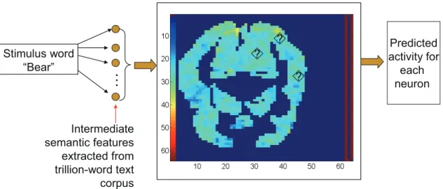
2.3 The scheme for MTL approach to neuron activity prediction: each neuron corre-sponds to a task and the features is the co-occurrence rate extracted from text corpus. “?” denotes the neuron activity value to be predicted. . . 13

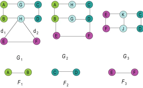
3.1 Three subgraph features in three graphs. Dashed edge means that the two nodes are connected by a path with varying length ¿1. . . 15

3.2 Accuracy comparison of on 6 data sets. . . 32

3.3 Left: Sensitivity comparison. Right: Speciﬁcity comparison . . . 33

3.4 Average accuracy with diﬀerent percentage of ﬂipped training labels . . . 35

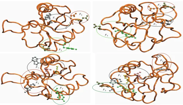
3.5 Top Left: Spatial distributions of the top 3 features from LPGBCMP in protein 1EGI. Top Right: Spatial distributions of the same 3 features from LPGBCMP in protein 1H8U. Lower Left: Spatial distributions of the top 3 features from gBoosting in protein 1EGI. Lower Right: Spatial distributions of the same 3 features from gBoosting in protein 1H8U. . . 36

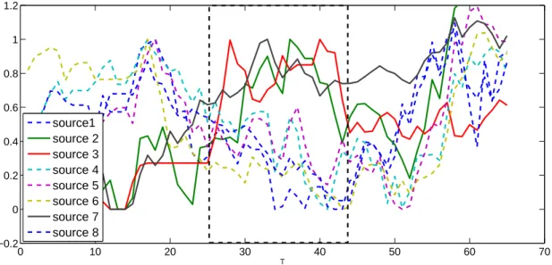
3.6 Average accuracy with diﬀerent max var . . . 37 4.1 Illustration of time-evolving stock indices data. Index 2,3,7 in solid lines are abnormal. 40

(13)

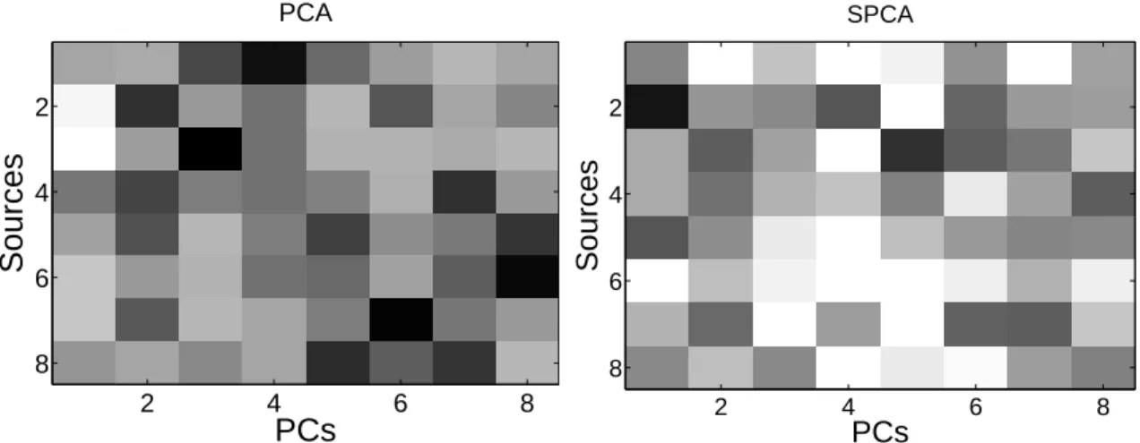
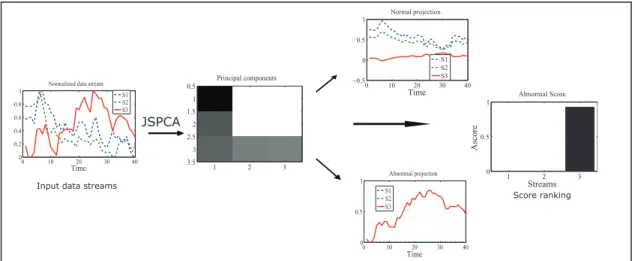
4.2 Comparing PCA and Sparse PCA. Left: PCA. Right: SPCA. . . 47 4.3 Demonstration of the the system architecture of JSPCA on three network

data streams with one anomaly (solid line) and two normal streams (dot lines). 48 4.4 Comparingjoint sparse PCA(JSPCA) andgraph joint sparse PCA(GJSPCA).

Left: JSPCA; Right: GJSPCA. . . 50 4.5 Comparing diﬀerent anomaly localization methods. From left to right: PCA, sparse

PCA, JSPCA, and GJSPCA.. . . 51 4.6 From left to right: PC space for JSKLE and GJSKLE, abnormal score for JSKLE,

and GJSKLE. . . 53 4.7 ROC curves and AUC for diﬀerent methods on three data sets. From left to right:

ROC for the stock indices data, ROC for the sensor data, ROC curve for Motor-Current data, AUC for the three ROC plots . . . 67 4.8 ROC curve for KLE extension methods on three data sets. From left to right:

ROC for the stock indices data, ROC for the sensor data, ROC curve for MotorCurrent data . . . 70 4.9 Anomaly Localization Comparison of Stochastic Nearest Neighborhood,

Eigen-Equation Compression, GJSPCA on Network Intrusion Data Set(DoS Attack) 70 4.10 Sensitivity analysis of GJSPCA on stock indices data set. From left to right: δ, the

dimension of the normal subspace,λ1 and λ2. . . 72 4.11 Sensitivity analysis of GJSKLE on stock indices data set. From left to right:δ, the

dimension of the normal subspace,λ1 and λ2. . . 73 4.12 Sensitivity analysis of GJSKLE on stock indices data set on N. . . 74 5.1 A tiny snapshot of online social network digg.com with three users. The table

(14)

5.2 Data Representation of Content Based Social Behavior Prediction. Five articles with actions of three followers and two words with tf-idf are shown for demonstration only. X is the object-feature matrix with each row representing an article and each column representing a feature. . . 83 5.3 Heterogenous social relationships betweenF1,F2 andF3 for category T: technology

and E: entertainment. Dashed line represents the technology connection and solid line represents the entertainment connection. The number for each connection represents the similarity of two users detailed in Equation 5.2. . . 83 5.4 AverageF1 score for 4 seed users. Each ﬁgure’s title corresponds to a username. . 94 6.1 A demo for the Multi-task linear model with structured input (SI) and task

rela-tionship inference (SO) with 5 features and 3 tasks. Solid line square represents input and dashed line square represents output. . . 105 6.2 Task Relationship embedding for 3 methods in 3D space from Ndaona. Left: Our

method MTLapTR; Middle: MTLPTR; Right: MTLTR . . . 117 6.3 Comparing KEGG pathway (left) and learned pathway (right) for the

Phos-phatidylinositol signaling pathway. Solid lines represent edges from KEGG and dashed lines represents additional edges learned from our algorithm. . . 119 7.1 Demonstration of tower hopping from a user’s CDR trace in Singapore. Each

pinpoint is a cell tower with a set of events that happened. Yellow circles highlight tower hopping among three towers. . . 130 7.2 DoS calculation. Left: LU/HO record happens between two clusters. Right:

No movement record. . . 134 7.3 Rectangular zone example. Meaningful location is home as labeled. C1, C2

(15)

7.4 Home/work detection for volunteer 1. Left: overall plot for true home/work location and predicted location. The yellow pinpoints represent the ground truth. The blue and red represents the prediction. Right: zoomed in predic-tion vs ground truth. . . 140 7.5 Bar chart of the number of meaningful locations vs population for three cities.

(16)

List of Tables

3.1 Data set: the symbol of the data set. P: total number of positive samples,

N: total number of negative samples . . . 30 4.1 Notations in the paper. . . 44 4.2 Characteristics of Data Sets. D: Data sets. D1: Stock Indices, D2: Sensor, D3:

MotorCurrent, D4: Network Traﬃc. T: total number of time stamps,p: dimension-ality of the network data streams, I: total number of intervals, Indices: starting point and ending point of the abnormal intervals,W: total number of data windows,

L: sliding window size, -: not applicable.. . . 66 4.3 Features Indexes in KDD 99 Intrusion Detection Data set . . . 68 4.4 Most relevant features for diﬀerent attacks (JSPCA) . . . 72 4.5 Optimal parameters combinations on three data sets. J:JSPCA, GJ: GJSPCA. . . 73 4.6 Optimal parameters combinations on three data sets. JK:JSKLE, GJK: GJSKLE. 74 5.1 Data set: the symbol of the data set. #T: total number of tasks (followers), #S:

total number of samples (stories), #F: total number of features, #C: total number of categories . . . 92 5.2 Average F1 score, Precision and Recall of three MTL methods on 3 tasks of seed

S2. black fonts denote the highest values among all competing methods for a task. 94 6.1 Summarization of related work. . . 103

(17)

6.2 Microarray data sets for 8 tasks. 8925 features are shared for these tasks. #S: total number of samples; #P: number of positive samples; #N: number of negative samples. . . 113 6.3 Average accuracy for 8 tasks. Bold text denotes the best performance and ∗

means the method statistically better than the rest. . . 115 6.4 Number of selected features and pathways per task. #F: number of features; #P:

number of pathways. . . 117 6.5 Prediction accuracy for 9 FMRI Participants with 500 homogenous tasks.. . . 120 6.6 Prediction accuracy for 9 FMRI Participants with 250 homogenous tasks and 250

heterogenous tasks. . . 120 7.1 Characteristics of the data set. #U: total number of users, #T: total number

of cell, #E: total number of events (records), Avg #E: average number of events per user, Avg #T: average number of towers per user used, Label: labeled or unlabeled, Data type: having data type information (Yes) or not (No) . . . 138 7.2 Home/work detection comparison. Error is in miles and the least error is

highlighted in bold font for home and work separately. VID: volunteer ID, HError: Home Prediction Error, WError: Work Prediction Error. . . 140 7.3 Meaningful Location Detection Result. The best result of each method is

highlighted by bold font. Notations: DR, detection rate; aveErr: average error among detected meaningful locations . . . 142

(18)

Chapter 1 Introduction

Structured data refers to the data that has both information contents and the organization of contents. Such data is accumulated rapidly in many applications, e.g. Bioinformatics [106, 109], Cheminformatics [154], social network analysis [30, 140], natural language processing [48, 167] and text mining [64]. Designing and analyzing algorithms for handling these large collections of structured data has received signiﬁcant interests in data mining and machine learning communities over recent years, both in the input [44, 84, 106, 158] and output domain [95, 167, 138, 141].

Structured input refers to the situation that the samples or features are organized in a certain meaningful way, e.g. chain, tree or a graph. For instance, in microarray classiﬁca-tion, we often use genes as features and genes form biological networks, captured in various biological network databases [106, 109]. In text mining where key words are features, we have additional information about synonyms or antonyms of the features. Such information is usually captured with a word net [48]. In sensor networks, at a given time point regarding the state of the full sensor network, the features are the readings of the sensors, and we usually know the topology of the network or the physical location of the sensors [84].

Besides structured input, data may have structured output. Unlike structured input, structured output may either refer to the case that output labels have structured relationship

(19)

or the scenario that predictive functions for generating the output are structured. For example, in Natural Language Parsing, given a sentence we aim to derive its grammar parse tree according to the general grammar rules [167]. In text categorization, we often have label/class taxonomy which is organized either in a hierarchical tree [141] or a DAG [11]. In multiple cancer prediction from microarray data, each task corresponds to a function that predicts whether a particular cancer exists and these functions (a.k.a models) can be organized as groups [79] or graphs [88]. In location based social network analysis, we aim to annotate the missing place information from a set of all possible locations, and the locations have spatial relationship or hierarchical relationship [183]. The rest examples can be found named entity recognition [18, 138] and label sequence learning [18, 167].

For normal machine learning problems, the modeling practise is to learn a function:

f :X → Y, in which X is typically a data matrix in a vector space and Y belongs to R, N or{−1,1} for diﬀerent learning purposes. For structured data learning problems, the target is still learn a function mapping from input to output domain, but both domains may have structural information and the structure can be captured by a certain data model, such as chain, tree or graph.

However, it is nontrivial to adopt normal machine learning algorithms, e.g. SVM, linear regression to structured data. For one thing, the structure information in the input domain and output domain is ignored if applying the normal algorithms to structured data. For another, the major challenge in learning from many high-dimensional structured data is that input/output domain can contain tens of thousands even larger number of features and labels. With the high dimensional structured input space and/or structured output space, learning a low dimensional and consistent structured predictive function is important for both robustness and interpretability of the model.

In this dissertation, we will present a few learning models that learn from the data with one or more of the following aspects.

(20)

• The data has known/unkown structural relationship among output tasks.

• The data has limited training samples but high dimensional feature space.

• Features of the data are not atomic but have internal complexity.

The focus of this dissertation is on the ﬁrst three cases. The fourth case happens when dealing with more complex data sets,such as graphs, and use subgraph as features to rep-resent the graph. In that case, the features themselves contain complex structure and have spatial/partial overlapping relationship detailed in Chapter 3.

As we know, it is often the case that only a limited training samples can be collected, due to such factors as time and cost. The situation becomes worse if the feature dimensionality is high. When labeled data is limited, it becomes more important to make use of any additional sources of information available, which can be in the form of diﬀerent but related sets of data (multiple tasks), diﬀerent relationships of the data (task relationship) and information about the relationships between features of the data. Leveraging the additional knowledge and integrating into learning provides us some prior information so that we can maximize the utility of data given limited training samples.

In general, the characteristics of the data along with the specific form of auxiliary infor-mation as listed above determines the specific learning problem. For instance when analyzing Microarray data from one particular cancer type (e.g. breast cancer), the data is typically characterized by low sample size and high dimensionality (case 3). Moreover, the features of the data are genes and genes have known structural relationship (case 1) that can be cap-tured by Biological pathways (a group of genes carry a certain Biological function). It may be desirable to make use of the additional information in learning a predictive model. One line of my previous research with structured data is on utilizing auxiliary information in the form of a known relationship between features of the data [42, 43, 44, 47, 84]. These works include subgraph based graph classification [42, 43, 44], networked feature selection [47], anomaly detection and localization [84], and they are discussed chronologically in Chapter 3

(21)

and Chapter 4, of this dissertation, comprising preliminary study on learning from structured input.

Another line of my work with structured data is to utilize the structural information from features or tasks under the context of multi-task learning [4, 111, 112, 136]. Multi-task Learning (MTL) aims to enhance the generalization performance of supervised classification or regression by learning multiple related tasks simultaneously, in which all the tasks share the same feature representation. Following up with the example of Microarray data analysis but extending one step further, we considering the problem of predicting cancer status based on several Microarray data sets, where there are different types of cancers. Each data set is composed of multiple Microarray data from patients who have or do not have the specific cancer. Some cancers are “similar” to each other (e.g. breast cancer vs ovary cancer) while some are quite different (e.g. breast cancer vs prostate cancer). We aim to transfer some knowledge from one task to a related one with the purpose of Leveraging commonality among tasks. Towards this end, we have developed a multi-task learning algorithm in which feature selection and task relationship learning are performed simultaneously. The algorithm has been applied to multiple cancer type prediction, neuron activity prediction [45] and social behavior prediction [46]. We provide details in 5 and Chapter 6.

Last but not least, my knowledge on “structured data” has been also applied spatial and temporal data mining for urban planning, e.g. transit optimization and dynamic population density estimation. In particular, through my intern work at IBM T.J. Watson Research, I will demonstrate how to leverage structural information from mobile data (e.g. call detail record and GPS data) to accurately derive important places from people’s life as well as daily traveling proﬁle, including origin and destination (OD) and time of day origin and destination (TOD). All the mined information is indispensable for urban planning, especially for transit optimization.

(22)

1.1 Contribution

The dissertation provides a theoretic framework and efficient and effective algorithms for structured data with structured input features and/or output tasks including unsupervised learning, single task/multi-task learning. Collectively, the theoretic framework and the al-gorithms will provide the research community much better tools to mine and learn even more complex data set with structured input and structured output. More specifically, our contributions are:

• We have investigated a broad range of learning problems from structured data cover-ing diﬀerent applications, includcover-ing Cheminformatics, Bioinformatics, social network analysis, telecommunication and computational neuroscience.

• We have designed a novel way to incorporate the prior knowledge of structured input features into learning framework and achieved sparsity and smoothness in the feature space.

• To our best knowledge, we are the ﬁrst to study the interplay between structure fea-ture selection and strucfea-tured output tasks relationship inference under the multi-task learning framework.

• We have formalized each learning problem into structured risk minimization under a certain regularization and proposed efficient optimization algorithms to solve them. The remainder of the dissertation is as follows. First in chapter 2, a background section will cover more details about structured data, single task learning and multi-task learning. A few motivating examples is listed. Next, preliminary study on learning from structured input or output is given in the following three chapters. The first part, Chapter 3 is on the work of structured sparse boosting algorithm that incorporates the structured relationship between base learners for graph classification [42, 43, 44]; the second part, Chapter 4, is about structured sparse PCA by adapting network topology for anomaly detection and

(23)

localization [84], and the ﬁnal part of the preliminary study, Chapter 5, is a multi-task learning algorithm with known task relationship on utilizing latent social network structure induced by common interests for social behavior prediction [46]. Afterwards, a more general framework that investigates the interplay of structured input and output under multi-task learning [45] is given in Chapter 6. In Chapter 7, my work in leveraging structure information of mobile data is given. Finally, conclusions and future work are discussed in Chapter 8.

(24)

Chapter 2 Background

This chapter outlines the background of unstructured data, structured data, supervised learning, single task vs multi-task learning, regularization as well as the motivated applica-tions. Besides, the contribution of the thesis is provided in this chapter. Bellow we give the notations.

2.1 Notations

Throughout the proposal, all matrices are boldface uppercase letters, vectors are boldface lowercase letters, sets are uppercase calligraphic letters and Lagrange multipliers are Greek letters {λ, λ1, λ2...}. n is the number of samples in the training data set, d is the data dimensionality, and k is the number of tasks. The ith sample in the training data set is denoted asxi ∈ Rd, and its corresponding label is denoted asyi ∈ {−1,1}k, whereyi(j) = 1

if xi belongs to class j and yi(j) = −1 otherwise. X = [x1,x2,· · · ,xn]T ∈ Rnd represents

the input data matrix and Y = [y1,y2,· · · ,yn]T ∈ {0,1}n×k is the output label or output

task matrix. In our discussion, we assume that each instance in the training data set is represented by a feature vector and an associated label set. For those applications with semi-structured data such as chemical protei interaction prediction, we assume a certain procedure has been applied on the data to derive its feature vector, e.g. generating frequent

(25)

subgraphs from graph data sets and representing each sample graph with a binary vector (xij = 1 denoting that thejth subgraph occurs in ith graph).

We use ∥A∥1 =

∑p

i,j|aij| to denote the L1 norm of A, ∥A∥F to denote the Frobenius

norm,∥a∥2 =

√∑d

i=1a2i to represent theL2norm of vectora,<A,B>=tr(ATB) to repre-sent the inner product between two matrices wheretr(.) is the trace of matrix. Furthermore, given matrixA∈ Rd×k,Ai,:is theith row, A:,j is the jth column and∥A∥1,q =

∑d

i=1∥Ai,:∥q

is the L1/Lq norm. Unless stated otherwise, all vectors are column vectors.

2.2 Background

In this section, we provide the details for structured data, single task/multi-task learning, and regularization respectively.

2.2.1 Unstructured data and Structured data

There is no formal definition for unstructured data vs structured data. Unstructured data (or unstructured information) refers to information that either does not have a pre-defined data model and/or does not fit well into relational tables (wikipedia). Typically unstructured data contains content only, e.g. body of an email, video and audio file.

To the contrary, structured data refers to the data that has both information contents and the organization of contents. For example in Figure 2.1, we show four types of data. For protein structure data, it contains both animo acids and 3D structure. For web document data, each document has bag of words and there are hyper-links among web documents. Similarly, for social network data and genomic data, the network topology and biological pathways deﬁne the structure of data.

(26)

Protein Structure (source: wikipedia) Document/Hyper Text (Source: Lampert’11)

Social Network (Source: web) Gene Rb pathway (Source: http://dna.brc.riken.jp)

Figure 2.1: Examples of structured data. Top left: Protein structure data; Top right: web document data; Lower left: social network data; Lower right: gene Rb pathway data.

2.2.2 Supervised Learning

The general goal of machine learning is to learn a predictive function: f :X → Y, in whichX is typically a data matrix in a vector space andY belongs toRfor regression,N for ranking or{−1,1}for binary classiﬁcation. Supervised learning seeks the predictive function f over a set of functions F by minimizing empirical loss on a training data set consisting of a set of data and label pairs,{xi, yi}ni=1 ∈ X × Y.

min f∈F n ∑ i=1 ℓ(yi, f(xi)) (2.1)

whereℓ(., .) is loss function measuring ﬁtness and it could be 0-1 loss, hinge loss, exponential loss or negative binomial likelihood.

(27)

For normal supervised learning problem, there is no structural information on either input domain X or Y. For structured data learning problems, both domains may have structural information and the structure can be captured by a certain data model, such as chain, tree or graph. For example in Figure 2.1, the protein structure data and web documents has structural information in the input domain. For the social network and the genomic data, the structural information could be found in either input or output domain based on diﬀerent learning purposes. If one is interested in identifying social communities, the structure is on the input domain. But if one tries to do behavior targeting, then the structure is on the output domain.

2.2.3 Single Task Learning vs Multi-task Learning

Based on how many tasks are involved in the learning process, supervised learning can be divided into single task learning and multi-task learning. For single task learning, only one task is performed such as classifying breast cancer vs normal from Microarray data and classifying handwritten digit “6” vs “b”. Traditional learning algorithms e.g. SVM, logistic regression and boosting, belong to this category.

For multi-task learning, there are several tasks that are learned jointly. As shown in Figure 2.2, there are three tasks and each task corresponds to a classiﬁcation problem on a particular type of cancer.

T3: bladder (BL)

cancer prediction

T1: prostate (PR)

cancer prediction

T2: kidney (KI)

cancer prediction

Joint Learning

PR cancer or not

KI cancer or not

BL cancer or not

T3: bladder (BL)

cancer prediction

T1: prostate (PR)

cancer prediction

T2: kidney (KI)

cancer prediction

Joint Learning

PR cancer or not

KI cancer or not

BL cancer or not

(28)

In this thesis, we focus on multi-task linear model. W.L.O.G., suppose we are given

k tasks {Ti}ki=1. For the ith task Ti, the training set Di consists of n samples (xij, yij),

j = 1,· · · , ni, where xij ∈ Rp and yij ∈ {0,1}. For simplicity, we assume all the tasks have

the same number of training samples. The goal of the modeling practice is to learn a function

fi(x) to map the sample to the output, where fi(x) = wTi x. The learning task is to seek W= [w1,w2,· · · ,wk] withwi corresponding to theith task, such that:

min W k ∑ i=1 n ∑ j=1 ℓ(y_ji, fi(xij)) (2.2) (5.1) is minimized.

We use linear regression with least square loss function ℓ(yi

j, fi(xij)) = 1/2(yji −fi(xij))2

to perform classification, which is equivalent to a linear discriminant analysis (LDA) for binary classification [66]. Such a procedure is also widely used in other MTL algorithms for classification problems [26, 111, 190].

2.2.4 Motivating Applications

Structured data has diverse applications, e.g. Bioinformatics [106, 109], Cheminformatics [154], social network analysis [30, 140], natural language processing [48, 167] and text mining [64]. Since single task learning is a special case of multi-task learning, we only list a few applications of structured data learning under multi-task framework.

Text Categorization Real-world documents often involves multiple categories, for exam-ple, a web page introducing the release of the newest android may be categorized as business and technology. The task of text Categorization is to classify text documents under one or more of a set of predeﬁned categories or subjects. Typically, the problem can be cast as a multi-task learning problem, in which each task corresponds to classifying a document to one category. The predeﬁned labels (or categories) in text categorization are usually not

(29)

assumed to be mutually exclusive that can be captured by a certain structure e.g. hierarchy [158], thus the text categorization can naturally be modeled as a multi-task learning problem with structured output tasks.

Neuron-activity prediction An important goal in computational neuroscience is to an-alyze the association between neuron activity and external stimulus such as viewing a pic-tures or hearing a word of certain semantic categories, including tools, buildings and animals [35, 111, 122]. The task of neuron-activity prediction is to predict the activity value given stimulus, e.g. a word. Computational linguists have analyzed the statistics of very large text corpora and have demonstrated that a word’s meaning is captured to some extent by the distribution of words and phrases with which it commonly co-occurs [122], therefore a natural feature representation for the stimulus word is the intermediate semantic features extracted from trillion-word text corpus such as google-trillion words.

Since multiple related neurons tend to ﬁre with similar stimulus [35], it is natural to model the activity of a set of neuron jointly rather than a single one. In [111], authors proposed a multi-task learning approach to predict the activity of several neurons. For example, we show the scheme with 3 tasks in Figure 2.3. In this example, the structured input information can be found from the input keyword features that can be captured by wordnet [48] or co-occurrence statistics [145]. The output tasks are also structured, since similar neurons are tend to be ﬁred together given the same stimulus.

Social behavior prediction In social behavior prediction, we are interested in social activity prediction in a social network i.e., to predict a user’s response (e.g., comment or like) to their friends’ postings (e.g., blogs, tweets) or to click a particular advertisement link recommended from his followers. Similar to traditional supervised learning algorithm, the information content (sample) is rep-resented as a high dimensional feature vector and its labels indicate the responses of users towards the information. Social behavior prediction has diverse applications ranging from behavior targeting [178], personalized news delivery

(30)

Neuron-activity Prediction Model

Stimulus word “Bear”

_…

Intermediate semantic features extracted from trillion-word text corpus ? ? ? Predicted activity for each neuron

Figure 2.3: The scheme for MTL approach to neuron activity prediction: each neuron corresponds to a task and the features is the co-occurrence rate extracted from text corpus. “?” denotes the neuron activity value to be predicted.

[107] and enhanced search [176]. The major challenges of this problem is the sparsity and heterogeneity, where sparsity means only a small number of actions per-user distributed in a large number of samples and heterogeneity refers to the situation that the topic and social linkage are heterogenous. MTL is applicable to conquer the challenges since MTL increases eﬀective sample size and hence boosts the generalization performance of learned models by learning several related tasks simultaneously. As discussed before, the task space is structured since each user corresponds to a task and there are links among them.

(31)

Chapter 3 Preliminary Study I: Boosting with

Structural Sparsity

3.1 Introduction

Boosting is a very successful classification algorithm that produces a linear combination of “weak” classifiers (a.k.a. base learners) to obtain high quality classification models [52, 55, 146, 147]. Recently, the boosting algorithm has been successfully extended to tasks such as multi-class classification [108], multi-label classification [179], cost sensitive learning [118], semi-supervised learning [194], manifold learning [115], classification with missing-value [65], and transfer learning [33] among others.

In this paper we propose a new boosting algorithm where base learners have structure relationships in the functional space. Our work is particularly motivated by the emerging topic of pattern based classiﬁcation for semi-structure data including graphs [85, 143, 161, 168, 180]. For example, Kudo et al. [100] recently applied boosting to graph classiﬁcation using subgraphs as base learners and showed the connection of graph boosting to support vector machine with the R-convolution kernel. Nowozin et al.[129, 144] combined subgraph mining and graph boosting for classifying graphs representing images.

(32)

A B C D E F

F

₁

F

₂

F

3

G

₁

G

2

G

3 A G C B H D A H C B G D E K C F J D E F E F

d

₁

d

₂

Figure 3.1: Three subgraph features in three graphs. Dashed edge means that the two nodes are connected by a path with varying length ¿1.

Though graph boosting has demonstrated promising results, the limitations of the current algorithms are that they totally ignore the structure relationships among subgraph base learners and hence may not provide the optimal results for graph classiﬁcation. We illustrate the point with the following example:

Consider the three labeled graphs G1, G2, G3 and three subgraph features F1, F2, F3 shown in Figure 3.1. Suppose that the class labels for graphsG1,G2,G3 are Y = [1,1,−1]T. We may construct three base learners h1(G), h2(G) and h3(G) in the format hi(G) =

1if Fi ⊆Gandhi(G) =−1 otherwise (i∈ {1,2,3}). These decision rules are derived based

on a majority voting of subgraph coverage on positively and negatively labeled graphs. Considering a boosting algorithm that iteratively selects base classiﬁers to build ensemble models, since h1 is perfectly correlated with class labels as evaluated on the three training samples, h1 will be selected ﬁrst. h2 and h3 produce the same prediction for all the graphs in the training data set and hence may be perceived to have the same discriminative power. This is not true in this example. Subgraph F1 and F2 occur in every positive graph sample and are clustered with a consistent relative spatial position. F3 occurs in every graph, but

(33)

in contrast to F1 and F2, it has quite diﬀerent spatial distribution as compared to F1 and

F2 and hence we consider F3 as a spurious pattern. Once F1 is selected, we argue that we should select F2 rather F3 to build more stable and interpretable classiﬁcation models. However, current boosting methods are not designed to perform such model selection since the structure relationships of base learners are not considered in any case.

The spatial relationship is special cases of possible relationships of base learners. Another example is the partial overlapping relationship. We call the possible information regarding to the relationships of base learners as structure relationships. Here we hypothesize that the structure relationship of subgraph features carries important information regarding the importance of the base learners in boosting. Towards an eﬃcient incorporation of such information, we design a general model where we use an undirected graph to capture the relationship of subgraph-based base learners. We combined L1 norm and Laplacian based

L2 norm penalty with Logit loss function of Logit Boost [55]. In this approach, we enforce model sparsity and smoothness in the functional space spanned by the basis functions. We derive efficient optimization algorithms based on coordinate decent for the new boosting formulation and theoretically prove that it exhibits a natural grouping effect for nearby spatial or overlapping features. Using comprehensive experimental study and comparing with the state-of-the-art, we have demonstrated the effectiveness of the proposed learning method.

We believe the new formalization is applicable to a variety of boosting applications where (i) base learners have a known structure relationship and (ii) the optimal ensemble of base learner functions is sparse in the functional space. The proposed method can be naturally extended to other semi-structured data such as sequences and trees where patterns such as frequent subsequences and frequent subtrees are widely used for classiﬁcation [104].

(34)

3.1.1 Related Work

Subgraph based supervised learning on graphs has recently attracted extensive research interest [85, 143, 161, 168, 180]. For example, Yan et. al [180] proposed Leap algorithm with two concepts: structural leap search and frequency descending to reduce search space and mine informative patterns faster than previous methods. However, LEAP only considers individual pattern rather than a set of patterns [85]. Moreover, the discriminate power of a pattern is evaluated entirely on the occurrence information of the pattern and misses interaction among patterns. gPLS [143] applies partial least square regression to graph mining and performs feature selection and classiﬁer construction simultaneously, but the model interpretability is low due to the use of latent variables [85]. In addition, the structure relationship among features is neglected. COM [85] is a newly proposed method that mines co-occurrence rules. COM is prone to giving high number of false positives and fails to consider the structure information among features as well.

Recently, a signiﬁcant amount of progress has been made on developing supervised learn-ing algorithms for feature selection from data with structured features [36, 79, 94, 106, 145, 163, 187, 193]. In these models, features may be naturally partitioned into groups [36, 79, 187] or ordered in some meaningful way, such as a chain [94, 163], a tree [193] or a graph [106, 145]. These approaches demonstrate the importance of incorporating prior structure information among features to build highly accurate and interpretable models. However, all these algorithms handles vector data and hence are not applicable to graphs.

In the context of structured feature selection of boosting for other types of data, the most related work to ours is thespatially informed boosting for fMRI data analysis [174]. In their work, they apply L2 norm regularized Gaussian kernel matrix to guiding the boosting algorithm to select spatially clustered image voxels or pixels. But their method did not provide a more general approach of encoding the spatial relationship. It is possible that Gaussian kernel matrix works for some data, but fails for others. Furthermore, they use exponential loss function which sensitive to outliers [55].

(35)

Though subgraph based feature selection on graph data has been studied for a long time, none of the existing method considers the structure relationships among subgraph features and hence may not provide the optimal results for graph classiﬁcation. The objective of this paper is to incorporate the structural information on features into learning and build a more accurate and interpretable graph boosting model.

3.2 Background

Here we introduce notations and preliminaries for graph, graph kernel functions, and Boost-ing.

3.2.1 Graph Theory

Alabeled graph Gis described by a finite set of nodesV and a finite set of edgesE ⊂V ×V. In most applications, a graph is labeled, where labels are drawn from a label setσ. A labeling function λ : V ∪E → Σ assigns labels to nodes and edges. Without loss of generality, we handle fully-labeled graphs where both nodes and edges are labeled in this paper. We do not assume any structure of label set Σ now; it may be a field, a vector space, or simply a set.

Following convention, we denote a graph as a quadrupleG= (V, E,Σ, λ) whereV, E,Σ, λ

are explained before. A graph G = (V, E,Σ, λ) is a subgraph of another graph G′ = (V′, E′,Σ′, λ′), denoted by G⊆G′, if there exists a 1-1 mapping f :V →V′ such that

• for all v ∈V, λ(v) = λ′(f(v))

• for all (u, v)∈E,(f(u), f(v))∈E′

• for all (u, v)∈E, λ(u, v) =λ′(f(u), f(v))

In other words, a graph G is a subgraph G′ of another graph if there exits a 1-1 node mapping f preserving the node labels, edge relations, and edge labels. The 1-1 mapping

(36)

f is a subgraph isomorphism from G to G′ and the range of the mapping f, f(V), is an

embedding of G in G′.

3.2.2 Graph Kernel Function

Kernel functions are powerful computational tools to analyze large volumes of graph data [67]. The advantage of kernel functions is due to their capability to map a set of data to a high dimensional Hilbert space without explicitly computing the coordinates of the structure. This is done through a special function K. Speciﬁcally a binary function K :X×X → R

is a positive semi-deﬁnite function if

n ∑ i,j=1

cicjK(xi, xj)≥0 (3.1)

for any m ∈ N, any selection of samples xi ∈ X (i= [1, n]), and any set of coeﬃcients

ci ∈ R (i = [1, n]). In addition, a binary function is symmetric if K(x, y) = K(y, x) for all

x, y ∈ X. A symmetric, positive semi-deﬁnite function ensures the existence of a Hilbert space H and a map Φ :X → H such that

k(x, x′) =⟨Φ(x),Φ(x′)⟩ (3.2) for all x, x′ ∈ X. ⟨x, y⟩ denotes an inner product between two objects x and y. The result is known as the Mercer’s theorem and a symmetric, positive semi-deﬁnite function is also known as a Mercer kernel function [149], or kernel function for simplicity. In this paper, we focus on graph random walk based kernels, where we use subgraph as features and kernels are deﬁned on pairwise subgraph features.

(37)

3.3 Preliminaries

We use the following notations throughout the rest of the paper. We use lowercase letters to represent scalar values, lower-case letters with an arrow to represent vectors (e.g. β⃗), uppercase letters to represent matrices, {λ, λ1, λ2...} to represent Lagrange multiplier, and uppercase calligraphic letters to represent sets. Unless state otherwise, all vectors in this paper are column vectors.

Given training instances T = {xi, yi}ni=1 where yi ∈ {−1,+1}, xi ∈ X, we construct

a set of base learners H = {hj : X 7→ {−1,+1}, j = 1· · ·p}. In this paper, we do not

assume any type of X; it may be a vector space, or simply a set. The objective of boosting is to train a composite binary classiﬁer with weight vector β⃗ taking the form of h_β⃗(xi) =

sgn(∑p_j₌₁βjhj(xi)) such that the following empirical loss function ℓ(X, ⃗y;β⃗) is minimized.

L(X,Y, ⃗β) =

n ∑

i=1

l(yi, h_β⃗(xi)) (3.3)

where l is a loss function.

AdaBoost [53] takes the exponential loss function:

l(yi, h_β⃗(xi) =exp(−yi p ∑

j=1

βjhj(xi))) (3.4)

and LogitBoost [55] takes the logit loss function:

l(yi, h_β⃗(xi) = log(1 +exp(−yi p ∑ j=1

βjhj(xi))) (3.5)

Duchi et. al [36] modified AdaBoost by imposing L1/L2 or L1/L∞ penalty on weight vectors in a multi-task learning framework. However, they neglect the structure information among base learners. We consider a simple yet effective modification to Logit Boost [55] that incorporates a composite penalty withL1 andL2 regularization encoding the structural information among base learners on the weight vector, which is detailed in the following

(38)

section.

3.4 Boosting with Structure Information in the

Func-tional Space

We capture the structure relationships among base learners as an undirected graphG, whose nodes correspond to the set ofpbase learners. Edges in the graph Gare weighted, withwi,j

indicating the “closeness” between the two features and 0 indicating that the two features have no relationship. We call the graph G “feature graph” and explore approaches for building a feature graph in Section 3.5.2.

We incorporate the priori domain knowledge by adding a Tikhonov regularization factor 1

2

∑

i,jwi,j(βi−βj)

2 _{in a convex ﬁtness function} _ℓ₍_X_{, ⃗}_y_;_β⃗_{) to enforce that the feature} coef-ﬁcients vary smoothly for neighboring features. The Tikhonov regularization factor could be conveniently written in matrix format β⃗TL⃗β where L is the Laplacian of G given by:

L = D−W. W is the p by p edge weight matrix W = (wi,j) p

i,j=1, and D is the density matrix of W, deﬁned as D= (di,j)pi,j=1 where di,j =

     ∑p k=1Wi,k if i=j 0 otherwise

To avoid having any feature “dominate” the penalization function, we use thenormalized Laplacian L following [32] to normalize the weight of each feature, where the elements of L are deﬁned by Li,j =           

1−wi,j/di,i if i=j and di,i ̸= 0

−wi,j/ √

di,idj,j if i and j are adjacent

0 otherwise

(3.6)

Tikhonov regularization does not lead to the sparsity of the model. To obtain a sparse solution, we add theL1 norm ofβ⃗ to the convex function ℓ(X, ⃗y;β⃗). Speciﬁcally, we seek to identify a vector β⃗ that minimizes the following loss function:

(39)

g(X, ⃗y;β⃗) =ℓ(X, ⃗y;β⃗) +λ1||β⃗||1+ 1 2λ2

⃗

βTLβ⃗ (3.7)

where λ1 >0, λ2 >0,||.||1 isL1 norm. In our implementation, we use the logitloss [55]:

ℓ(X, ⃗y;β⃗) = n ∑ i=1 log(1 + exp (−yi p ∑ j βjhj(xi))) (3.8)

The major challenge in ﬁtting the model described in Equation (3.7,3.8) to data is to estimate the parameter β⃗ eﬃciently and accurately. In the following subsection, we provide the optimization algorithm.

3.4.1 Optimization Algorithm

We discuss the optimization algorithm for Equation (3.7) bellow. We ﬁrst show that the structurally regularized boosting with logit loss function can be interpreted as an additive logistic regression with the same regularization in the functional space spanned by base learners. We then provide the optimization algorithm based on coordinated decent to solve the equivalent regularized logistic regression towards the base learners. For simplicity, let

F(x) =∑p_j βjhj(x) be the decision function on the sample x. For a ﬁxed training data set,

we denote all the predicted labels for the training data using functions in H as an n by p

matrix H, where n is the sample size, pis the number of base learners. Hi,j =hj(xi) is the

label given by base learner hj ∈ H on the training samplexi. We callH “object-prediction”

matrix. We use Hi to denote ith row of object-prediction matrix H (the predictions of all

the base learners on the sample xi) and H.j to represent jth column of H (the predictions

of hj on the training data).

We use the following Lemma to show that the minimizer of the expected loss function

J(F) =E(log(1 + exp (−yF(x)))) is the symmetric logistic transform ofP(y= 1|x).

Lemma 3.4.1. E(log(1 + exp (−yF(x)))) is minimized at F(x) = log(_PP₍_y(y₌=1₋₁|x_|_x)₎). Hence

P(y= 1|x) = ₁₊_e₋1F(x) and P(y=−1|x) = 1 1+eF(x).

(40)

Proof. Since E imposes expectation over the joint distribution ofyand x, we haveE(log(1 + exp−yF(x))) = P(y = 1|x) log(1 + exp (−yF(x))) + P(y = −1|x) log(1 + exp (yF(x))). Then it is suﬃcient to minimize J(F) by computing the ﬁrst derivative with respect to

F(x): ∂J_∂F(₍F_x)₎ =−P(y₁₊=1_e|x₋)Fe(−xF)(x) +

P(y=−1|x)eF(x)

1+eF(x) . The result follows by setting the derivative to zero.

With Lemma 3.4.1, the structurally regularized boosting can be interpreted as logistic regression with the same regularization function. Let y∗ = (y+ 1)/2, taking values of 0, 1, and parameterize the binomial probabilities by P(y= 1|x) = p(x) = ₁₊_e₋1F(x), it is suﬃcient to derive that the logit loss function is equivalent to negative binomial log-likelihood:

lb(y∗, p(x)) = −[y∗log(p(x)) + (1−y∗)log(1−p(x))]

= log(1 + exp (−yF(x)))

(3.9)

By plug p(x) into (3.9), we can reduce (3.9) to lb(y∗, p(x)) = log(1 +eF(x))−y∗F(x).

Now we rewrite (3.7) in terms of negative binomial log-likelihood withy∗:

g(X, ⃗y;β⃗) = ∑n_i₌₁[log(1 + exp (∑p_jβjhj(xi)))−yi∗ ∑p jβjhj(xi)] +λ1||β⃗||1+ 1 2λ2β⃗ T_L_β_⃗ = ∑n_i₌₁[log (1 + exp (Hiβ⃗))−yi∗Hiβ⃗] +λ1||β⃗||1 +₂1λ2β⃗TLβ⃗ (3.10) After transforming logit loss to negative binomial log-likelihood, we followed the general framework of coordinated decent algorithm proposed in [56] recently proposed by Friedman

et al. for L1 norm regularized logistic regression. Their approach relies on the connection between the Newton’s method for optimizing logistic regression and the least square formula-tion. The Newton’s method amounts to using Taylor expansion, up to a quadratic function, to approximate the logit function. In this way, applying Newton’s method can be viewed as solving a series of least squares problem (also called iterative reweighted least squares ﬁtting

(41)

(3.9), we have the reweighted least square problem: lQ(β⃗) =− n ∑ i=1 wi(zi−Hiβ⃗)2+C( ˜ ⃗ β) (3.11)

wherezi =Hiβ⃗˜+ (yi∗−p˜(xi))/(˜p(xi)(1−p˜(⃗xi))),wi = ˜p(xi)(1−p˜(xi)) andC(β⃗˜) is a constant.

In the remaining discussion, we show an extension of Friedman’s work to solve a reweighted least square ﬁtting (3.11) with Laplacian weightedL2 andL1norm regularization. To handle the new mixture penalty, we derive a modiﬁed coordinate descent scheme in Lemma 3.4.2 extending the work presented in [56].

Lemma 3.4.2. Suppose that the data set contains n observations and p predictors, with the response vector Y = (y1,· · ·

, yn)T and the data matrix X = (⃗x1,· · · , ⃗xn)T. We also assume that the predictors are standardized and the response is centered so that for all j, ∑n_i₌₁xij = 0,

∑n i=1x

2

ij = 1 and ∑n

i=1yi = 0. The Lagrange form of the network constrained objective function (with least squares ﬁtness function) is:

L(λ1, λ2, ⃗β) = ₂1(Y −X ⃗β)T(Y −X ⃗β) + 1₂λ2β⃗TLβ⃗+λ1||β⃗||1 (3.12)

The coordinate-wise update has the form (for each βj): βˆj = S( ∑n i=1xij(yi − y˜i (j)₎ ₋ λ2 ∑p k̸=jLjkβˆk, λ1)/(1 +λ2Ljj) where y˜i (j) ₌∑

l̸=jxilβˆl is the ﬁtted response value excluding the contribution from xij and S(z, γ) = sign(z)(|z| −γ)+ is the soft thresholding operator

where: sign(z)(|z| −γ)+ =            z−γ if z >0 and γ <|z| z+γ if z <0 and γ <|z| 0 if γ ≥ |z|

Suppose that we have estimates of ˆβl for l ̸= j and we wish to partially optimize the

(42)

which only exists if ˆβj ̸= 0. If ˆβj >0, then the gradient for equation 3.12 is given by ∂L(λ1,λ2,⃗β) ∂βj = − ∑n i=1xij(yi− ∑ k̸=jxikβˆk−xijβj) +λ2 ∑p k̸=jLjkβˆk+λ2Ljjβj +λ1 (3.13) SinceX is standardized, by setting 3.13 to 0, we obtainβj =

∑n

i=1xij(yi−y˜i(j))−λ2∑p_k_̸₌_jLjkβˆk−λ1 1+λ2Ljj .

A similar closed form exists for ˆβj <0. Combining two cases we will get Lemma 3.4.2.

We notice that our solution is not constrained in L1 and L2 penalty, but can be ex-tended toL_∞, which recently attracted research interest [36], since L_∞norm is diﬀerentiable everywhere except singular points (β⃗= 0) [198].

We summarize what is discussed previously in the algorithm called LPGB. Given the training data T = {X, ⃗y}, the n by p object-prediction matrix H = {hi,j} = {hj(xi)}

constructed from base learners, regularization parametersλ1,λ2 and convergence parameter

ϵ, our algorithm iteratively solves (3.10). Here we transform ⃗y to y⃗∗ using 0/1 to represent the outcome and p(x) = P(y= 1|x) =P(y∗ = 1|x) = 1/(1 + exp (−∑p_j₌₁βjhj(x))).

Algorithm 1 LPGB(λ1, λ2, H, ⃗y∗, M axIteration, ϵ)

1: Initialize β⃗ˆ(0) =⃗0;

2: for i=1 to MaxIteration do

3: Compute the quadratic approximation for (3.9);

4: Use the coordinate descent method in lemma 3.4.2 to solve the reweighted least squares

problem with mixture penalty and obtain the updated β⃗(i)_;

5: if ||β⃗ˆ(i)₋_β_⃗ˆ(i−1)_|| 1 ≤ϵ then 6: Break; 7: end if 8: end for 9: return β⃗ˆ=β⃗ˆ(i)_;

As evaluated in our experimental study in Section 3.6, the regularized LPGB algorithm usually has better classiﬁcation performance and are insensitive to outliers and class label noises, comparing to the unregularized gBoosting [100]. We believe that these advantages are contributed to the capability of LPGB to select clustered base learners in the functional space. We call this phenomenon the “grouping eﬀect” and we provide theorems to explain

(43)

the “group effect” below. Our proof is similar to that presented in [106] where we consider a simple case of two base learners that are linked. We show that the related L2 regularization ensures that the difference of the estimated coefficients have an upper bound based on the sample size and the regularization coefficients.

3.4.2 Grouping Eﬀect

We derive an upper bound of the diﬀerence of coeﬃcients between two neighboring features. Motivated from a similar proof in [106] where a linear regression framework withL1 and L2 regularization, we study the special case in which only two features are connected to each other in the feature graph.

Theorem 3.4.3. Give training data T ={xi, yi}in=1 where xi ∈ X and ﬁxed scalars λ1, λ2

and let β⃗ˆ(λ1, λ2) be the optimal solution to (3.10), we suppose that βˆi(λ1, λ2) ˆβj(λ1, λ2)>0,

and the two features Fi and Fj are only linked to each other on the feature graph. Deﬁne

Dλ1,λ2(i, j) = |βˆi(λ1, λ2) − βˆj(λ1, λ2)|, then Dλ1,λ2(i, j) ≤

√

2(1−ρ)/λ2, where ρ is the

correlation between the normalized H.i and H.j.

Proof. Sinceβ⃗ˆ(λ1, λ2) is the optimal solution to (3.10),β⃗ˆ(λ1, λ2) satisﬁes∂g(λ_∂β1,λ2,⃗β)

k |β⃗=β⃗ˆ(λ1,λ2) = 0 if ˆβk(λ1, λ2)̸= 0. More speciﬁcally, for ˆβi and ˆβj, we have

−H_.iT(y⃗∗−⃗p(X)) +λ1sgn( ˆβi) +λ2βˆi−λ2 ∑ u̸=i wu,i ˆ βu √ du,udi,i = 0 (3.14) −H_.jT(y⃗∗−⃗p(X)) +λ1sgn( ˆβj) +λ2βˆj −λ2 ∑ v̸=j wv,i ˆ βv √ dv,vdj,j = 0 (3.15)

where p⃗(X) = 1/(1 + exp (−H ⃗β)),y⃗∗ = (⃗y+⃗1)/2 andH is the object-prediction matrix. Subtracting (3.14) from (3.15)and taking the absolute value with the assumption thatdi,i =

dj,j =wi,j and sgn( ˆβi) =sgn( ˆβj) gives

|_βˆ_i₋_βˆ_j_|₌ |H

T

.i −H.jT||y⃗∗ −p⃗(X)|

λ2

(44)

and by the deﬁnition of Dλ1,λ2(i, j), Dλ1,λ2(i, j) = |_βˆ i−βˆj| ⃗ y∗ = |HT .i −H.jT||y⃗∗−⃗p(X)| λ2y⃗∗ (3.17) By Cauchy-Schwartz inequality, |H_.iT −H_.jT||y⃗∗−⃗p(X)| ≤ ∥H_.iT −H_.jT∥2∥y⃗∗−⃗p(X)∥2 Also, becauseβ⃗ˆis the optimal solution to problem (3.10), we have:

∥_y⃗∗₋_⃗_p₍_X₎_∥₂ _{≤ ∥}_y⃗∗_∥₂

By the normalization ofH,∥H_.iT−H_.jT∥2₂ = 2−2ρ, hence we haveDλ1,λ2(i, j)≤

√

2(1−ρ)/λ2 The upper bound ofDλ1,λ2(i, j) provides two insights of our method: 1) smoothness: the coeﬃcients of neighboring base learners are close to each other due to theL2norm regularized feature graph Laplacian penalty term. 2) Grouping eﬀect: Once a base learner is selected, its spatially neighboring base learners will be more likely selected. Thus our boosting algorithm can select groups of spatially neighboring base learners.

3.5 Application to Graph Data

We show how to apply the LPGB algorithm to graph classiﬁcation bellow.

3.5.1 Base Learner Construction

In our model, we use frequent subgraphs as features and construct base learners (decision stamps) from these features. Given training data {X, ⃗y} and a set of frequent subgraphs,

Learning from Structured Data with High Dimensional Structured Input and Output Domain