John M. Oliver
Multi-Objective Optimisation
Methods Applied to Complex
Engineering Systems
SCHOOL OF ENGINEERING
PhD
Academic Year: 2013 - 2014
Supervisor: Professor A. Mark Savill
Co-supervisor: Dr Timoleon Kipouros
SCHOOL OF ENGINEERING
PhD
Academic Year: 2013 - 2014
John M. Oliver
Multi-Objective Optimisation Methods
Applied to Complex Engineering
Systems
Supervisor: Professor A. Mark Savill
Co-supervisor: Dr Timoleon Kipouros
September 2014
This thesis is submitted in partial fulfillment of the requirements for
the degree of Doctor of Philosophy
©
Cranfield University, 2014-2016. All rights reserved. No part of
this publication may be reproduced without the written permission
I, John M. Oliver, declare that this thesis titled, ‘Multi-Objective Optimisation Methods Applied to Complex Engineering Systems’ and the work presented in it are my own. I confirm that:
This work was done wholly or mainly while in candidature for a research degree at this University.
Where any part of this thesis has previously been submitted for a degree or any other qualification at this University or any other institution, this has been clearly stated.
Where I have consulted the published work of others, this is always clearly attributed.
Where I have quoted from the work of others, the source is always given. With the exception of such quotations, this thesis is entirely my own work.
I have acknowledged all main sources of help.
Where the thesis is based on work done by myself jointly with others, I have made clear exactly what was done by others and what I have contributed myself.
Signed:
Date:
Leonhard Euler
“It always takes longer than you expect, even when you take into account Hofs-tadter’s Law.”
Douglas Hofstadter, G¨odel, Escher, Bach: An Eternal Golden Braid, 1979
“What limit can be put to this power, acting during long ages and rigidly scru-tinising the whole constitution, structure, and habits of each creature, favouring the good and rejecting the bad? I can see no limit to this power, in slowly and beautifully adapting each form to the most complex relations of life.”
This research proposes, implements and analyses a novel framework for multi-objective optimisation through evolutionary computing aimed at, but not re-stricted to, real-world problems in the engineering design domain.
Evolutionary algorithms have been used to tackle a variety of non-linear multi-objective optimisation problems successfully, but their success is governed by key parameters which have been shown to be sensitive to the nature of the particular problem, incorporating concerns such as the number of objectives and variables, and the size and topology of the search space, making it hard to determine the best settings in advance. This work describes a real-encoded multi-objective optimising evolutionary algorithm framework, incorporating a genetic algorithm, that uses self-adaptive mutation and crossover in an attempt to avoid such problems, and which has been benchmarked against both standard optimisation test problems in the literature and a real-world airfoil optimisation case.
For this last case, the minimisation of drag and maximisation of lift coefficients of a well documented standard airfoil, the framework is integrated with a free-form defree-formation tool to manage the changes to the section geometry, and XFoil, a tool which evaluates the airfoil in terms of its aerodynamic efficiency. The performance of the framework on this problem is compared with those of two other heuristic MOO algorithms known to perform well, the Multi-Objective Tabu Search (MOTS) and NSGA-II, showing that this framework achieves better or at least no worse convergence.
(electricity) grid optimisation. Power networks can be improved in both techni-cal and economitechni-cal terms by the inclusion of distributed generation which may include renewable energy sources. The essential problem in national power net-works is that of power flow and in particular, optimal power flow calculations of alternating (or possibly, direct) current. The aims of this work are to propose and investigate a method to assist in the determination of the composition of optimal or high-performing power networks in terms of the type, number and location of the distributed generators, and to analyse the multi-dimensional results of the evolutionary computation component in order to reveal relationships between the network design vector elements and to identify possible further methods of im-proving models in future work. The results indicate that the method used is a feasible one for the achievement of these goals, and also for determining optimal flow capacities of transmission lines connecting the bus bars in the network.
Keywords
Evolutionary, Algorithm, Self-Adaptive, Framework, Electrical Power, Plexos, Power Flow, Network, Grid, MOOEA, Multi-Objective, Optimization, MOO, MOOP, Airfoil
This research was carried out at the School of Engineering of Cranfield University and was enabled and supported by funding from the Engineering and Physical Sciences Research Council (EPSRC), for which I am glad to have this opportunity to express my gratitude.
I acknowledge gratefully and give my wholehearted thanks to:
My PhD supervisor, Professor Mark Savill, for the opportunity to undertake this work, his support, and his invaluable guidance.
My co-supervisor, Dr Timoleon Kipouros, for his insights, suggestions and liaising with colleagues in other institutions.
My fellow PhD students past and present with whom I was lucky to share an office, for discussions, their support and friendship, and other colleagues in Professor Savill’s group, for the same reasons.
My wife, for support, love and tea.
Declaration of Authorship 3 Abstract 5 Acknowledgements 7 List of Figures 13 List of Tables 17 Glossary 19 Physical Constants 21 Symbols 23 1 Introduction 27 1.1 Thesis organisation . . . 27
1.2 Background and motivation . . . 28
1.3 Thesis aims and objectives . . . 30
1.4 Publications . . . 31
1.5 Software Produced . . . 32
2 Heuristic multi-objective optimisation algorithms 33 2.1 Introduction . . . 33
2.2 Features of real-world optimisation . . . 33
2.3 Optimisation . . . 36
2.3.1 Optimisation overview . . . 36
2.3.2 Multi-objective optimisation . . . 41
2.4 Performance of optimisation algorithms . . . 47
2.5 Heuristics and meta-heuristics . . . 51
2.5.1 Heuristics . . . 51
2.5.2 Meta-heuristics . . . 52
2.6 Evolutionary algorithms . . . 56
2.6.1 Algorithm adjuncts and concerns . . . 62 9
2.6.2 Self-adaptation . . . 67
2.7 Optimisation frameworks . . . 70
2.7.1 Synopsis . . . 70
2.7.2 Non-commercial frameworks . . . 71
2.7.3 Commercial frameworks . . . 72
3 The self-adaptive MOOEA 77 3.1 Introduction . . . 77
3.2 Ganesh: Framework and algorithm . . . 79
3.2.1 The GA Algorithm . . . 79
3.2.1.1 Simplified non-dominated sorting . . . 82
3.2.2 Self-adaptation . . . 89
3.2.3 Framework and architecture . . . 92
3.2.4 Algorithm characteristics, benefits and novelty . . . 95
3.2.4.1 Synopsis . . . 96
3.2.4.2 Self-adaptivity . . . 97
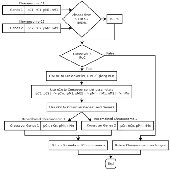
3.2.4.3 Crossover mechanisms . . . 97
3.2.4.4 Chromosome types . . . 97
3.2.4.5 Plug-in experiment code . . . 98
3.2.4.6 Using external software as (supplier of) objective functions . . . 98
3.2.4.7 Callable from external software . . . 99
3.2.4.8 Duplicate solutions control . . . 99
3.2.4.9 Constraints . . . 99
3.2.4.10 Chromosome Initialisers . . . 100
3.2.4.11 Population Initialisers . . . 101
3.2.4.12 Operator Configuration . . . 101
3.2.4.13 Problem-specific parameters . . . 102
3.2.4.14 Resume from previous run . . . 103
3.2.4.15 Command line run-time parameters . . . 105
3.2.4.16 Conclusion . . . 105
3.3 Benchmark test problems and results . . . 107
3.3.1 Problem definitions . . . 107
3.3.2 Benchmark test results . . . 109
3.4 Comparison with random search . . . 114
3.4.1 Random search algorithm . . . 115
3.4.2 Further optimisation test problems . . . 117
3.4.2.1 DTLZ1 . . . 117 3.4.2.2 DTLZ2 . . . 118 3.4.2.3 DTLZ3 . . . 118 3.4.2.4 DTLZ4 . . . 119 3.4.2.5 DTLZ5 . . . 119 3.4.2.6 DTLZ6 . . . 120 3.4.2.7 DTLZ7 . . . 120
3.4.2.8 DTLZ8 . . . 121 3.4.2.9 DTLZ9 . . . 122 3.4.2.10 MOKP 0/5 . . . 122 3.4.3 Results . . . 123 3.4.4 Summary . . . 130 3.5 Experiments in self-adaptation . . . 131 3.5.1 Summary . . . 132
3.6 Methods and materials . . . 134
4 A real-world airfoil application test case 137 4.1 Introduction to airfoil optimization . . . 137
4.2 Airfoil geometry . . . 138
4.3 Modifying XFoil . . . 140
4.4 Defining the optimisation . . . 141
4.5 Results . . . 144
4.5.1 Comparing algorithms . . . 144
4.5.2 Alternative crossover operator . . . 167
4.6 Airfoil comparison with other work . . . 171
4.6.1 Comparison summary . . . 178
4.7 Summary . . . 180
5 Multi-objective optimisation of an electrical power network 183 5.1 Electrical power networks . . . 183
5.2 Distributed generation . . . 185
5.3 Integrating with power market simulation . . . 189
5.4 Defining the optimisation . . . 190
5.4.1 Optimising for DG allocation by generation cost . . . 193
5.4.2 Optimising for DG allocation by sum of DG units . . . 195
5.4.3 Optimising for DG allocation by sum of DG units and line capacities . . . 198
5.5 Results . . . 200
5.5.1 Optimising for DG allocation by generation cost . . . 200
5.5.2 Optimising for DG allocation by sum of DG units . . . 210
5.5.3 Optimising for DG allocation and line capacities . . . 216
5.6 Comparison with random search . . . 227
5.7 Summary . . . 227
6 Conclusions and recommendations 231 6.1 Contributions . . . 231
6.2 Limitations . . . 232
6.3 Recommendations for further work . . . 233
6.3.1 Power optimisation . . . 233
6.3.2 Directed mutation . . . 234
6.3.3 Hybridise with a genetic program to act as a surrogate model235 6.4 Acknowledgements . . . 235
6.5 Concluding remarks . . . 236
A Poster 237 B Software information 239 B.1 Ganesh . . . 239
B.1.1 Ganesh Parameters . . . 239
B.2 Utility programs produced . . . 240
B.2.1 GADataCollect . . . 240
B.2.2 GAResultPlot . . . 241
B.2.3 GA-EvalFile . . . 242
B.2.4 PXmlTest . . . 243
B.2.5 Rastrigin’s function script . . . 243
C Tables for power optimisation 245
2.1 Euler diagram for P,N P, N P-complete, and N P-hard problems . . 36
2.2 solution spaces . . . 37
2.3 Global and local extrema . . . 38
2.4 Rastrigin’s function surface plot . . . 39
2.5 Rastrigin’s function contour plot . . . 40
2.6 General black box optimiser . . . 40
2.7 The effect of constraints . . . 42
2.8 Pareto front of a bi-objective problem . . . 43
2.9 Bi-objective optimisation Pareto front quadrants . . . 44
2.10 Pareto ranking example . . . 47
2.11 Nature-inspired metaheuristics . . . 55
2.12 EA sub-classes . . . 58
3.1 High level flow-chart of Ganesh . . . 81
3.2 Flow-chart of novel SAUBC operator. . . 91
3.3 Ganesh & Plugins UML . . . 93
3.4 UML for Plugins . . . 95
3.5 Benchmark test SCH . . . 110
3.6 Benchmark test FON . . . 110
3.7 Benchmark test POL . . . 111
3.8 Benchmark test KUR . . . 111
3.9 Benchmark test ZDT1 . . . 111 3.10 Benchmark test ZDT2 . . . 111 3.11 Benchmark test ZDT3 . . . 112 3.12 Benchmark test ZDT4 . . . 112 3.13 Benchmark test ZDT5 . . . 112 3.14 Benchmark test ZDT6 . . . 112
3.15 Benchmark test CONSTR . . . 113
3.16 Benchmark test BZDT2 . . . 113
4.1 NACA 0012 Airfoil . . . 139
4.2 Airfoil shown enclosed in free-form deformation hull . . . 139
4.3 Schematic diagram showing the interaction of Ganesh, FFD and XFoil. . . 139
4.4 An airfoil showing strengthening spars and vertical stiffeners. . . 142
4.5 Photograph of cross-section of aircraft wing . . . 142 13
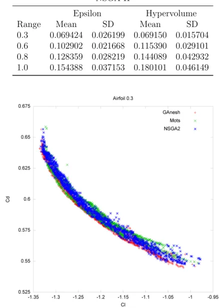
4.6 Diagram of Angle of Attack . . . 142 4.7 Results for range ±0.3. showing all samples of Ganesh, MOTS &
NSGA-II. . . 149 4.8 Results for range±0.3. showing all samples of Ganesh & MOTS only.150 4.9 Results for range ±0.6. showing all samples of Ganesh, MOTS &
NSGA-II. . . 150 4.10 Results for range ±0.8. showing all samples of Ganesh, MOTS &
NSGA-II. . . 151 4.11 Results for range ±1.0. showing all samples of Ganesh, MOTS &
NSGA-II. . . 151 4.12 Results for range ±1.0. showing Ganesh, MOTS & NSGA-II, and
GaneshG863 . . . 153 4.13 Results for range ±1.0. showing Ganesh, MOTS & NSGA-II, and
GaneshG863 with added airfoils. . . 154 4.14 Xfoil plot of an optimised airfoil ffd-2867 . . . 154 4.15 Xfoil plot of the unoptimised NACA 012 airfoil . . . 155 4.16 Trends of the means of the pM & ηM control parameters against
generation number for all ranges for all samples for Ganesh. . . 156 4.17 Trends of the means of the pC & ηC control parameters against
generation number for all ranges for all samples for Ganesh. . . 156 4.18 Trends of the standard deviations of pM &ηM control parameters
against generation number for all ranges for all samples for Ganesh. 156 4.19 Trends of the standard deviations of pC & ηC control parameters
against generation number for all ranges for all samples for Ganesh. 157 4.20 k-coords plot of Ganesh results for range ±1.0. at generation 863 . 159 4.21 k-coords plot of Ganesh results for range ±1.0. at generation 863
with selected airfoil . . . 160 4.22 k-coords plot showing Ganesh results for range±0.3, for all 20
sam-ples. samples . . . 160 4.23 k-coords plot showing normalised and scaled data from all samples
of all ranges of all algorithms . . . 162 4.24 k-coords plot showing normalised and scaled data from all samples
of all ranges of all algorithms with highlighted Ganesh range ±0.3 . 162 4.25 k-coords plot showing normalised and scaled data from all samples
of all ranges of all algorithms with highlighted Ganesh range ±1.0 . 163 4.26 k-coords plot as in Figure 4.25, but with MOTS data for all ranges
highlighted in green and superimposed . . . 164 4.27 k-coords plot as in Figure 4.26, with parameter 6 space covered by
Ganesh but not by MOTS . . . 164 4.28 k-coords plot as in Figure 4.27, with parameter 6 space covered by
NSGA-II but not Ganesh or MOTS . . . 165 4.29 k-coords plot zoom in of Figure 4.28 showing CDdetail . . . 165 4.30 k-coords plot for all samples of all ranges of all algorithms showing
best CD values . . . 167 4.31 State of the art airfoil performance . . . 174
4.32 Ganesh results for range ±1.0 at generation 863, atα = 15◦, Re=
2×10⁶ . . . 176
4.33 Xfoil plot of airfoil ffd-2268 at α = 3◦ . . . 177
4.34 Xfoil plot of airfoil ffd-3308 at α = 5◦, Re= 3×10⁵ . . . 177
4.35 Xfoil plot of airfoil ffd-3328 at α = 5◦, Re= 3×10⁵ . . . 178
4.36 Xfoil plot of airfoil ffd-3351 at α = 5◦, Re= 3×10⁵ . . . 178
5.1 Schematic diagram of a general large scale grid network . . . 185
5.2 A giant photovoltaic array, Nellis, Nevada USA. . . 186
5.3 Section of the American Electric Power System, Midwestern US, December 1961 . . . 187
5.4 IEEE 30-bus test system single line diagram . . . 188
5.5 Integration of Plexos with the self-adaptive MOOEA . . . 194
5.6 Integration of Plexos with the self-adaptive MOOEA . . . 196
5.7 Scatter plots for genCost/HC = 70 . . . 201
5.8 k-coords plot for genCost/HC = 70 . . . 202
5.9 Scatter plots for genCost/HC = 200 result . . . 203
5.10 & k-coords plots for genCost/HC = 200 result . . . 204
5.11 Scatter plots for gencost/HC = 35 . . . 205
5.12 Scatter & k-coords plots for gencost/HC = 35 . . . 206
5.13 k-coords plot of the entire data set for genCost/HC = 70 result . . 207
5.14 k-coords plot of the entire data set for genCost/HC = 70 result, best genCost . . . 208
5.15 k-coords plot of the data set for genCost/HC = 35 result . . . 209
5.16 k-coords plot for R008 in which V11 has 5 units, sumU,HC = 35 . . 212
5.17 k-coords plot for R003 in which V11 has 5 units, sumU,HC = 35 . . 213
5.18 Scatter plot for R008 showing sumU vs spotPrice, sumU,HC = 35 . 214 5.19 k-coords plot for R008 showing filtered results on V11, sumU,HC = 35215 5.20 k-coords plot of line capacities LC/sumU,HC = 35 . . . 221
5.21 k-coords plot of line capacities, LC,sumU,HC = 35 . . . 222
5.22 LC,sumU,HC = 35, final generation LC genes . . . 223
5.23 LC,sumU,HC = 35, best solutions’ LC genes . . . 224
5.24 LC,sumU,HC = 35, best solutions’ DG genes . . . 224
5.25 LC, HC = 35, varying line 6 capacity . . . 225
5.26 LC, HC = 35, varying line 22 capacity . . . 226
A.1 Poster for airfoil optimisation . . . 237
C.1 Node connections, ranked by number of connections per node, in node order. . . 253
2.1 Extended dominance relations to include approximation sets, from
the perspective of objective vectors . . . 46
2.2 Extended dominance relations to include approximation sets, from the perspective of approximation sets . . . 46
3.1 Benchmark test problems . . . 107
3.2 Mann-Whitney results for DTLZ1 comparison . . . 124
3.3 Means of ε- and hypervolume indicators for DTLZ1 test . . . 124
3.4 Mann-Whitney results for DTLZ2 comparison . . . 124
3.5 Means of ε- and hypervolume indicators for DTLZ2 test . . . 125
3.6 Mann-Whitney results for DTLZ3 comparison . . . 125
3.7 Means of ε- and hypervolume indicators for DTLZ3 test . . . 125
3.8 Mann-Whitney results for DTLZ4 comparison . . . 126
3.9 Means of ε- and hypervolume indicators for DTLZ4 test . . . 126
3.10 Mann-Whitney results for DTLZ5 comparison . . . 126
3.11 Means of ε- and hypervolume indicators for DTLZ5 test . . . 126
3.12 Mann-Whitney results for DTLZ6 comparison . . . 127
3.13 Means of ε- and hypervolume indicators for DTLZ6 test . . . 127
3.14 Mann-Whitney results for DTLZ7 comparison . . . 127
3.15 Means of ε- and hypervolume indicators for DTLZ7 test . . . 128
3.16 Mann-Whitney results for DTLZ8 comparison . . . 128
3.17 Means of ε- and hypervolume indicators for DTLZ8 test . . . 128
3.18 Mann-Whitney results for DTLZ9 comparison . . . 129
3.19 Means of ε- and hypervolume indicators for DTLZ9 test . . . 129
3.20 Mann-Whitney results for MOKP 0/5 comparison . . . 129
3.21 Means of ε- and hypervolume indicators for MOKP 0/5 test . . . . 129
3.22 Mann-Whitney results for self-adaptation vs non-self-adaptation comparison . . . 132
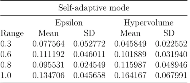
3.23 Means and standard deviations ofε- and hypervolume indicators of Ganesh in self-adaptive mode . . . 132
3.24 Means and standard deviations ofε- and hypervolume indicators of Ganesh in non-self-adaptive mode . . . 132
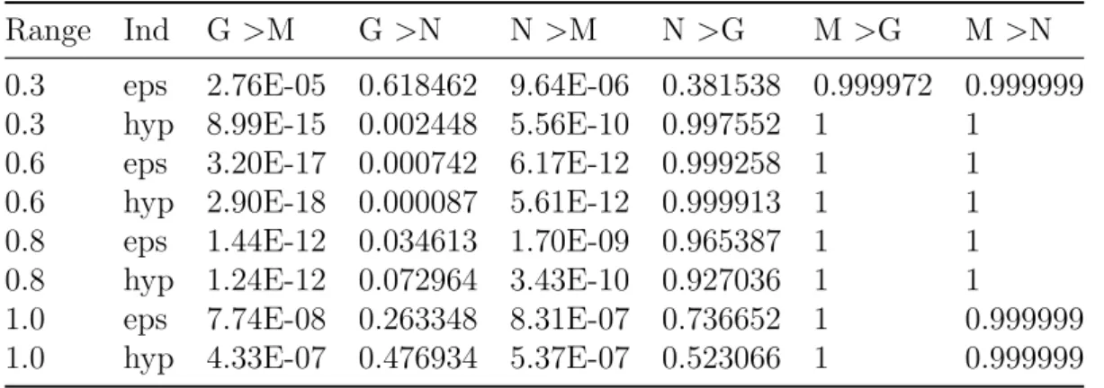
4.1 Kruskal-Wallis tests results for 3 independent data sets, comparing 20 sample runs per range for each of Ganesh (G), MOTS (M) & NSGA-II (N), showingp-values forα= 0.05. See also continuation table 4.2. . . 148 4.2 Continuation of table 4.1, for Ganesh, MOTS, & NSGA-II, giving
the interpretation of their relative performance. . . 148 4.3 Means of the ε- and hypervolume indicators provided by PISA for
Ganesh results. . . 148 4.4 Means of the ε- and hypervolume indicators provided by PISA for
MOTS results. . . 149 4.5 Means of the ε- and hypervolume indicators provided by PISA for
NSGA-II results. . . 149 4.6 Select airfoil design vectors from G863 of Ganesh for range ±1.0 . . 153 4.7 Mann-Whitney results for operator comparison . . . 169 4.10 Airfoil performance at α = 3◦. . . 175 4.11 Airfoil performance at α = 5◦. . . 175 4.12 Ganesh airfoil performance at α= 5◦ for Reynolds number 3×10⁵ . 176 4.13 Selected airfoils from G863 of Ganesh for range ±1.0 referenced in
this section. . . 176 5.1 The nodes (buses), their generator types, and associated variable
number in which the quantity of assigned DG units of that generator type is given. . . 193 5.2 New and previous best objective function results, from any solution,
optimising with OF1 = sumU . . . 210 C.1 Line limits of Plexos model . . . 245 C.2 The nodes and their total capacities determined by summing their
connected line capacities, in descending capacity order. The line capacity is counted at each node it is attached to, and the LowLimits have been rounded to the nearest integer. G,W & S are the DG unit types, heading their variables. . . 251 C.3 Node connections, ranked by number of connections per node, in
descending rank order, with DG variables. . . 252 C.4 OCGT fixed central generator characteristics. . . 255 C.5 Distributed Generation (DG) generator type characteristics . . . 255
ACO Ant Colony Optimisation. CD Coefficient of Drag.
CAD Computer-aided design. CAE Computer-aided Engineering. CFD Computational Fluid Dynamics. CL Coefficient of Lift.
CP Coefficient of Pressure.
DE Differential Evolution.
DG Distributed Generation or Generators; also describes the variables (gene alleles) that hold the number of units of generators of each type.
DoE Design of Experiments. EA Evolutionary Algorithm. EC Evolutionary Computing. EP Evolutionary Programming. ES Evolutionary Strategies. FE Function Evaluation. FEM Finite Element Methods. GA Genetic Algorithm. GUI Graphical User Interface. ISO Independent System Operator. JRE Java run-time environment. JVM Java Virtual Machine.
LC Line Capacities - The Maximum Flow ratings, in MW, of trans-mission lines; also describes the variables (gene alleles) that hold the values.
LMP Locational Marginal Pricing. MaOOP Many objective optimisation. MOO Multi-Objective Optimisation.
MOOEA Multi-Objective Optimising Evolutionary Algorithm. MOGA Multi-Objective Genetic Algorithm.
MOOP Multi-Objective Optimisation Problem. MOTS Multi-Objective Tabu Search.
NFL No Free Lunch - theorem. OCGT Open-Cycle Gas Turbine. OF Objective Function. OPF Optimal Power Flow.
PFapprox Approximate Pareto front - not the globally optimal front. PFopt Pareto-optimal front - the globally optimal front.
PSC Pseudo-code.
PSO Particle Swarm Optimisation. PT Polynomial Time.
PV Photovoltaic, of solar power generation. RDO Robust Design Optimisation.
SA Simulated Annealing.
SAMPSC Self-Adaptive Multi-point Swap Crossover. SAUBC Self-Adaptive Uniform Blend Crossover. SBX Simulated Binary Crossover.
Plugin A software component that adds a specific feature to an existing software application.
Speed of light c = 2.997 924 58×108 m−s (exact)
Elementary positive charge e = 1.602176565(35)×10−19 C (approx.)
P power MW (Js−1 x 10⁶) v voltage kV (V x 103) I current kA (A x 103)
to my mother, for the sacrifices she made for me
to my father, for the love of books
Introduction
This chapter is intended to address the following:
To describe the structure of the thesis.
To introduce the research of the thesis.
To provide the motivation for the research.
To highlight the novelties of the work.
1.1
Thesis organisation
The thesis is organised as set out below:
Chapter 1, here, sets out to describe the organisation of the thesis and to briefly introduce the work.
Chapter 2 provides a literature review of the subject areas encompassed in the research, considering the background and recent literature and identifying areas for the new research presented herein to be worthwhile and commensurate with the thesis objectives.
Chapter 3 sets out the value and description of the framework and multi-objective optimising evolutionary algorithm (MOOEA) produced in the course of this research, and reports on the benchmarks used and their outcomes.
Chapter 4 describes the optimisation of an airfoil using the framework and MOOEA of this work and an analysis and exploration of the results obtained.
Chapter 5 describes the optimisation of a model electrical power grid using the framework and MOOEA of this work, and analyses the results obtained.
Chapter 6 considers the work as a whole, describing its limitations, offering conclusions, and the possibilities of further work.
1.2
Background and motivation
Engineering design is a discipline that, through its applicability to so many areas (Rao, 1996) of our societies that are built upon technology, has a major impact upon contemporary living.
The increasing complexity of engineering designs, especially power and propul-sion systems, require the use of advanced computer modelling techniques to repre-sent such systems in an accessible manner, and the deployment of multi-dimensional analysis techniques to visualise their complex interdependencies in the most easily understandable manner.
Bloebaum and McGowan(2010) describe complex engineering systems as those systems in which the “. . . tightly coupled interacting phenomena yield a collective behavior [sic] that cannot be derived by the simple summation of the behavior [sic] of the parts”, where such systems tend to exhibit the following properties:
Have very many parameters defining the design
Have a challenging design space - constraints, discontinuities, non-linear
Challenge a priori preferences
Require trade-off compromises between goals of the system
The availability of relatively low cost computing hardware and software means that there is a greater possibility of improving engineering designs through the exploitation of optimisation in wider subject domains than in previous decades (Forresteret al.,2008). The targeting of multi-objective optimisation techniques at industrial engineering (Zalzala and Fleming,1997) has been shown to be tractable and successful and they have emerged, together with the techniques mentioned above, as key tools for establishing the appropriate degrees of complexity with which to replace previous simpler descriptions and solutions of designs and models. This is particularly true with regards to establishing design trade-offs, performing complex risk analysis, and ensuring the requisite variety to avoid and manage emerging tipping points.
Evolutionary computing (EC) techniques have been used to tackle a variety of non-linear (Nicolis, 1995) multi-objective optimisation problems successfully (Haupt and Haupt,2004, p. 174), and have been specifically applied to real-world complex engineering system optimisation problems (Gen and Cheng, 2000), but their success is governed by key parameters which have been shown to be sensitive to the nature of the particular problem, incorporating concerns such as the number of objectives and variables, and the size and topology of the search space, making it hard to determine the best settings in advance. The works of this thesis attempts to address this issue.
Improving electrical power grids, as an engineering design problem and as a matter of concern in many technological societies due to the relative fragility fo such networks, (Amin, 2003) taken together with the diminution of fossil fuel supplies and the need to cut pollution emissions, particularly of greenhouse gases, has become a matter of high research interest (Rylattet al.,2013). This work seeks to add an optimisation based-approach as a facilitator of design in the inception of (smart) power grids.
1.3
Thesis aims and objectives
This work therefore set out to create an evolutionary algorithm framework that is able to work on real-world engineering design problems, having the above char-acteristics, with the aim of being able to self-adapt in order to at least partially obviate the problem of determining the best parameter settings in advance. While work has been done in this area, commencing with Evolutionary Strategies (ES) by Schwefel and Genetic Algorithms (GA), as described byB¨ack (1992), this work creates both a novel framework advantageous to real-world situations, and an evo-lutionary algorithm (EA) with novelty in its self-adaptability, and certain other aspects, as detailed in Chapter 3. The EA is a multi-objective optimising EA (MOOEA) that is not limited by its construction in being able to work on any number of objective function dimensions, while the framework incorporates the MOOEA and provides means of applying it to new optimisation problems in a manner that enables the framework to be independent of the particular problem, as well as providing means of overriding certain default behaviours. However, al-though not architecturally limited in the number of objective functions (OFs) it can handle, in practice it has been found, as set out further in Chapter 2, that for a general EA, the more OFs are present, especially above three, the more likely the algorithm will find it hard to converge to an optimal set of solutions.
The framework of this research is then considered as a candidate for (smart) electrical power grid optimisation. Power networks can be improved in both tech-nical and economical terms by the inclusion of distributed generation which may include renewable energy sources. This work therefore sets out to propose and investigate a method to assist in the determination of the composition of optimal or high-performing power networks in terms of the type, number and location of the distributed generators, and to analyse the multi-dimensional results of the evolutionary computation component in order to reveal relationships between the network design vector elements and to identify possible further methods of im-proving models in future work.
In order to achieve the aims set out above, the evolutionary algorithm frame-work produced is benchmarked with standard tests from the literature (Zitzler
et al., 2000), to establish both correct functionality and its ability to converge with acceptable or better performance. A complex real-world engineering prob-lem is then to act as a further more exacting test of its capabilities, for which an airfoil optimisation case is used. The case chosen had been used in other studies of a similar nature, for which results of other algorithms were available to also act as benchmarks.
The airfoil optimisation case concerned the minimisation of drag and maximi-sation of lift coefficients of a well documented standard airfoil. The framework is integrated with a free-form deformation tool to manage the changes to the section geometry, and XFoil, a tool which evaluates the airfoil in terms of its aerody-namic efficiency. The performance of the framework/EA on this problem is com-pared with those of two other heuristic MOO algorithms known to perform well (Kipouros et al.,2012), the Multi-Objective Tabu Search (MOTS) and NSGA-II.
1.4
Publications
The following peer-reviewed papers were produced and published or accepted for publication in the course of this research:
1. A Self-adaptive Genetic Algorithm Applied to Multi-Objective Optimization of an Airfoil, (Oliver et al., 2013), presented by the author at the Evolve 2013 1 conference in Leiden, NL, published in the book of the proceedings. 2. An Evolutionary Computing-based Approach to Electrical Power Network
Configuration, (Oliver et al., June 2015), presented by the author at an ECCS’13 2 conference satellite workshop, in Barcelona; published in the journal Emergence: Complexity and Organization.
1EVOLVE - A Bridge between Probability, Set Oriented Numerics, and Evolutionary
Com-putation
3. Electrical Power Grid Network Optimisation by Evolutionary Computing, (Oliver et al., 2014), presented on the author’s behalf at the ICCS’14 3 conference in Cairns, AU, published in a special issue of the journalProcedia Computer Science.
4. Multi-Objective Optimization by Self-Adaptive Evolutionary Algorithm, (Oliver et al., expected 2016), an invited chapter in the book: EVOLVE - A Bridge between Probability, Set Oriented Numerics, and Evolutionary Computation 5, Series: Studies in Computational Intelligence, publication expected 2016.
1.5
Software Produced
There were two main software items produced in the course of this PhD, these being:
1. The self-adaptive multi-objective optimising evolutionary algorithm frame-work (named Ganesh, for brevity).
2. The set of plugins4 comprising the various optimisation problem definitions used in this work, which are available to be dynamically loaded and executed by Ganesh.
A number of utilities were also produced, to facilitate data manipulation and plotting, and these are detailed in Appendix B.
All these codes were produced with the intention that they be open source and are made available with an open-source licence, currently at: http://www. logiprime.com/ganesh/.
3The International Conference on Computational Science
4Although correctly spelled ‘plug-in’, it is commonly referred to as ‘plugin’ in technical
Heuristic multi-objective
optimisation algorithms
2.1
Introduction
This chapter provides a literature review of the general subject areas germane to this research, namely optimisation, heuristics, evolutionary computing, and related topics. In doing so, the context of the motivation for the aims of thesis are also made apparent.
Specific optimisation subject domains, namely airfoils and electrical power, are dealt with in those specific chapters.
2.2
Features of real-world optimisation
Optimisation is applicable to all areas of engineering which is inherently an area of real-world interaction, consequently engineers and researchers in all areas need to be aware of the possibilities in both theory and practice of optimisation (Rao,
1996). The engineering discipline sectors utilising optimisation include: structural,
thermal systems, chemical and metallurgical, electronics and electrical, mechani-cal, Aerodynamics, Combustion, propulsion, control, power and general engineer-ing design.
Rao (1996) notes that one way of classifying optimisation problems is by the nature of the decision vector elements, where static problems are those dependent upon some function of the decision vector, whereas dynamic problems are those in which each element of the design vector is a function of one or more other non-decision problem parameters. He gives the following characteristics in his assessment of real-world engineering design problems:
The design is in some way amenable to optimisation.
At least one of the objective functions of the optimisation is non-linear.
There are constraints that need to be adhered to.
At least some components of the design vector require real numbers.
The objective function outputs real numbers.
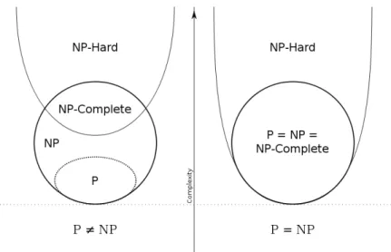
Gen and Cheng(2000) add that real-world complex engineering system prob-lems tend to be optimisation probprob-lems with complex constraints, and that such problems are often multi-dimensional in both decision space and objective space. Engineering may include unusual real-life matters that can be hard to model such as health and safety factors, aesthetics and other concerns, or may be com-putationally complex and could be classed as N P-complete, meaning they could be both in N P and N P-hard problem classes (Michalewicz et al.,1999).
Computational complexity (Garey and Johnson, 1979) is concerned with the inherent difficulty of problems, giving P as those decision problems1 that can be solved in polynomial time (PT) deterministically (by a deterministic Turing machine), which implies their time complexity function is given byO(p(n)) where pis some polynomial function andndenotes the size of the input. Problems not in
P are only solvable in exponential time, given byO(cn) (where c is some constant),
which means their solution time increases exponentially as n increases. P type problems may be solvable through deep insight, while those not inP require some
kind of exhaustive search approach. Problems not in P are considered intractable for other than smalln, with some exceptions; exceptions arise where the worst-case
does not occur generally, such as for the Simplex linear programming algorithm. The class of N P problems is then defined as those decision problems that can
be solved by PT nondeterministic algorithms2, which implies that their solution when = true is verifiable in deterministic PT. N P-hard problems are those ‘at
least as hard as the hardest problems in N P’, implying that they might not be solvable in PT. Figure 2.1 illustrates these set relationships, with the split between left and right being the unsolved question ‘P 6= N P?’ which essentially means whether every problem whose solution can be verified in PT can be solved in PT. If P 6= N P, then there are N P problems (such as the N P-complete ones) that might not be solvable in PT, but whose solution can be verified in PT.
A decision problem can be derived from an optimisation problem (Garey and Johnson,1979), whether it is maximising or minimising, by re-framing the problem as a bounded one and asking whether a solution exists within that bound B, for
example in the Travelling Salesman problem, is there a tour having length≤B, or in a maximisation, is there a solution with utility≥B. If the objective function can be evaluated ‘quickly’ (in PT at the most), then the decision problem is no harder than the original problem and can be possibly solved by a PT nondeterministic algorithm.
Thus real-world engineering problems often deal withN P-complete problems, and require algorithms with characteristics that give them a chance in tackling them pragmatically.
Figure 2.1: Euler diagram for P, N P, N P-complete, and N P-hard set of
problems, where left side shows P 6=N P and right sideP =N P.
2.3
Optimisation
2.3.1
Optimisation overview
Stated informally, optimisation is the process by which the minimum or maximum of a proposed function is found, and also the conditions, which means the values of the decision variables that the function takes as inputs, under which the result is obtained (Rao, 1996). The result of the function, which is termed the objective function (OF), thus represents the best outcome. When the optimisation seeks a minimum, the OF is often termed the cost function as one generally seeks to lower costs. Conversely, when seeking a maximum value, the OF is often termed the utility or fitness function, since these are naturally seen as ‘good’ and hence desirable.
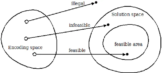
However, there are essential limitations imposed upon candidate solutions that may otherwise be considered optimal; a solution must be both feasible and legal
(Gen and Cheng,2000). A legal solution is one that can successfully be translated from the internal representation of the optimiser into the problem domain, whereas a feasible one is legal and resides in the feasible solution region of the domain, as in Figure 2.2. For example, a solution could represent a theoretically possible wing
and hence be legal, but not generate sufficient lift for it to be feasible in the real world.
Figure 2.2: Coding & solution spaces showing illegal and infeasible regions.
Without loss of generality, optimisation can be taken to be a minimisation, since by the principle of duality (Rao, 1996), a minimum can be transformed into a maximum, and vice-versa, by multiplying the result by −1, as the maximum of a function is equal to the minimum of the negative of that function. Henceforth unless specifically declared otherwise, minimisation will be assumed, as it indeed is in the internal mechanisms of the produced MOOEA (see Chapter 3).
A formal statement of optimisation can therefore be made as follows (B¨ack
et al., 1997):
~ x∈M f :M →R
f(~x)→min. (2.1)
in which~xis a vector of M parameters for the system, such that the objective
function f(~x) is minimised. To find the global optimum (2.1) it is necessary to:
find the vector~x∗
Optimisation problems occur in two broad classes: continuous and discrete, in which the former encompasses problems where M is infinite and M = Rn or where M is defined by equations and inequalities, and where the latter is defined
by M being in some way finite or in which points are isolated from each other, examples of which are combinatorial and integer problems (Bertsekas,1999).
Non-linear problems are of the continuous class, and can be thought of in two different ways, from a mathematics (a) or physics (b) viewpoint: (a) equations in which the unknowns are variables of a polynomial of degree two or more, or in the argument of a function which is not a polynomial of degree one; (b) The superposition principle does not hold, so have output not directly proportional to the input (Nicolis, 1995).
Having defined the process of global optimisation, in which the best solution from the entire search space is sought, it is then necessary to note that there may be regions within the solution space that have small values locally, the local
minima, that may deceive an optimiser into taking one of those as the global minimum, erroneously. Figure 2.3 illustrates.
Figure 2.3: Global and local minima and maxima
There is also the possibility that the objective function has two or more locally optimal solutions, in which case it is known as multimodal (Debet al.,1993). An
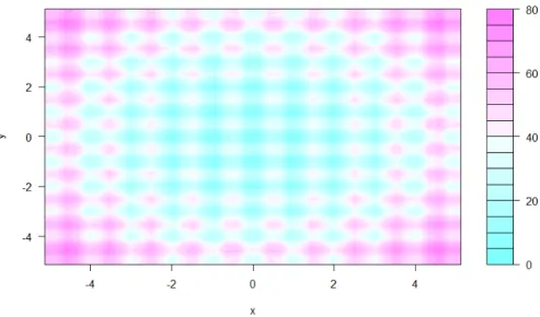
extreme example is given in Figure 2.4 which shows a surface plot from the R language of Rastrigin’s function in its 2D form (M¨uhlenbein et al.,1991), being a highly multimodal function having many local minima and maxima, and the global minimum (equation 2.3). Figure 2.5 shows a contour plot of the same function. Multimodal optimisation seeks to obtain a set of good solutions, comprising the best of the local optima along with, ideally, the global optimum if it can be found. When using methods which do not guarantee to find the global optimum, then it is more important to have a set to choose from since the global optimum may not be present and there may be different advantages and disadvantages between one local optimum and another.
Figure 2.4: Rastrigin’s 2D function as a surface plot, showing its many local
minima and maxima, where the global minimum is at (0,0) and equal to 0.
Rastrigin’s function in general form ofn dimensions
f(x) =An+ n X i=1 [x2i −Acos(2πxi)] (2.3) where A= 10 and xi ∈(−5.12,5.12) f(x) = 0 atx= 0
Figure 2.5: Rastrigin’s 2D function as a contour plot, showing the many minima and maxima as countour lines with colour indicating the amplitude.
In some optimisation problems the optimiser has no (or little) in-built ‘knowl-edge’ about the subject domain of the problem upon which it works, thus the optimiser acts as a black-box process (Schaefer and Nolle, 2006), transforming the input into an output (Figure 2.6). On these types of investigations, evolutionary computing is of particular relevance, and this is dealt with below in its own section.
Figure 2.6: A general black-box optimiser that finds the appropriate settings of x to yield the best value fory, in which x and y can take any form.
The “No free lunch” (NFL) investigation by Wolpert and Macready (1997) addresses the issue of choosing the best algorithm for a class of problems or even a particular problem, and whether such a choice is a priori possible. Their inves-tigation shows that not only is there no best algorithm, but that any algorithm that performs especially well on a particular problem class, will perform corre-spondingly worse than another on all other problem classes. This is true even for purely random search strategies. In particular, it is shown that if some knowl-edge of the problem can be incorporated, then performance tends to be better, although such knowledge is not always available. Uncertainty, in the form of lack of exact knowledge, about the precise objective function, f, can be expressed as a
probability distribution, P(f), and the performance of the optimiser then depends
on how well its strategies are aligned with P(f) (Wolpert,2012).
For example, in the electrical grid optimisation of Chapter 5, three of the ob-jective functions are effectively ‘black-box’, as they themselves depend on iterative procedures inside Plexos (commercial software that performs power calculations), about which the MOOEA has no information. The MOOEA can therefore not be stated to be a priori the best algorithm for this work; however it is not readily apparent that any other algorithm could substantiate that claim either. The fu-ture work described in Chapter 6, section 6.3.3 suggests a hybrid that could treat the GA as the originator of training examples for supervised learning by a genetic program (GP), with the goal of making the GA run in shorter overall times by using fast OFs produced by the GP.
Similarly, the airfoil optimisation of Chapter 4 is also effectively black-box, as it is the XFoil codes which perform the airfoil assessment for the MOOEA.
2.3.2
Multi-objective optimisation
So far this work has been concerned with the optimisation of a single quality criterion, a given problem’s objective function (OF), whereas in Chapter 1 it was noted that many real-world complex engineering systems tend to have more than one OF to be concerned about. This section therefore addresses the area of multi-criterion optimisation, which is more usually termed multi-objective optimisation (MOO), contemporarily.
Fonseca and Fleming(1998) made the point that optimisation constraints can also be taken as hard objectives, needing to be satisfied prior to the optimisation of the further, soft, objectives, and that on the other hand, problems having many objectives have in the past been transformed into single objective ones, with hard constraints, in order to solve them. Their proposed framework enabled constraints and OFs, both treated as functions, to be manipulated together. The effect of constraints can be visualised as in Figure 2.7.
Figure 2.7: Visualising the effect of constraints in a 2D objective space, Z
(Rao,1996).
However, the essence of MOO, is that there are two or moreconflicting objec-tive functions that need to be simultaneously optimised, such that each is satisfied. Systems having many OFs that are not competing, are not effectively MOO. An optimisation with OFs that are not in competition with each other, even where this has not been recognised, will naturally give rise to one solution to the problem, as is the case in single objective optimisation.
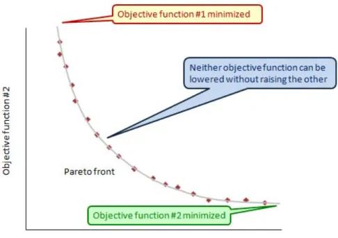
In problems that do have conflicting objectives, it naturally arises that there are a set of optimal solutions rather than just one, because no one solution can be better than all of the others with respect to all OFs, since to improve one OF necessarily degrades the other OFs (Deb, 1999). The global optimal set (in decision space) is known as the Pareto-optimal set, but other solution sets which approximate the global one, may be found and would be termed the local Pareto set or front. In objective space, the optimal set is known as the non-dominated
set, since each solution cannot be said to be dominated (be more optimal) by any other. Hence MOO requires trade-offs to be made, by some higher-level decision
maker (whether human or otherwise), in choosing a compromise solution to be the answer to the problem, as Figure 2.8 illustrates. Bearing in mind the Principle of Duality introduced at the start of 2.3, a two-dimensional (2D) MOO problem (MOOP), can be optimised in a number of ways, as Figure 2.9 illustrates, in which the direction of the convergence of the solutions are depicted depending upon the type of optimisation being performed.
Figure 2.8: The Pareto-optimal front of a bi-objective minimising optimisation
problem.
A corollary is that, unlike single objective optimisation, MOO gives rise to a new multi-dimensional space called the objective space, Z, in which the values of the OFs exist. There is then, a mapping between a given solution indecision space
and its corresponding point in theobjective space, noting that their vectors are of different dimensions, the former being ofn decision variables, and the latter of M
objective functions.
Moreover,Coelloet al.(2006) note, referencingB¨ack(1995), that for a general MOOP (and many particular ones), searching for the global optimum is an N P
-complete problem (Garey and Johnson,1979) for any system that is of more than minimal complexity, due to the exponential increase in the size of the search space,
Figure 2.9: Bi-objective optimisation Pareto front quadrants for OFsf1 &f2,
depending on the optimisaton of each OF being maximisation or minimisation (Deb,2013).
which depends upon the cardinality of both the decision vector and the permitted range of its components.
To formally define Multi-objective optimisation, the following can be stated, without loss of generality (Fonseca and Fleming,1998):
Minimise simultaneously n components fj, j = 1,· · ·, n of a function f of a
general decision variable x in a universeU, where:
f(x) = (f1(x),· · · , fn(x)) (2.4)
The Pareto dominance relation can then be defined as follows (assuming minimi-sation as above): A given vector u = (u1,· · · , un) is said to dominate another
vectorv = (v1,· · · , vn) if and only ifuis at least partly less thanv(up < v); stated
formally thus:
Pareto optimalityis then defined as: A solutionxu ∈ U is said to be Pareto-optimal
if and only if there is no xv ∈ U for which v = f(xv) = (v1,· · · , vn) dominates
u=f(xu) = (u1,· · · , un).
In practice, optimisation problems may be subject to restrictions on the values that one or more of their decision variables may take, or on the values held to be useful in the problem solution. Such constraints can usually take the form expressed as a function inequality: f(x) ≤ c, or f(x) < c, where c is a constant value and f is real-value function of x.
An inequality constraint function g(x) can manage a ≤0 constraint (or vice-versa) by multiplying both sides of the inequality by−1 or swapping one side of the inequality for the other (Deb,2012). For example, g(x)≤ybecomes−g(x)≥ −y, ory ≥g(x).
Equality constraints are harder to deal with, should be avoided if possible, and are a subject in their own right, especially in robust design optimisation (RDO), in which uncertainties are modelled to minimise their effects. Rangavajhala et al. (2007) examine approaches in RDO for equality constraint handling and provide a strategy, but here it is noted that if possible, relax an equality f(x) = c by replacing it with a combination of inequalities for special cases.
A constrained multi-objective optimisation problem, having functions (f1,· · · , fk), can thus be expressed without loss of generality as:
(fk+1(x),· · ·, fn(x))≤(gk+1,· · · , gn)
. . . in which x is a generic decision variable, in the universe U, and is subject to a positive number of constraints n −k applied component-wise (Fonseca and Fleming,1998). It is not necessarily true that a solution exists inU which satisfies such a constrained problem.
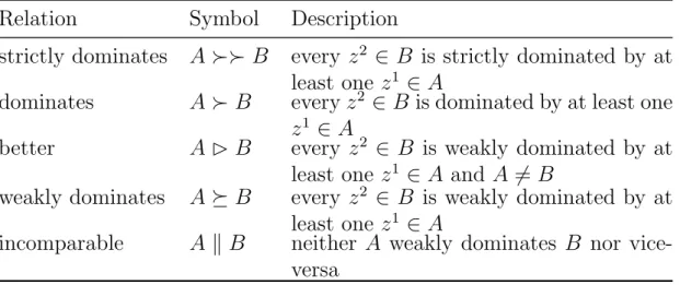
Zitzler et al. (2003) extended the definition of dominance by recognising that in practice, it is often very difficult to obtain the true global Pareto-optimal set,
whereas there may be one or more local Pareto sets, which they term approxi-mation sets, that may suffice to provide a choice of good enough solutions. The existence of two or more approximation sets motivates the definition for further dominance relations, as follows:
Approximation Set - LetA⊆ Z be a set of objective vectors for which A is an approximation set if any element of A does not dominate or is not equal to any
other vector in A, and for which the set of approximation sets is given by Ω. This enables all dominated solutions to be simply disregarded.
There then may exist the following dominance relations (Tables 2.1 and 2.2), considering objective vectors (solutions) z1 and z2, and approximation sets A & B:
Table 2.1: Extended dominance relations to include approximation sets, from
the perspective of objective vectors
Relation
Symbol
Description
strictly dominates
z
1z
2z
1is better than
z
2in all objectives
dominates
z
1z
2z
1is not worse than
z
2in all objectives
and better in at least one objective
weakly dominates
z
1z
2z
1is not worse than
z
2in all objectives
incomparable
z
1k
z
2neither
z
1weakly dominates
z
2nor
vice-versa
Table 2.2: Extended dominance relations to include approximation sets, from
the perspective of approximation sets
Relation
Symbol
Description
strictly dominates
A
B
every
z
2∈
B
is strictly dominated by at
least one
z
1∈
A
dominates
A
B
every
z
2∈
B
is dominated by at least one
z
1∈
A
better
A
B
B
every
z
2∈
B
is weakly dominated by at
least one
z
1∈
A
and
A
6
=
B
weakly dominates
A
B
every
z
2∈
B
is weakly dominated by at
least one
z
1∈
A
incomparable
A
k
B
neither
A
weakly dominates
B
nor
The Pareto dominance relation, defined in equation 2.5, can then be used to compare solutions within a population and rank them by how dominant and non-dominated they are with respect to the rest of the population (Fonseca and Fleming, 1993). Figure 2.10 shows an example ranking in which ‘level 1’ is the best performing set.
Figure 2.10: Pareto ranking example showing successive ranks
2.4
Performance of optimisation algorithms
The requirement to define what is meant by performance and to understand how algorithms perform arises from the desire to design algorithms and to gain insight into how well they work in practice, which in turn means how to measure their performance. Obtaining metrics for performance enables the comparison of algo-rithms, provides input into the design process, which may also include producing estimates of time and computational complexity and to assist in deciding how the algorithm should terminate.
Fundamentally, performance comprises both the quality of solutions produced and the effort (CPU time) or time (elapsed) required to elucidate them (Fonseca and Fleming, 1996). Effort is naturally a reflection of the time complexity of the algorithm running on the problem itself, usually expressed as ‘Big O’ notation, in which the time needed to run the algorithm is a function of the size of its input, where O(n) indicates a linear relationship (Garey and Johnson, 1979). Other
considerations include computational complexity (a measure of the theoretical difficulty of the problem), and resource usage such as memory, and possibly disk space.
The quality of the solutions achieved essentially means their objective function values in the final generation or iteration. If the global optima are known a priori
then the quality is relative to their closeness to them.
A necessary step in defining performance is to draw a distinction between the utility or cost function, more generally termed the objective function (OF), and the concept of fitness of solution. The optimisation problem is defined by the specification of the OF, whereas fitness is a measure of the desirability of a candidate solution at a given point in the execution of the algorithm. While the value of one may be equal to the value of the other in some single objective algorithms, the distinction is certainly necessary when considering algorithms in which the assessment of a given solution is dependent upon a vector of objective values (Fonseca and Fleming, 1997), and in MOOPs this is the case by definition. For MOOPs then, ‘performance’ encompasses a number of considerations, fore-most of which are those related directly to the Pareto optimal (PFopt) front which is the set of solutions which are globally optimal. Thus convergence to the PFopt front, both in terms of being able to achieve it and the rate of progress towards it, are basic concerns. The other primary concern is the diversity and spread of solutions along the PFopt front, or along the locally optimal approximation sets prior to convergence, since it is desirable, in the absence of knowledge about the possible solution set (that a domain expert might have), to obtain results from across the width of the (hyperplane of the) front (Fleming and Purshouse, 2001). The subsidiary concern of maintaining a degree of lateral diversity of solutions across objective space, in which solutions are perpendicular to the PFopt front, can be seen as a putative mechanism of performance improvement rather than as a direct measure of performance itself. Both cases of diversity are important in the performance of a GA as potentially good solutions should not be lost, where possible (Laumanns et al., 2001). Diversity of solutions helps prevent premature
convergence in the earlier stages of the process, and ameliorates the tendency to search in non productive directions later.
It is the case that the PFopt front may not be known, thus whether maximal convergence has been achieved is not always knowable, in which case performance in this regard can only be measured from an alternative known reference, such as an existing approximation front or a pre-defined set, typically of low quality points in objective space.
There are a variety of quantitative metrics for determining the spread or den-sity of solutions in objective space, which are required both for a quality measure of the algorithm final solution set (the wider and more even the spread, the better) but also to help the algorithm while running to assign a fitness to a solution, since it is usually the case that an algorithm wants to remove one or more solutions from a densely clustered location and allow more solutions at sparsely populated locations.
A density/crowding/sparsity metric may require finding the distance between two or more given solutions in objective space and there are a number of ways such a thing can be calculated, for example the distances of Manhattan, Eu-clidean, Chebyshev, Minkowski, among others. Normalisation of the objective function values may be necessary where OFs are scaled differently, in order that the distances computed for one dimension do not swamp those of another. These values may then be used to define a region in which other solutions are to be counted, or for example by summing for a given solution the distances of all other solutions to it (Deb et al., 2000). Diversity of solutions, however, comes at the price of increased computational expense (Deb et al., 2003). The fitness of a so-lution can then be derived as a function of both its quality and its proximity to other solutions, either through a sharing scheme (Fonseca and Fleming,1995a) in which fitness is degraded as a function of higher population density, or through the secondary application of density as a criterion when ranking would otherwise be the same.
Measures of convergence are calculated for the approximation front(s), in which diversity of solutions may be taken into account. Such metrics include:
Hypervolume (Zitzler and Thiele, 1998) was originally described as “the size of the space covered”, is a measure of how much space (area or hypervolume, depending on the dimensionality of the objective space), is dominated by an approximation front, thus it is not only an indicator of convergence but also of breadth of front.
(Unary) ε-indicator (Zitzleret al.,2003) is a measure of the minimum distance of translation needed to move every solution in the discovered front, so that the front weakly dominates the most converged front found, thus is an intu-itive measure of Pareto dominance.
R indicators Hansen and Jaszkiewicz(1998) are three different but related met-rics that provide an assessment of the difference between approximation fronts, but do not work in all cases. R1 estimates the number of times the solutions of one front are better than the other. R2 is a graded esti-mate of the superiority of one front over the other, and R3 indicates the proportion by which one front is better than the other. They require a set of utility functions together with assumed probabilities of their occurrence and a numerical integration technique to solve the integral. Deb and Jain(2002) suggest a weighted set of Tchebycheff metrics for the utility functions.
It is important to remember that each convergence metric is in some way deficient by itself in that they may not always be applicable, depending on the distribution of points in the approximation or reference fronts being compared, or may not provide all the information required. Where fronts are comparable, different metrics may indicate opposite conclusions, again depending on the nature of the fronts, for example a wide spread of solutions related to a front which is only partially better converged. Thus it is advisable to use more than one metric in such comparisons, with both qualitative (better) but also quantitative (better by how much) metrics being available (Zitzler et al., 2003). Zitzler et al. (2002)
showed that at least M metrics are needed to compare two or more fronts of an
M objective problem.
2.5
Heuristics and meta-heuristics
2.5.1
Heuristics
It has been noted above that MOOPs are often hard to solve as they tend not to be amenable to analytical methods due to their usual non-linearity and multi-dimensionality (both in decision and objective space), and also often or usually, having very large search spaces from which solutions must be picked. The sizes of the search spaces of such problems tends to preclude the use of exhaustive and complete searching, which would take too long to be practical, or even possible (since they may in theory take many years).
Moreover, multimodality tends to occur as soon as the number of OFs exceed one, for non-trivial competing objectives, even where each OF by itself is of single modality and is a convex function (Fonseca and Fleming, 1995b).
The inherent characteristics of these problems leads to the adoption of other methods which are determinedly less than complete explorers of the problem space, with the corollary that solutions found may not always be the best, but either the method returns the best solution often enough, or approximate solutions are deemed “good enough”.
Heuristics then, are “criteria, methods, or principles for deciding which among several alternative courses of action promises to be the most effective in order to achieve some goal.”, (Pearl, 1984). Heuristic methods require knowledge about the problem domain, and may be of a stochastic nature, but tend to have sim-ple, incomplete or unreliable information about the exact problem. There is an essential dichotomy at the heart of these methods: to be simple, yet effective. A common phrase used to describe them is “rule of thumb”, which in turn may
imply some sort of summation or scoring of elements or steps in the problem. The so-called Greedy heuristic (Atallah and Blanton, 2009) is a good example of such a method: it adopts the general strategy of adopting the locally optimal choice at each decision point with the hope that this will eventually find the global op-timum, while accepting that this will not always be the case; yet it needs specific knowledge about the problem in order to be used. The book of Polya(2004) is it-self a heuristic guide to solving problems generally, even though aimed specifically at mathematical problems.
The term meta-heuristic was introduced byGlover (1986) in his discussion of the Tabu search algorithm, which uses a heuristic, as above, but upon which is im-posed a further strategy - that of penalizing moves that take a path already taken, and an organised memory mechanism. Various metaheuristic implementations have found use in the real-world, tackling necessary tasks such as job scheduling and vehicle or network routing (S¨orensen and Glover,2013), in which any solution that works is “good enough” even if such may not be the global optimum.
It is frequently the case that in pursuing difficult problems, especially real-world engineering ones, that the Pareto-optimal set, PFopt, is neither known, nor indeed knowable analytically (Veldhuizen and Lamont, 2000), therefore until proven otherwise, it is usually necessary to assume that a given set of solutions obtained in a front, is an approximation to the global: PFapprox.
2.5.2
Meta-heuristics
The term metaheuristic is often found in the literature and as it is by nature inher-ently general, the definitions given for it tend to vary, nevertheless the following set of common properties are fundamental in describing it (Blum and Roli, 2003) :
Have a goal of exploring the search space efficiently to find (near) optimal solutions.
Use a variety of techniques from local searches to complex learning strategies.
Are often, or usually, non-deterministic, and approximate.
May possess mechanisms to avoid becoming trapped in local minima.
Are often described at a level of abstraction from a specific problem.
Are not problem-specific.
May be hybridised with some domain-specific knowledge as heuristics that are controlled by a higher level strategy.
May use organised memory to leverage search experience to determine the direction of the search.
A metaheuristic thus is both a framework and a set of concepts, strategies and mechanisms that are consistent, for the design of heuristic algorithms. S¨orensen and Glover (2013) refine the definitionmetaheuristic to be “a high-level problem-independent algorithmicframework that provides a set of guidelines or strategies to develop heuristic optimization algorithms”. They also note that problem-specific implementations of heuristic algorithms within a metaheuristic framework, are also metaheuristics.
Figure 2.11 depicts the broad categories of metaheuristcs that have been in-spired by nature, with the common thread that living organisms in some way necessitate optimisation in the struggle to survive long enough to reproduce, ex-cept for the simulated annealing (SA) algorithm (Kirkpatrick et al., 1983), which uses the metaphor of the annealing process of metallurgy, as a system having multiple potential energy states therefore being amenable to statistical mechanics (analysis of aggregate properties of atoms in solids or liquids).
Particle Swarm optimisation (PSO) introduced by Kennedy and Eberhart
(1995) is based on velocities of moving particles in 2, 3 or n-dimensional (hyper-)spaces, and acceleration towards solutions nearer to the global optima, where behaviour was inspired by flocking and foraging of birds and fish, but also the desire to model human social behaviour. However, there are similarities with evo-lutionary algorithms (EA), in that: it is stochastic; there is an operator (agent velocity adjustment) similar in effect to that of crossover in genetic algorithms (GA); the concept of fitness of a solution is used; and the group ‘knowledge’ of the best position found so far (gbest), being analogous to elitism. Each particle, termed agent, stores the coordinates of the best solution location it has visited (pbest) and tracks other agents in its vicinity, while maintaining a minimum sep-aration, that it is informed are the current local optima (lbest). At each step, the agent evaluates its fitness and is accelerated towardspbest andlbest positions, with weighted random adjustments to its acceleration vector. A significant difference to GAs is that a PSO agent only has access tolbest in other agents, whereas GAs swap chromosomes with many individuals. Another significant difference is that a PSO can be considered to be a “directed mutation” method, in that individu-als may be modified, related to their fitness, but no re-sampling occurs, unlike in evolutionary methods. Re-sampling is the creation of new solutions from existing ones; in canonical PSOs the population is fixed.
Ant colony optimization (ACO) (Dorigoet al.,1996), (Dorigo and Blum,2005) and its derivatives, share some common themes with PSO of animal behaviour and foraging, in which colonies of the same species attempt to maximise their net energy gain (food consumption versus the energy expended to acquire it) over time. In ACO, the agents are metaphorical ants that move stochastically over a landscape, communicating with each other by assigning values to the paths they have taken that are relative to their fitness (the metaphor has it that the fitness is indirectly proportional to the distance to the food and the path value is a pheromone trail, for example when used for the Travelling Salesman problem (TSP), shorter paths are travelled by more ants in a given time, thus acquire higher values). The path values are adjusted by the number of agents travelling