A Rule-based Method Applied to the Imbalanced Classification of
Radiation Toxicity
Juan L. Domínguez-Olmedo1, Jacinto Mata1, Victoria Pachón1 and Jose L. Lopez Guerra2 1Escuela Técnica Superior de Ingeniería, University of Huelva, Huelva, Spain
2Department of Radiation Oncology, University Hospital Virgen del Rocío, Sevilla, Spain
Keywords: Imbalanced Data Classification, Rules Discovery, Prostate Cancer.
Abstract: This paper describes a rule-based classifier (DEQAR-C), which is set up by the combination of selected rules after a two-phase process. In the first phase, the rules are generated and sorted for each class, and then a selection is performed to obtain a final list of rules. A real imbalanced dataset regarding the toxicity during and after radiation therapy for prostate cancer has been employed in a comparison with other predictive methods (rule-based, artificial neural networks, trees, Bayesian and logistic regression). DEQAR-C produced excellent results in an evaluation regarding several performance measures (accuracy, Matthews correlation coefficient, sensitivity, specificity, precision, recall and F-measure) and by using cross-validation. Therefore, it was employed to obtain a predictive model using the full data. The resultant model is easily interpretable, combining three rules with two variables, and suggesting conditions that are mostly confirmed by the medical literature.
1 INTRODUCTION
Prostate cancer (PC) is the most commonly diagnosed cancer affecting men, and the third leading cause of death in men in Europe (Ferlay et al., 2013). The American Cancer Society estimated that more than 200,000 men are diagnosed in the United States with 30,000 deaths (American Cancer Society, 2014). Although there is an improvement in tumor control rates using radiation dose escalation, PC radiotherapy is limited by the proximity of surrounding normal tissues and because of the observed dose-effect association with toxicity. It is essential to understand the true complications associated with doses delivered to normal anatomy, to ensure the delivery of a sufficient dose with minimal complications. The use of intensity-modulated and image-guided radiation therapy can decrease acute toxicity in PC patients (Valeriani et al., 2013); (Morimoto et al., 2014).
Within the field of artificial intelligence and, more specifically in machine learning, one of the methods employed to extract knowledge from data is the use of association rules. Association rule mining is a technique whose purpose is to extract strong and interesting relationships between patterns in a set of
data. An association rule takes the form A → C, where A (the antecedent) and C (the consequent) express a condition (or a conjunction of conditions) on variables of the dataset (Agrawal et al., 1993); (Rudin et al., 2013). The measures support and
confidence are used to assess the quality and importance of the association rules. The support measure evaluates the number of cases in which both the antecedent and the consequent of the rule hold. The confidence measure is the ratio between the support of the rule and the number of cases in which the antecedent holds. In order to filter the usual huge number of rules generated, the values
minsup (minimum support) and minconf (minimum confidence) are the thresholds that a rule has to satisfy to be considered of interest.
Subgroup discovery is a type of descriptive induction whose objective is to generate models based on rules using a predictive perspective. It emerged as the task of discovering properties of a population by obtaining simple (but significant) rules, using only one variable in the consequent: the class or target variable (Wrobel, 1997); (Gamberger et al., 2003); (Domínguez-Olmedo et al., 2015).
And also, numerous techniques have been proposed for classification problems. In this kind of
Domínguez-Olmedo, J., Mata, J., Pachón, V. and Lopez-Guerra, J.
A Rule-based Method Applied to the Imbalanced Classification of Radiation Toxicity.
task, a predictive model (classifier) tries to predict, with some certainty, the objective variable (of categorical type). Some examples of predictive methods are artificial neural networks, decision trees, logistic regression and Bayesian networks, among others (Hastie et al., 2009); (Golhar et al., 2017); (Cortés et al., 2015); (Liu et al., 1998). In binary classification tasks with imbalanced data, as in the case at hand, most algorithms are not usually capable of obtaining good results for the minority class and, therefore, the overall classification performance does not reach adequate values (Sun et al., 2009); (Rastgoo et al., 2016). The technique proposed in this paper has achieved an improved precision in both classes, thanks in part to an alternating selection of rules for each class.
The rest of the paper is organized as follows. Section 2 gives a description of the methods employed in this work. The experimental setup is presented in Section 3. Section 4 describes the experimental results and discussion. And the last section presents the conclusions.
2 METHODS EMPLOYED
2.1 Description of DEQAR-C
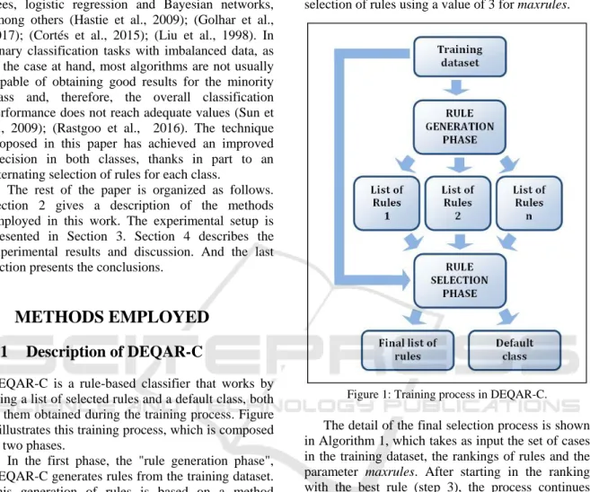
DEQAR-C is a rule-based classifier that works by using a list of selected rules and a default class, both of them obtained during the training process. Figure 1 illustrates this training process, which is composed of two phases.
In the first phase, the "rule generation phase", DEQAR-C generates rules from the training dataset. This generation of rules is based on a method developed to extract knowledge in the form of association rules (Domínguez-Olmedo et al., 2011); Olmedo et al., 2012); (Domínguez-Olmedo and Mata, 2016). It employs a deterministic approach to generate rules without a previous discretization of the numerical variables. Instead of discretizing, what may result in suboptimal results (Grosskreutz and Ruping, 2009), the process uses a dynamic generation of conditions. DEQAR-C obtains an ordered list of rules (called ranking) for each possible value of the class variable, storing separately the best rules in each class according to their values of confidence and support.
In the second phase, the "rule selection phase", a selection of the rules from all the rankings is done, by starting in the ranking of the rule with the highest confidence-support value and alternating iteratively between these rankings to select rules from them.
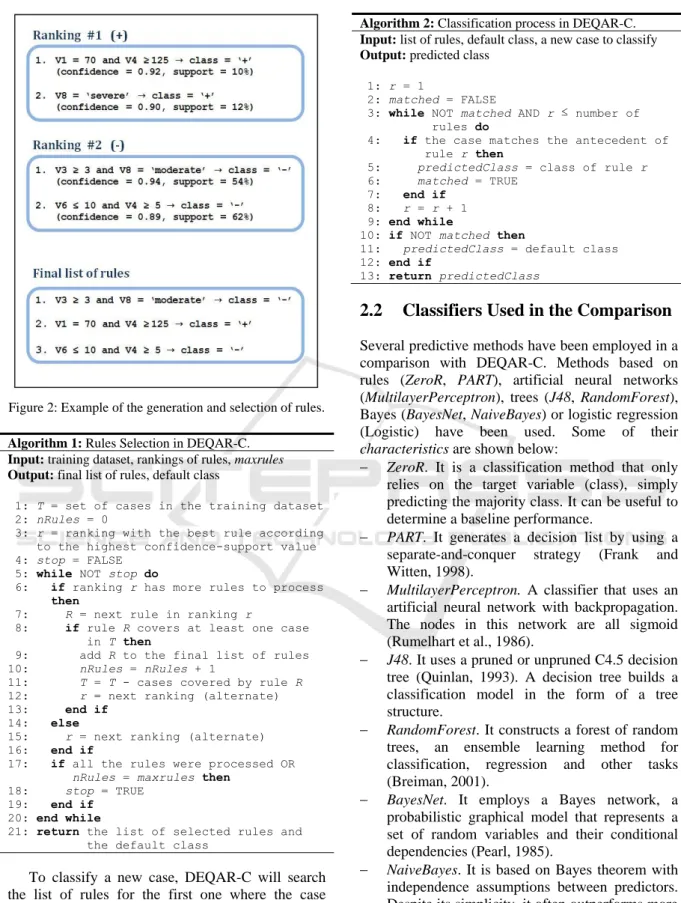
The parameter maxrules determines the maximum number of rules that will form the classifier. Figure 2 presents an example of this rule generation for a dataset with two classes, and also shows a possible selection of rules using a value of 3 for maxrules.
Figure 1: Training process in DEQAR-C.
The detail of the final selection process is shown in Algorithm 1, which takes as input the set of cases in the training dataset, the rankings of rules and the parameter maxrules. After starting in the ranking with the best rule (step 3), the process continues selecting rules from the different rankings, but only those rules covering some case not covered by a rule previously selected (step 8). In the case of a binary classification, the process would alternate in the selection of rules for the two possible classes (if there were still rules not processed in both rankings). The procedure stops when all the rules have been processed or the number of selected rules reaches
maxrules (step 17). At the end, the default class will be the one having the greatest number of cases not covered by any of the selected rules.
Figure 2: Example of the generation and selection of rules. Algorithm 1: Rules Selection in DEQAR-C.
Input: training dataset, rankings of rules, maxrules
Output: final list of rules, default class
1: T = set of cases in the training dataset 2: nRules = 0
3: r = ranking with the best rule according to the highest confidence-support value 4: stop = FALSE
5: while NOT stop do
6: if ranking r has more rules to process then
7: R = next rule in ranking r
8: if rule R covers at least one case in T then
9: add R to the final list of rules 10: nRules = nRules + 1
11: T = T - cases covered by rule R 12: r = next ranking (alternate) 13: end if
14: else
15: r = next ranking (alternate) 16: end if
17: if all the rules were processed OR nRules = maxrules then
18: stop = TRUE 19: end if
20: end while
21: return the list of selected rules and the default class
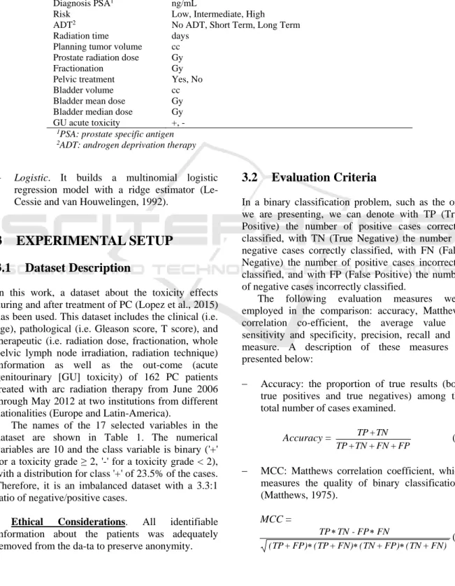
To classify a new case, DEQAR-C will search the list of rules for the first one where the case matches its antecedent, assigning the class of that rule. If no rule is found, the default class is assigned. Algorithm 2 shows this process.
Algorithm 2: Classification process in DEQAR-C. Input: list of rules, default class, a new case to classify Output: predicted class
1: r = 1
2: matched = FALSE
3: while NOT matched AND r ≤ number of rules do
4: if the case matches the antecedent of rule r then
5: predictedClass = class of rule r 6: matched = TRUE
7: end if 8: r = r + 1 9: end while
10: if NOT matched then
11: predictedClass = default class 12: end if
13: return predictedClass
2.2 Classifiers Used in the Comparison
Several predictive methods have been employed in a comparison with DEQAR-C. Methods based on rules (ZeroR, PART), artificial neural networks (MultilayerPerceptron), trees (J48, RandomForest), Bayes (BayesNet, NaiveBayes) or logistic regression (Logistic) have been used. Some of their
characteristics are shown below:
ZeroR. It is a classification method that only relies on the target variable (class), simply predicting the majority class. It can be useful to determine a baseline performance.
PART. It generates a decision list by using a separate-and-conquer strategy (Frank and Witten, 1998).
MultilayerPerceptron. A classifier that uses an artificial neural network with backpropagation. The nodes in this network are all sigmoid (Rumelhart et al., 1986).
J48. It uses a pruned or unpruned C4.5 decision tree (Quinlan, 1993). A decision tree builds a classification model in the form of a tree structure.
RandomForest. It constructs a forest of random trees, an ensemble learning method for classification, regression and other tasks (Breiman, 2001).
BayesNet. It employs a Bayes network, a probabilistic graphical model that represents a set of random variables and their conditional dependencies (Pearl, 1985).
NaiveBayes. It is based on Bayes theorem with independence assumptions between predictors. Despite its simplicity, it often outperforms more sophisticated classification methods (John and Langley, 1995).
Table 1: Variables and units of the dataset.
Variable Units/Values
Age years
Indication treatment Post-prostatectomy , Primary Prostate Cancer, Recurrence Radiation technique Tomotherapy, RapidArc
Gleason score 2..10
T stage T1 , T1b , T1c , T2 , T2a , T2b , T2c , T3 , T3a , T3b , T4 Diagnosis PSA1 ng/mL
Risk Low, Intermediate, High
ADT2 No ADT, Short Term, Long Term
Radiation time days Planning tumor volume cc Prostate radiation dose Gy
Fractionation Gy
Pelvic treatment Yes, No Bladder volume cc Bladder mean dose Gy Bladder median dose Gy GU acute toxicity +, -
1PSA: prostate specific antigen 2ADT: androgen deprivation therapy
Logistic. It builds a multinomial logistic regression model with a ridge estimator (Le-Cessie and van Houwelingen, 1992).
3 EXPERIMENTAL SETUP
3.1 Dataset Description
In this work, a dataset about the toxicity effects during and after treatment of PC (Lopez et al., 2015) has been used. This dataset includes the clinical (i.e. age), pathological (i.e. Gleason score, T score), and therapeutic (i.e. radiation dose, fractionation, whole pelvic lymph node irradiation, radiation technique) information as well as the out-come (acute genitourinary [GU] toxicity) of 162 PC patients treated with arc radiation therapy from June 2006 through May 2012 at two institutions from different nationalities (Europe and Latin-America).
The names of the 17 selected variables in the dataset are shown in Table 1. The numerical variables are 10 and the class variable is binary ('+' for a toxicity grade ≥ 2, '-' for a toxicity grade < 2), with a distribution for class '+' of 23.5% of the cases. Therefore, it is an imbalanced dataset with a 3.3:1 ratio of negative/positive cases.
Ethical Considerations. All identifiable information about the patients was adequately removed from the da-ta to preserve anonymity.
3.2 Evaluation Criteria
In a binary classification problem, such as the one we are presenting, we can denote with TP (True Positive) the number of positive cases correctly classified, with TN (True Negative) the number of negative cases correctly classified, with FN (False Negative) the number of positive cases incorrectly classified, and with FP (False Positive) the number of negative cases incorrectly classified.
The following evaluation measures were employed in the comparison: accuracy, Matthews correlation co-efficient, the average value of sensitivity and specificity, precision, recall and F-measure. A description of these measures is presented below:
Accuracy: the proportion of true results (both true positives and true negatives) among the total number of cases examined.
Accuracy = FP + FN + TN + TP TN + TP (1)
MCC: Matthews correlation coefficient, which measures the quality of binary classifications (Matthews, 1975). MCC = FN) + (TN FP) + (TN FN) + (TP FP) + (TP FN FP -TN TP (2)
Average value of sensitivity and specificity: sensitivity is the proportion of positives cases that are correctly identified as such, and specificity is the proportion of negatives cases that are correctly identified as such.
avg (Se, Sp) = 0.5 FP + TN TN FN + TP TP (3)
Precision: analogous to positive predictive value (PPV). precision = FP + TP TP (4)
Recall: analogous to sensitivity.
recall = FN + TP TP (5)
F-measure: the harmonic mean of precision and recall. F-measure = 2 ecall r precision ecall r precision (6)
4 EXPERIMENTAL RESULTS
4.1 Results of the Comparison
The classifiers previously mentioned were evaluated in the task about the prediction of toxicity effects in the radiotherapy treatment of PC. The evaluation measures were calculated by using stratified 10-fold cross-validation. Cross-validation reduces the variance of the estimates and improves the estimation of the generalization performance. In k-fold cross-validation, the original data is partitioned into k equal size subsets. Then, a single subset is retained as the validation data and the remaining k-1 subsets are used as training data. The process is repeated k times, with each of the k subsets used exactly once as the validation data (Arlot and Celisse, 2010). At the end, the final validation result is calculated from all the partial results.
The machine learning software Weka (Frank et al., 2016) was used to run the classifiers ZeroR,
PART, MultilayerPerceptron, J48, RandomForest,
BayesNet, NaiveBayes and Logistic. For a fair comparison, the final values of the parameters used in all the classifiers were the ones that yielded the best results after testing several combinations of values (grid search).
The results for accuracy, MCC and average value of sensitivity and specificity are displayed in
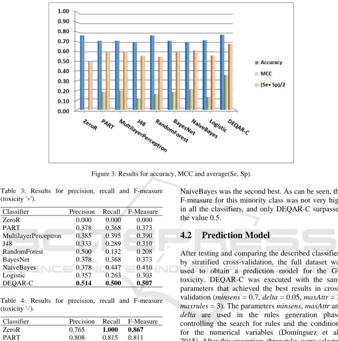
Table 2 and Figure 3. As can be seen, DEQAR-C obtained excellent results, which seems to support the proposed selection of high confidence-support rules for each class, not only to obtain high values of general accuracy but also to get a satisfactory prediction for both classes. The imbalance in the dataset (38 positive cases and 124 negative cases) adds more difficulty to the classification task. The results of DEQAR-C were the best regarding these three evaluation measures. The classifiers
NaiveBayes and MultilayerPerceptron also obtained good results, but the difference for MCC, in comparison with DEQAR-C, is important. Matthews correlation coefficient is generally regarded as being one of the best measures to describe the confusion matrix of true and false positives and negatives by a single number, especially suitable to the case of imbalanced data learning (Powers, 2011).
Table 2: Results for accuracy, MCC and average(Se, Sp). Classifier accuracy MCC avg(Se,Sp)
ZeroR 0.765 0.000 0.500 PART 0.710 0.185 0.592 MultilayerPerceptron 0.710 0.199 0.601 J48 0.698 0.118 0.556 RandomForest 0.765 0.161 0.546 BayesNet 0.710 0.185 0.592 NaiveBayes 0.698 0.210 0.611 Logistic 0.716 0.132 0.559 DEQAR-C 0.772 0.358 0.677
The results for the measures associated with a particular class (precision, recall and F-measure) are shown in Tables 3 and 4. DEQAR-C did not obtain the best F-measure result for negative toxicity (the majority class); but its result was close to the best, and obtained the best precision. Regarding the positive toxicity, DEQAR-C obtained the best precision, recall and F-measure; the classifier NaiveBayes was the second best. As can be seen, the F-measure for this minority class was not very high in all the classifiers, and only DEQAR-C surpassed the value 0.5.
Table 3: Results for precision, recall and F-measure (toxicity '+').
Classifier Precision Recall F-Measure
ZeroR 0.000 0.000 0.000 PART 0.378 0.368 0.373 MultilayerPerceptron 0.385 0.395 0.390 J48 0.333 0.289 0.310 RandomForest 0.500 0.132 0.208 BayesNet 0.378 0.368 0.373 NaiveBayes 0.378 0.447 0.410 Logistic 0.357 0.263 0.303 DEQAR-C 0.514 0.500 0.507
Figure 3: Results for accuracy, MCC and average(Se, Sp). Table 3: Results for precision, recall and F-measure
(toxicity '+').
Classifier Precision Recall F-Measure
ZeroR 0.000 0.000 0.000 PART 0.378 0.368 0.373 MultilayerPerceptron 0.385 0.395 0.390 J48 0.333 0.289 0.310 RandomForest 0.500 0.132 0.208 BayesNet 0.378 0.368 0.373 NaiveBayes 0.378 0.447 0.410 Logistic 0.357 0.263 0.303 DEQAR-C 0.514 0.500 0.507 Table 4: Results for precision, recall and F-measure (toxicity '-').
Classifier Precision Recall F-Measure ZeroR 0.765 1.000 0.867 PART 0.808 0.815 0.811 MultilayerPerceptron 0.813 0.806 0.810 J48 0.791 0.823 0.806 RandomForest 0.783 0.960 0.862 BayesNet 0.808 0.815 0.811 NaiveBayes 0.821 0.774 0.797 Logistic 0.791 0.855 0.822 DEQAR-C 0.848 0.855 0.851
The results for the measures associated with a particular class (precision, recall and F-measure) are shown in Tables 3 and 4. DEQAR-C did not obtain the best F-measure result for negative toxicity (the majority class); but its result was close to the best, and obtained the best precision. Regarding the positive toxicity, DEQAR-C obtained the best precision, recall and F-measure; the classifier
NaiveBayes was the second best. As can be seen, the F-measure for this minority class was not very high in all the classifiers, and only DEQAR-C surpassed the value 0.5.
4.2 Prediction Model
After testing and comparing the described classifiers by stratified cross-validation, the full dataset was used to obtain a prediction model for the GU toxicity. DEQAR-C was executed with the same parameters that achieved the best results in cross-validation (minsens = 0.7, delta = 0.05, maxAttr = 2,
maxrules = 3). The parameters minsens, maxAttr and
delta are used in the rules generation phase, controlling the search for rules and the conditions for the numerical variables (Domínguez et al., 2015). After this execution, three rules were selected (see Table 5) and the default class was set to '-'.
As can be seen, the rules are simple with two variables, because of the constraint due to the parameter maxAttr (maximum number of variables in the antecedent).
The combination of these three rules achieves a covering of 76% of the cases, and from the 39 remaining cases, 28 are negative ones.
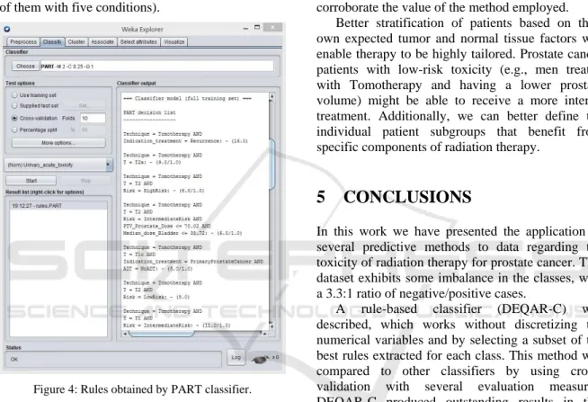
The simplicity of the obtained classifier also makes it more interpretable. It can be easily analyzed to discover the conditions most likely to be of influence in the toxicity effects, in contrast with the greater complexity of other models such as artificial neural networks or Random Forest. As an example, Figure 4 shows some of the 24 rules
Table 5: Rules obtained in the final classifier.
Antecedent GU acute toxicity
Technique = Tomotherapy AND Planning tumor volume ≤ 218.62 - Prostate radiation dose ≥ 70.02 AND Bladder volume ≥ 63.67 + Technique = Tomotherapy AND Fractionation ≤ 2.52 -
obtained after executing the classifier PART (some of them with five conditions).
Figure 4: Rules obtained by PART classifier.
4.3 Application to Clinical Practice
As can be seen by analyzing the rules in Table 5, five of the sixteen independent variables in the dataset are employed in the model: Technique,
Planning tumor volume, Prostate radiation dose,
Bladder volume and Fractionation. They can be considered of great relevance in this model for GU toxicity, because the predictions mainly depend on their values. Also, some relative importance could be established between them, because there exists an ordering in the rules and the search for a match follows this order.
These variables and their associated values could be seen as risk factors for GU toxicity. These risk factors are mostly confirmed by the literature (Acevedo-Henao et al., 2014); (Ahmed et al., 2013);
(Aizer et al., 2011); (Lopez et al., 2013), which may corroborate the value of the method employed.
Better stratification of patients based on their own expected tumor and normal tissue factors will enable therapy to be highly tailored. Prostate cancer patients with low-risk toxicity (e.g., men treated with Tomotherapy and having a lower prostate volume) might be able to receive a more intense treatment. Additionally, we can better define the individual patient subgroups that benefit from specific components of radiation therapy.
5 CONCLUSIONS
In this work we have presented the application of several predictive methods to data regarding the toxicity of radiation therapy for prostate cancer. This dataset exhibits some imbalance in the classes, with a 3.3:1 ratio of negative/positive cases.
A rule-based classifier (DEQAR-C) was described, which works without discretizing the numerical variables and by selecting a subset of the best rules extracted for each class. This method was compared to other classifiers by using cross-validation with several evaluation measures. DEQAR-C produced outstanding results in this classification task, with higher prediction performance in both classes than the rest of classifiers. Therefore, it was employed to obtain a predictive model using the full data. The simplicity of the model (three rules with two variables) also makes it more interpretable, which may be useful in obtaining knowledge from medical data and subsequently applying it into the clinical practice.
As future work, it would be interesting to test the proposed approach in another real classification problem or simultaneously with more datasets.
ACKNOWLEDGMENTS
The authors would like to thank Dr. Ignacio Azinovic for his support with the employed data.
The research presented in this paper was partially funded by the Regional Government of Andalusia (Junta de Andalucía) under grant number TIC-7629 and Spanish Ministry of Education and Science (Grant Number: TIN2009-14057-C03-03).
REFERENCES
Ferlay, J., Steliarova-Foucher, E., Lortet-Tieulent, J., Rosso, S., Coebergh, J.W.W., Comber, H., Forman, D. and Bray, F., 2013. Cancer incidence and mortality patterns in Europe: estimates for 40 countries in 2012.
European Journal of Cancer 49(6), 1374-1403. American Cancer Society, September 2014.
http://www.cancer.org/cancer/
prostatecancer/detailedguide/prostate-cancer-key-statistics.
Valeriani, M., Carnevale, A., Osti, M.F., de Sanctis, V., Agolli, L. and Enrici, R.M., 2013. Hypofractionated intensity-modulated simultaneous integrated boost and image-guided radiotherapy in the treatment of high-risk prostate cancer patients: a preliminary report on acute toxicity. Tumori 99(4), 474-479.
Morimoto, M., Yoshioka, Y., Konishi, K., Isohashi, F., Takahashi, Y., Ogata, T., Koizumi, M., Teshima, T., Bijl, H.P., van der Schaaf, A., Langendijk, J.A. and Ogawa, K., 2014. Comparison of acute and subacute genitourinary and gastrointestinal adverse events of radiotherapy for prostate cancer using intensity-modulated radiation therapy, three-dimensional conformal radiation therapy, permanent implant brachytherapy and high-dose-rate brachytherapy.
Tumori 100(3), 265-271.
Agrawal, R., Imielinski, T. and Swami, A., 1993. Mining Association Rules between Sets of Items in Large Databases. In Proceedings of ACM SIGMOD ICMD, 207-216.
Rudin, C., Letham, B. and Madigan, D., 2013. Learning theory analysis for association rules and sequential event prediction. Journal of Machine Learning Research, 14:3441-3492.
Wrobel, S., 1997. An algorithm for multi-relational discovery of subgroups. Principles of data mining and knowledge discovery, 78-87.
Gamberger, D., Lavrac, N. and Krstacic, G., 2003. Active Subgroup Mining: A Case Study in Coronary Heart Disease Risk Group Detection. Artificial Intelligence in Medicine 28, 27–57.
Domínguez-Olmedo, J. L., Mata, J. and Pachón, V., 2015. Deterministic Extraction of Compact Sets of Rules for Subgroup Discovery. In Proceedings of Intelligent Data Engineering and Automated Learning – IDEAL, 138-145.
Hastie, T., Tibshirani, R. and Friedman, J., 2009. The Elements of Statistical Learning: Data Mining, Inference, and Prediction. Springer-Verlag.
Golhar, M., Iwahori, Y., K. Bhuyan, M., Funahashi, K. and Kasugai, K., 2017. A Robust Method for Blood
Vessel Extraction in Endoscopic Images with SVM-based Scene Classification. In Proceedings of the 6th International Conference on Pattern Recognition Applications and Methods: ICPRAM, 148-156. Cortés, X., Serratosa, F. and Moreno-García, C., 2015. An
Interactive Model for Structural Pattern Recognition based on the Bayes Classifier. In Proceedings of the International Conference on Pattern Recognition Applications and Methods: ICPRAM, 240-247. Liu, B., Hsu, W. and Ma, Y., 1998. Integrating
classification and association rule mining. In
Proceedings of Fourth International Conference on Knowledge Discovery and Data Mining.
Sun, Y., Wong, A.K.C., Kamel, M.S., 2009. Classification of imbalanced data: a review. International Journal of Pattern Recognition and Artificial Intelligence 23(4), 687–719.
Rastgoo, M., Lemaitre, G., Massich, J., Morel, O., Marzani, F., Garcia, R. and Meriaudeau, F., 2016. Tackling the Problem of Data Imbalancing for Melanoma Classification . In Proceedings of the 9th International Joint Conference on Biomedical Engineering Systems and Technologies: BIOIMAGING (BIOSTEC).
Domínguez-Olmedo, J. L., Mata, J., Pachón, V. and Maña, M., 2011. A deterministic approach to association rule mining without attribute discretization. In Proceedings of the International Conference on Digital Information Processing and Communications, 188, 140–150. Domínguez-Olmedo, J. L., Mata, J., Pachón, V. and Maña,
M., 2012. Rule extraction from medical data without discretization of numerical attributes. In Proceedings of the International Conference on Health Informatics (HEALTHINF), 397-400.
Domínguez-Olmedo, J.L. and Mata, J., 2016. Comparison of Standard Discretization with a New Method for Quantitative Association Rules. IEEE Latin America Transactions 14(4), 1879-1885.
Grosskreutz, H. and Ruping, S., 2009. On Subgroup Discovery in Numerical Domains. Data Mining and Knowledge Discovery 19(2), 210–226.
Frank, E. and Witten, I. H., 1998. Generating Accurate Rule Sets without Global Optimization. In
Proceedings of the Fifteenth International Conference on Machine Learning, 144-151.
Rumelhart, D. E., Hinton, G. E. and Williams, R. J., 1986.
Parallel distributed processing: explorations in the microstructure of cognition. MIT Press Cambridge, 318-362.
Quinlan, R., 1993. C4.5: Programs for Machine Learning. Morgan Kaufmann Publishers, San Mateo.
Breiman, L., 2001. Random Forests. Machine Learning
45(1), 5-32.
Pearl, J., 1985. Bayesian Networks: A Model of Self-Activated Memory for Evidential Reasoning. UCLA Computer Science Department.
John, G. H. and Langley, P., 1995. Estimating Continuous Distributions in Bayesian Classifiers. In Proceedings of the Eleventh Conference on Uncertainty in Artificial Intelligence, 338-345.
Le-Cessie, S. and van Houwelingen, J. C., 1992. Ridge Estimators in Logistic Regression. Applied Statistics
41(1), 191-201.
Lopez Guerra, J. L., Matute R, Puebla F, Sánchez-Reyes A, Pontes B, Rubio C, Nepomuceno I, Acevedo C, Isa N, Lengua R, Praena-Fernandez JM, del Campo ER, Ortiz M. J and Azinovic I., 2015. Ethnic difference in risk of toxicity in prostate cancer patients treated with dynamic arc radiation therapy. Tumori 101(4), 461-8. Matthews, B. W., 1975. Comparison of the predicted and
observed secondary structure of T4 phage lysozyme.
Biochimica et Biophysica Acta (BBA)-Protein Structure 405(2), 442–451.
Arlot, S. and Celisse, A., 2010. A survey of cross-validation procedures for model selection. Statistics Surveys, 40-79.
Frank, E., Hall, M. A. and Witten, I. H., 2016. Data Mining: Practical Machine Learning Tools and Techniques. Morgan Kaufmann.
Powers, D. M. W., 2011. Evaluation: from precision, recall and F-measure to ROC, informedness, markedness and correlation. International Journal of Machine Learning Technology 2(1), 37-63.
Acevedo-Henao, C. M., Lopez, J. L., Matute, R. and Azinovic, I., 2014. Image-guided radiation therapy based on helical tomotherapy in prostate cancer: minimizing toxicity. Oncology Research and Treatment 37(6), 324-30.
Ahmed, A. A., Egleston, B., Alcantara, P., Li, L., Pollack, A., Horwitz, E.M. and Buyyounouski, M. K., 2013. A novel method for predicting late genitourinary toxicity after prostate radiation therapy and the need for age-based risk-adapted dose constraints.
International Journal of Radiation Oncology, Biology, Physics, 86(4), 709-15.
Aizer, A. A., Anderson, N. S., Oh, S. C., Yu, J. B., McKeon, A. M., Decker, R. H. and Peschel, R. E., 2011. The impact of pretreatment prostate volume on severe acute genitourinary toxicity in prostate cancer patients treated with intensity-modulated radiation therapy. International Journal of Radiation Oncology, Biology, Physics, 79(2), 379-84.
Lopez, J. L., Isa, N., Matute, R., Russo, M., Puebla, F. and Miran, K. M., 2013. Hypofractionated helical tomotherapy using 2.5-2.6 Gy daily fractions for localized prostate cancer. Clinical and Translational Oncology 15(4), 271-7.