Sequential imputation for models with latent
variables assuming latent ignorability
Lauren J Beesley, Jeremy M G Taylor, and Roderick J A Little
Department of Biostatistics, University of Michigan
Supplementary Materials
Contents
S1 Ignorability under a joint model (properties 1–5) 1
S2 Motivating the algorithm and performing parameter draws 3
S2.1 ImputingD(p). . . 4
S2.2 Imputing the latent variable . . . 5
S3 Bias of complete case analysis under LMAR 7 S4 Simulation study 9 S4.1 Simulation 1: linear mixed model with random intercept . . . 9
S4.2 Simulation 2: Cox proportional hazards mixture cure model . . . 12
S4.3 Simulation 3: mixture of normals . . . 15
S4.4 Simulation 4: Exploring identifiability and convergence . . . 17
S4.5 Simulation 5: Comparison of final analysis with and without imputedL . . . 19
S4.6 Simulation 6: more explorations for the CPH cure model . . . 21
S5 Example 1: identifiability for joint normal models 23 S5.1 Example 1.1: Measurement Error Model with Covariates . . . 23
S5.2 Example 1.2: linear mixed model example . . . 25
S6 Example 2: identifiability under LMAR for a mixture of GLMs 26 S6.1 Example 2.1: RY is Independent ofX (Nonidentifiable Model) . . . 26
S6.2 Example 2.2: RY Depends onX (Identifiable Model) . . . 27
S6.3 Simulation using nonidentifable model . . . 28
S6.4 Simulation using identifiable model . . . 29
S7 Implementation of the SMC imputation algorithm 31 S7.1 Drawing from a Distribution Known up to Proportionality . . . 31
S7.2 Linear mixed model with random intercept . . . 33
S7.3 Cox proportional hazards cure model algorithm . . . 37
S7.4 Mixture of GLMs . . . 40
S1
Ignorability under a joint model (properties 1–5)
Suppose that the data are directly modeled using a fully-specified joint model as follows:
f(D, L, R;ν) =
n
Y
i=1
f(Ri|Yi, Xi, Li;φ)f(Yi|Xi, Li;θ)f(Li|Xi;ω)f(Xi;ψ) (S1.1)
whereν= (φ, θ, ω, ψ) is the set of all model parameters. We assume a flat prior forνsuch
L(mis) ∼f(L(mis)|D, L(obs), R). This leads to draws from the joint posterior predictive
dis-tribution, f(D(mis), L(mis)|D(obs), L(obs), R) (Little and Rubin, 2002). Define ρ= (θ, ω, ψ).
We note the following properties of the (conditional) posterior predictive distributions:
Property 1: Under MAR and LMAR, we can ignore R = (RD, RL) when imputing
D.
The missingness mechanism is ignorable for imputingD(mis)iff(D(mis)|D(obs), L, R) =
f(D(mis)|D(obs), L). Using assumptions (1) and (2) and assuming φ and ρ are distinct,
f(D(mis)|D(obs), L, R) = 1 f(D(obs), L, R) Z Z f(D, L, R, ν)dρdφ = 1 f(D(obs), L, R) Z f(R|D, L;φ) Z f(D, L;ρ)f(ρ)dρ f(φ)dφ =f(D
(mis)|D(obs), L)f(D(obs), L)
f(D(obs), L, R)
Z
f(R|D(obs), L;φ)f(φ)dφ
=f(D(mis)|D(obs), L)
Therefore, the missingness mechanism is ignorable for imputing D. A similar result for
a related latent ignorable missingness setting was shown in Harel (2003). We note that in practice, draws from the posterior predictive distribution are obtained by first
draw-ing the model parameter ρ from its posterior distribution and then drawing D(mis) from
f(D(mis)|D(obs), L, R;ρ). We can perform both of these draws ignoring R.
Property 2: Under MAR (but not under LMAR), we can ignore R = (RD, RL) when
imputing L.
The missingness mechanism is ignorable for imputingL(mis)if f(L(mis)|L(obs), D, R) =
f(L(mis)|L(obs), D). Again using assumptions (1) and (2) and assuming φ and ρ are
dis-tinct, f(L(mis)|L(obs), D, R) = 1 f(L(obs), D, R) Z Z f(D, L, R, ν)dρdφ = 1 f(L(obs), D, R) Z f(R|D, L;φ) Z f(D, L;ρ)f(ρ) dρf(φ)dφ =f(L
(mis)|L(obs), D)f(L(obs), D)
f(L(obs), D, R)
Z
f(R|D(obs), L;φ)f(φ)dφ
Suppose first that missingness is MAR. Then, f(R|D(obs), L;φ) = f(R|D(obs), L(obs);φ)
and f(L(mis)|L(obs), D, R) = f(L(mis)|L(obs), D). Therefore,R is ignorable. Under LMAR,
however, the termR f(R|D(obs), L;φ)f(φ)dφdepends on L(mis), so R is not ignorable.
Property 3: Suppose that missingness in subset S of {D, L} is MAR. We can ignore the corresponding subset of R when imputing L provided a distinctness property holds.
Let RS denote the set of missingness indicators for S and R−S denote the
missing-ness indicators for the remaining variables in{D, L}. Note by assumption (2),L⊂S. Let
f(R−i S|Di, Li;φ) =f(R−i S|D (obs) i , Li;φ−S) andf(RSi|Di, Li, R−i S;φ) =f(RSi|D (obs) i , L (obs) i ;φS).
Assume also that φ−S and φS are distinct (a priori independent). Then we have
f(R|D(obs), L;φ) =f(RS|D(obs), L(obs);φS)f(R−S|D(obs), L;φ−S) =⇒
f(L(mis)|L(obs), D, R)∝f(L(mis)|L(obs), D)
Z
The contribution ofRS drops out of the posterior predictive distribution, so RS is
ignor-able. A similar result, called “ignorability for submodels”, was shown in Harel (2003).
For an example of submodel ignorability, see our data application in Section 6.
Property 4: R is ignorable for ρ in a final analysis using only imputed D under MAR
Suppose we perform our final analysis using the imputed values ofD but ignoring the
imputed L and again suppose that φ andρ are distinct. In a Bayesian analysis, we want
to make inference from the joint posterior ofφ and ρ:
f(ν|D, L(obs), R)∝f(R|L(obs), D;ν)f(L(obs), D;ρ)f(ν)
∝
Z
f(R|L, D;φ)f(L(mis)|L(obs), D;ρ)dL(mis)
f(L(obs), D;ρ)f(φ)f(ρ)
∝f(R|L(obs), D(obs;φ)f(φ)f(L(obs), D;ρ)f(ρ) under MAR
The posterior distributions of φ andρ separate, and the posterior forρis independent of
R. Therefore, we can ignoreR for inference aboutρ under MAR.
Property 5: A final analysis for making inference about ρ using imputed D (but not imputed L) and ignoring R is valid but not fully efficient under LMAR.
Under the setting of Property 4 except assuming LMAR, we again have that
f(ν|D, L(obs), R)∝
Z
f(R|L, D;φ)f(L(mis)|L(obs), D;ρ)dL(mis)
f(φ)f(L(obs), D;ρ)f(ρ)
Under LMAR, f(R|L, D;φ) depends on L(mis), so the contribution of R and φ does not
factor out of the integral. Therefore, we cannot separate φ and ρ in the above
equa-tion. We rewrite the above equation as f(ν|D, L(obs), R) ∝ h(ν)f(ρ|D, L(obs)) where
h(ν) = R f(R|L, D;φ)f(L(mis)|L(obs), D;ρ)dL(mis)f(φ). Clearly, ν and ρ are not
dis-tinct. However, L is MAR given imputed D. Under the ignorability conditions in
Lit-tle and Rubin (2002) (pg. 119–120), inference ignoring the contribution of R (using
f(ρ|D, L(obs))) will be valid from a frequency perspective but may not be fully efficient.
Intuitively, the loss of efficiency comes from a loss of information about the missing L
that comes from ignoring R under LMAR. However, analysis is still valid since missing
L is MAR givenD.
S2
Motivating the algorithm and performing
param-eter draws
In this appendix, we provide more details regarding the univariate imputation steps for
imputing missing values inDandL. In particular, we discuss distributions we can use to
perform the parameter draws within the sequential imputation algorithm. Our proposed method for drawing model parameters within a given univariate imputation step will
de-pend on whether we are performing imputation of the latent variable or a variable in D.
Here, we will suppose that Lis imputed from the kernel in (2) from the main paper and
that missing X and Y are imputed from working imputation models that may or may
not correspond (3) and (4) from the main paper. Therefore, the following exploration can be applied when outcomes and covariates are imputed using (3) and (4) or using
joint distribution,f(D, L, R;ν). We partitionν = (φ, ρ) where φ represents the
missing-ness model parameters and ρ represents all other model parameters. We assume that ρ
and φ are distinct (a priori independent). Suppose that we specify ˜f(D(ip)|D(i−p), Li; ˜ρp)
to be the working conditional distribution of D(ip) used for imputation. We can view
˜
f(D(ip)|Di(−p), Li; ˜ρp) as an approximation of f(D
(p)
i |D
(−p)
i , Li;ρ). If we use the form of
the full conditional distribution as in (3) and (4), ˜ρp will be a subset of ρ. If we impute
using regression models, ˜ρp may not be directly related toρ. We suppose that we impute
L fromf(Li|Di, Ri;ν) as described in (2).
S2.1
Imputing
D
(p)InSection S1, we show how, when missingness is LMAR, we can imputeD(mis)ignoring
the contribution ofR (assuming some distinctness properties). This is a result of the
as-sumption that missingness is conditionally independent of D(mis). Rather than imputing
D(mis) directly fromf(D(mis)|D(obs), L), we instead obtain a draw of D(mis) by iteratively
drawing missing values of each D(p,mis) from f(D(p,mis)|D(p,obs), D(−p), L) or from an
ap-proximated version, ˜f(D(p,mis)|D(p,obs), D(−p), L), treating the most recent imputations for
the other variables as if they were observed data (including L).
At a given iteration, we want to draw missing values of D(p) under MAR and LMAR
from its posterior predictive distribution: ˜
f(D(p,mis)|D(p,obs), D(−p), L) = Z
˜
f(D(p,mis)|D(p,obs), D(−p), L; ˜ρp) ˜f( ˜ρp|D(p,obs), D(−p), L)dρ˜p
This integral suggests an approach for drawing from the posterior predictive distribution.
Assuming that the data Di(p) across subjects iare conditionally independent givenL and
D(i−p), we can obtain a draw from the posterior predictive distribution by performing the
following (Little and Rubin, 2002):
1) Draw ˜ρp from ˜f( ˜ρp|D(p,obs), D(−p), L)
2) Draw missing D(ip) from ˜f(D(ip,mis)|Di(p,obs), Di(−p), Li; ˜ρp) = ˜f(D
(p)
i |D
(−p)
i , Li; ˜ρp).
We note that step 1) involves drawing ˜ρp conditioning on D(p,obs) using only the
observed part of D(p). This is consistent with chained equations imputation in which we
draw parameter values using only the observed values of D(p) (Van Buuren et al., 2006).
The step for drawing ˜ρp conditioning only on the observed data can be accomplished
by using the data with observed values for D(p) and prior ˜f( ˜ρp). If we assume the prior
distribution is proportional to 1, we can draw ˜ρp by fitting model ˜f(D(p)|D(−p), L; ˜ρp) to a
bootstrap sample of the data with observed values forD(p). We note that while this step
for drawing ˜ρp does not use the most recent imputation of D(p), it does use the imputed
values for L.
An alternative to the above is to draw ˜ρp using a Gibbs-type approach. In Gibbs
sampling-type imputation algorithms, parameter values are drawn using all of the most
recent imputed data, including imputed values forD(p) from the previous iteration. This
approach is also used in SMC-FCS, a modified chained equations approach proposed in Bartlett et al. (2014). If preferred, we can obtain valid parameter draws using this approach as well. We note that we can write
˜
f( ˜ρp|D(p,obs), D(−p), L) =
Z ˜
f( ˜ρp|D(p), D(−p), L) ˜f(D(p,mis)|D(p,obs), D(−p), L)dD(p,mis)
The above integral suggests that we can obtain a draw from ˜f( ˜ρp|D(p,obs), D(−p), L) by
iteration, which was drawn from ˜f(D(p,mis)|D(p,obs), D(−p), L). Rather than drawing pa-rameter values using the complete case data as is in the usual implementation of chained equations, we can alternatively draw parameters conditioning on the imputed values of
D(p) from the last iteration. We use this approach for drawing parameters in our
simu-lations and in our presentation of the proposed method in the main paper.
Rather than approximating the distributions for each variable with missingness with a regression model for imputation, suppose that we impute all variables using the kernel
forms in (2), (3) and (4). In this case, ˜ρpis is a subset ofρ. For simplicity, we might choose
to perform only a single set of parameter draws per iteration of the sequential imputation algorithm and use that set of parameter draws for imputing all of the variables in that iteration. This approach is used in Gibbs sampling-type algorithms. In this case, we
might perform a set of parameter draws for ρ in the step for imputingL, which involved
drawingρusing methods treatingLas latent as described in the following section. Then,
we can use that same drawn value for ρ for imputing the covariate/outcome values. We
note that the above derivations above suggest that we should drawρ conditioning on the
imputed values of Lwhen we are imputing covariates/outcomes. In our experience,
how-ever, a single draw of ρ using the above approach generally produces good results when
we perform our final analysis using only the imputed values ofD. When we perform our
final analysis using the imputed values of D and L, drawing ρ before each imputation
can sometimes produce improved parameter coverage.
S2.2
Imputing the latent variable
In the imputation step for L at a given iteration of the sequential algorithm, we aim to
draw missing values from the posterior predictive distribution:
f(L(mis)|L(obs), D, R) =
Z
f(L(mis)|L(obs), D, R;ν)f(ν|L(obs), D, R)dν
under LMAR and the posterior predictive distribution:
f(L(mis)|L(obs), D) =
Z
f(L(mis)|L(obs), D;ρ)f(ρ|L(obs), D)dρ
under MAR. Here, we treat the most recent imputations for D as if they were the
ob-served data. As before, this integral suggests an approach for drawing from the posterior predictive distribution. We can obtain a draw of the posterior predictive distribution by performing the following:
1) Under LMAR, draw ν fromf(ν|L(obs), D, R).
Under MAR, draw ρ fromf(ρ|L(obs), D).
2) Under LMAR, draw missing Li from f(L
(mis)
i |L
(obs)
i , Di, Ri;ν) =f(Li|Di, Ri;ν).
Under MAR, draw missing Li from f(L(imis)|L
(obs)
i , Di;ρ) =f(Li|Di;ρ)
We note here that we are assuming that Li values are conditionally independent across
different values of i. Suppose our outcome model is a linear mixed model with a random
intercept,L. Thenihere would index the clusters (rather than the units within clusters),
and a single value of L would be drawn for all units within the cluster.
Drawing
ρ
under MAR
Drawing
ρ
and
φ
under LMAR
We note that
f(ν|L(obs), D, R) = f(ρ|L(obs), D, R, φ)f(φ|L(obs), D, R) (S2.2)
WhenLis partially latent (so it is partially observed), we can draw values ofνusing only
the subjects withL observed. When Lis fully latent, however, drawing from (S2.2) may
not be so simple. Therefore, we will propose an alternative approach that can be applied
for latent and partially latent L. We will consider how to draw φ and ρseparately using
the factorization in (S2.2).
We first consider how to draw values for ρ fromf(ρ|L(obs), D, R, φ). We have that
f(ρ|L(obs), D, R, φ)∝f(L(obs), D, R;ρ, φ)f(ρ)
∝f(R|D, L(obs);ν)f(L(obs), D;ρ)f(ρ)
This kernel separates into two factors: one that depends on φ and R and one that does
not. We note that L is treated as MCAR when L is fully latent and is assumed to be
MAR whenL is partially latent, so the missingness inL is ignorable given D(obs). When
we condition on the imputed D, we can make valid inference about ρ (in a frequentist
sense) without conditioning on R and φ (Little and Rubin, 2002). However, R does
contain some information about the value of L under LMAR (ν and ρ are clearly not
distinct) and therefore would contribute some information about ρ. Ignoring R when
drawing ρ, therefore, may result in a loss of efficiency. We can validly (but with some
potential loss of efficiency) ignore the contribution of R and φ tof(ρ|L(obs), D, R, φ) and
instead drawρ fromf(ρ|L(obs), D). This is important because it may be difficult to draw
from f(ρ|L(obs), D, R, φ), but a draw from f(ρ|L(obs), D) can be obtained using standard
methods that treat L as latent or partially latent and ignoringR.
We now consider how to draw values forφ. The distributionf(φ|L(obs), D, R) may be
difficult to draw from under LMAR assumptions since this distribution does not condition
onL(mis). We instead use the integral decomposition:
f(φ|L(obs), D, R) =
Z
f(φ|L, D, R)f(L(mis)|L(obs), D, R)dL(mis)
We can obtain a valid draw fromf(φ|L(obs), D, R) by instead drawing fromf(φ|L, D, R)
using the most recent imputation of L, which was drawn from f(L(mis)|L(obs), D, R).
Therefore, we can draw values of φ directly using the most recent imputed values of L.
This is easier than drawing fromf(φ|L(obs), D, R) because it can directly incorporate the
working LMAR model for the missingness mechanism without integrating out missing
values of L. We do not choose to use this same integral decomposition approach for
drawingρ as our proposed approach (which does not condition on the most recent
impu-tation of L) tends to result in more stable convergence properties in our experience (for
S3
Bias of complete case analysis under LMAR
In the main paper, we claim that we may expect bias in complete case analysis when
missingness in a covariate or outcome depends on the latent variable,L. Here, we provide
some justification for this claim, which may initially seem unintuitive. In usual regression analysis, complete case analysis is valid (but not fully efficient) when missingness in the
covariates/outcome does not depend on the outcome value conditional on X. However,
missingness can depend on other missing covariate values. The same does not apply when
missingness in covariates or the outcome depend on latent L.
Let’s consider the simple setting in which Y andX are univariate. Suppose first that
L was fully observed, so covariate and outcome missingness is then missing at random.
The two models of interest are f(L|X) and f(Y|X, L). If L is fully observed, we do
not expect bias in estimating parameters related tof(Y|X, L) unless sampling is directly
related to Y. However, we may run into bias in estimating parameters related f(L|X).
Suppose f(L|X) is a logistic regression model as it is in the Cox proportional hazards
mixture cure model. In this case, if missingness only depends on L, then would not
expect bias in estimating covariate effects, but we would expect bias in the intercept of the logistic regression. This result comes from literature related to case-control sampling.
Suppose however that missingness depends on L and X. In this case, even with L fully
observed, complete case analysis with respect to LMAR missingX values could result in
biased inference for f(L|X).
In reality, L is fully or partially unobserved. In this case, LMAR missingness in Xi
or Yi is MNAR. For the sake of simplicity, let’s assume that L is fully latent, so L is
never observed for any subject. In this case, we define complete case analysis as analysis
of the subjects with Y and X fully observed, but all of these subjects will still have L
unobserved. The outcome distribution givenRD
i can be written as f(Yi|RDi = 1, Xi) = 1 P(RD i = 1|Xi) Z P(RDi = 1|Li, Xi, Yi;φD)f(Yi|Li, Xi;θ)f(Li|Xi;ω)dLi = f(Yi|Xi) P(RD i = 1|Xi) Z P(RDi = 1|Li, Xi, Yi;φD)f(Li|YiXi;ω)dLi
When missingness depends on Li, the missingness mechanism does not factor out of
the integral, and therefore RD
i is not ignorable. If we perform a complete case analysis
ignoring the missingness mechanism, we could have biased inference. We contrast this
with the result earlier on, which states that likelihood inference about ρ = (θ, ω) given
the full imputedDand ignoring the missingness mechanism is valid in a frequentist sense
but with a possible loss of efficiency.
Instead, we can view this problem in terms of the sampling probability given the observed data directly. We have that:
P(RDi = 1|Xi, Yi) =
Z
P(RDi = 1|Li, Xi, Yi)f(Li|Xi, Yi)dL
Assuming missingness depends only onLiand possiblyXi (otherwise, we expect complete
case analysis to be biased anyway), we have
P(RDi = 1|Xi, Yi) =
1
f(Yi|Xi)
Z
observed values inY andX. This explains why we see bias in the complete case analysis intercept terms and occasionally for regression coefficients when sampling depends on the latent variable in our simulations.
S4
Simulation study
In the main paper, we summarize overall results for a simulation study. Here, we present details of a simulation study in five parts. In Simulation 1–3, we explore bias, coverage, and empirical variance of outcome model parameters after imputation in the linear mixed model, Cox proportional hazards mixture cure model, and mixture of two normals set-tings respectively. In Simulation 4, we explore convergence of the imputation algorithm in several missingness scenarios. In Simulation 5, we explore the impact of different types of final analysis on efficiency. Unless otherwise specified, imputations are drawn using the SMC imputation method in the main paper rather than the chained equations method. Simulations denoted ‘APPROX’ correspond to the chained equations method. The ma-jority of the simulations focus on the SMC imputation method.
Simulations 1–3 explore properties of both the SMC imputation and chained equa-tions imputation methods. Simulaequa-tions 4-5 focus on the SMC imputation setting, but the overall results are expected to be similar for the chained equations method.
S4.1
Simulation 1: linear mixed model with random intercept
We simulate 1500 datasets with 500 subjects each under a linear mixed model with a
random intercept. Each dataset contains two binary covariates,X1 and X2. X1 takes the
value 1 with a probability of 0.5, andX2is generated using logit(P(X2 = 1|X1)) = 0.5X1.
We draw random interceptbi ∼N(0,1) for each individual and then generateY for each
individual at each of three time-points using the model
Yij =βIntercept+βX1Xi1+βX2Xi2+βT imeT imeij +bi+eij, j = 1,2,3
with independent N(0,1) errors and with βIntercept =βX1 = βX2 = 0.5 and βT ime = 0.2.
In this simulation setting, Y = (Y1, Y2, Y3), X = (X1, X2), andL=b. We impose ∼50%
missingness in X2 using each of the following mechanisms:
(A) MAR with logit(P(X2 missing|X1, b, Y)) =−1.1 +Y1
(B) LMAR with logit(P(X2 missing|X1, b, Y)) = 0.5b
(C) LMAR with logit(P(X2 missing|X1, b, Y)) = 0.1 + 1.2b.
(D) LMAR logit(P(X2 missing|X1, b, Y)) = −0.5 + 1.2b+ 0.5Y1
Mechanism (A) is MAR dependent on Y1, the baseline value of Y. Mechanism (B)
is LMAR with a moderate dependence between missingness and b, mechanism (C) is
LMAR with a strong dependence on b, and mechanism (D) is LMAR with dependence
on both b and Y1. Y and X1 are fully observed.
We then impute values of X2 and busing methods discussed in the main paper under
various working models. When we impute under a LMAR working model, we model
the covariate missingness indicatorRD
i using a logistic regression with different functions
of b, X1, and Y as predictors. When we assume a MAR working model, we impute L
ignoring the missingness mechanism. For each simulated dataset, we create 10 imputed datasets. We then fit a linear mixed model to each of the imputed datasets and use Ru-bin’s rules to obtain a single set of parameter estimates and their corresponding variances for each simulation. We then compute the bias, empirical variance, and coverage rates
across the 1500 simulations. We note that the APPROX simulations involve chained
equations-typeimputation ofX2 conditional onX1,LandY using a logistic regression
this model, complete case analysis involves excluding all subjects with missing X.
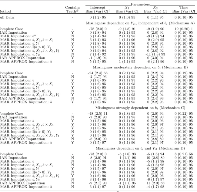
Table S1 shows the simulation results. Complete case analysis produced biased pa-rameter estimates in all four underlying missingness mechanisms considered. Under MAR missingness mechanism (A), the MAR-based imputation approach produces unbiased pa-rameter estimates. LMAR imputation under mechanism (A) produces biased papa-rameter estimates when an incorrect working missingness model is used. When the working model contains the underlying missingness model, however, the LMAR method results in essen-tially unbiased parameter estimates. Under mechanism (A), the MAR-based imputation approach and the LMAR imputation approach with the correct working model result in very similar coverage and relative variance. APPROX Imputation using a logistic
re-gression model for imputingX2 had similar performance to imputation using kernel (4).
This suggests that the LMAR-based imputation approach can be applied when the true missingness model is MAR as long as the missingness model contains the true model.
Under mechanism (B), all imputation approaches produce essentially unbiased or low bias parameter estimates. The LMAR approaches, however, result in small increases in coverage and reductions in variance and bias compared to the MAR imputation approach. Under mechanism (C), the MAR-based imputation approach produces noticeable bias in estimating the mixed model intercept and parameter associated with the imputed covari-ate. We see corresponding reductions in coverage for these parameters. In contrast, the LMAR-based imputation approaches produce unbiased parameter estimates. For
mecha-nisms (B) and (C), the working model that usesI(b >0) instead ofbin the working model
still shows good performance despite the fact that the working model does not contain the true model. We do not see evidence of problems arising from lack of identifiability or lack of convergence under any of the working models considered here. MAR-based
imputation using a logistic regression model for imputing X2 resulted in slightly greater
bias than MAR imputation using kernel (4).
Under mechanism (D), MAR-based imputation was substantially biased, and all im-putation settings assuming LMAR-based imim-putation resulted in reduced bias. Notably, even in imputation settings where the missingness model was mis-specified (truth depends
linearly on b and Y1), we can see a reduction in bias compared to MAR-based
imputa-tion. Taken as a whole, this set of simulations suggests that our imputation approach can induce bias when the missingness model is far off the true model, but we can often see good properties when the working model contains or is somewhat “close” to the true model.
Table S1: Linear mixed model estimates using proposed imputation methods Parameters
Contains Intercept X1 X2 Time
Method Truth# Bias (Var) CI† Bias (Var) CI Bias (Var) CI Bias (Var) CI
Full Data - 0 (1.2) 95 0 (1.0) 95 0 (1.1) 95 0 (0.10) 95
Missingness dependent onYi1, independent ofbi(Mechanism A)
Complete Case - -78 (2.0) 0 -9 (1.8) 91 -9 (1.9) 90 19 (0.20) 1 MAR Imputation Y 0 (1.8) 94 0 (1.1) 95 0 (2.8) 94 0 (0.10) 95 LMAR Imputation: b* N 6 (1.4) 94 2 (1.1) 95 -9 (1.9) 94 0 (0.10) 95 LMAR Imputation: b, X1, b×X1 N 6 (1.4) 93 1 (1.1) 96 -9 (2.0) 95 0 (0.10) 95 LMAR Imputation: b, Y1 Y 0 (1.8) 94 0 (1.1) 96 0 (2.8) 94 0 (0.10) 95 LMAR Imputation: I(b >0), Y1 Y 0 (1.9) 94 0 (1.1) 96 0 (2.8) 93 0 (0.10) 95 LMAR Imputation: b, X1, b×X1, Y1 Y 0 (1.9) 94 0 (1.1) 95 0 (2.8) 92 0 (0.10) 95 LMAR Imputation: b, Y2 N 7 (1.4) 92 2 (1.1) 95 -11 (1.8) 93 0 (0.10) 95
MAR APPROX Imputation Y -1 (1.9) 94 0 (1.1) 96 0 (3.0) 94 0 (0.10) 95
LMAR APPROX Imputation: b N 5 (1.5) 95 1 (1.1) 95 -8 (2.1) 96 0 (0.10) 95
Missingness moderately dependent onbi(Mechanism B)
Complete Case - -24 (2.4) 66 0 (2.1) 95 0 (2.2) 94 0 (0.19) 95 MAR Imputation N -2 (1.7) 93 0 (1.1) 95 2 (2.4) 92 0 (0.10) 95 LMAR Imputation: b Y 0 (1.6) 95 0 (1.1) 95 0 (2.2) 93 0 (0.10) 95 LMAR Imputation: b, X1, b×X1 Y 0 (1.6) 95 0 (1.1) 95 0 (2.2) 94 0 (0.10) 95 LMAR Imputation: b, Y1 Y 0 (1.6) 95 0 (1.1) 95 0 (2.2) 94 0 (0.10) 95 LMAR Imputation: I(b >0), Y1 N 0 (1.6) 95 0 (1.1) 95 0 (2.2) 94 0 (0.10) 95 LMAR Imputation: b, X1, b×X1, Y1 Y 0 (1.6) 95 0 (1.1) 95 0 (2.2) 94 0 (0.10) 95
MAR APPROX Imputation N -3 (1.7) 94 0 (1.1) 95 3 (2.4) 93 0 (0.10) 95
LMAR APPROX Imputation: b Y 0 (1.6) 95 0 (1.1) 95 0 (2.2) 95 0 (0.10) 95
Missingness strongly dependent onbi(Mechanism C)
Complete Case - -48 (2.5) 11 0 (1.8) 95 0 (2.0) 94 0 (0.22) 95 MAR Imputation N -7 (2.0) 90 0 (1.1) 95 8 (2.8) 90 0 (0.10) 95 LMAR Imputation: b Y 0 (1.5) 96 0 (1.1) 96 0 (2.0) 96 0 (0.10) 95 LMAR Imputation: b, X1, b×X1 Y 0 (1.5) 96 0 (1.1) 96 0 (2.0) 97 0 (0.10) 95 LMAR Imputation: b, Y1 Y 0 (1.6) 95 0 (1.1) 95 0 (2.1) 95 0 (0.10) 95 LMAR Imputation: I(b >0), Y1 N 0 (1.6) 95 0 (1.1) 96 0 (2.1) 96 0 (0.10) 95 LMAR Imputation: b, X1, b×X1, Y1 Y 0 (1.5) 96 0 (1.1) 96 0 (2.1) 96 0 (0.10) 95
MAR APPROX Imputation N -8 (2.0) 90 0 (1.1) 95 9 (2.8) 89 0 (0.10) 95
LMAR APPROX Imputation: b Y 0 (1.5) 97 0 (1.1) 96 0 (2.1) 97 0 (0.10) 95
Missingness dependent onbiandYi1 (Mechanism D)
Complete Case - -73 (2.0) 0 -5 (1.6) 93 -5 (1.6) 94 8 (0.21) 56 MAR Imputation N -8 (2.0) 91 -1 (1.1) 96 10 (2.8) 89 0 (0.10) 95 LMAR Imputation: b N 3 (1.4) 96 0 (1.1) 96 -5 (1.7) 98 0 (0.10) 95 LMAR Imputation: b, X1, b×X1 N 3 (1.4) 96 0 (1.1) 96 -5 (1.6) 98 0 (0.10) 95 LMAR Imputation: b, Y1 Y 0 (1.5) 97 0 (1.1) 96 0 (2.0) 97 0 (0.10) 95 LMAR Imputation: I(b >0), Y1 N 0 (1.6) 96 0 (1.1) 96 0 (2.0) 97 0 (0.10) 95 LMAR Imputation: b, X1, b×X1, Y1 Y 0 (1.6) 96 0 (1.1) 96 0 (2.0) 96 0 (0.10) 95 LMAR Imputation: b, Y2 N 3 (1.4) 96 0 (1.1) 95 -6 (1.7) 97 0 (0.10) 95
MAR APPROX Imputation N -9 (2.1) 90 -1 (1.1) 95 11 (2.9) 88 0 (0.10) 95
LMAR APPROX Imputation: b N 3 (1.4) 97 0 (1.1) 96 -4 (1.7) 98 0 (0.10) 95
*Variables after colon represent linear predictors in working model forRDi
†All values in table multiplied by 100. CI indicates coverage of 95% confidence intervals. Var indicates empirical variance.
# Indicates whether working missingness model contains true model.
APPROX: Imputation ofX2 uses a logistic regression with predictorsX1, b, Y1, Y2, Y3(instead of kernel (4))
S4.2
Simulation 2: Cox proportional hazards mixture cure model
We simulate 500 datasets of 500 subjects under a CPH mixture cure model. Covariates
X1 and X2 are simulated as in Simulation 1. We simulate an underlying cure status
using the relation logit(P(Not Cured|Xi1, Xi2)) = 0.5 + 0.5Xi1 + 0.5Xi2. This results
in an average cure rate of 26%. For the non-cured group (G=1), we simulate an event
time using the hazard function λ(t) = 0.0005t0.3e0.5Xi1+0.5Xi2. For cured subjects (G=0),
the event time is taken to be infinity. We generate censoring times using the relation
λC(t) = 0.00015t0.5 for the first 400 subjects and impose administrative censoring at
3000 for the remaining 100 subjects. The observed event/censoring time Ti is taken as
the minimum of the censoring and event time, and δi represents the event indicator. In
this simulation setting, Y = (T, δ), X = (X1, X2), and L = G. For the estimation, we
assume subjects with Ti greater than a late cut-point are cured. We choose a cut-point
of 50 as the Kaplan-Meier plots demonstrate a clear plateau by that point. We impose
∼50% missingness in X2 using each of the following mechanisms:
(A) MCAR with missingness probability of 0.5
(B) LMAR with logit(P(X2 missing|X1, G, T, δ)) =−0.2 + 0.3G
(C) LMAR with logit(P(X2 missing|X1, G, T, δ)) =−0.9 + 1.2G.
(D) LMAR with logit(P(X2 missing|X1, G, T, δ)) =−1.1 + 1.2G+ 0.5X1.
Mechanism (A) is MCAR, mechanism (B) is LMAR with a moderate dependence on
cure status (G), mechanism (C) is LMAR with a strong dependence on cure status, and
mechanism (D) depends on both cure status and X1.
We assume a Weibull baseline hazard in the non-cured group for imputation. For each imputed dataset, we fit a CPH cure model, which consists of a logistic regression for the probability of not being cured and a Cox regression for the hazard of events in
the not cured group. We fit this model using the packagesmcure in R (Cai et al., 2012).
Variances were estimated using 100 bootstrap samples.
Table S2 shows the simulation results for the Cox proportional hazards mixture cure model. As expected, complete case analysis is essentially unbiased under covariate miss-ingness mechanism (A) (MCAR), but the imputation-based methods are more efficient than the complete case analysis. When missingness depends on the underlying cure sta-tus, however, complete case analysis is biased. We see comparatively little bias in the imputation-based estimates across missingness mechanisms and imputation models us-ing kernel (4). We note that even when we specify the correct missus-ingness model, we sometimes see bias in estimating the intercept parameter in the logistic regression. This parameter is the most difficult to estimate due to identifiability issues with the CPH cure model, and these biases will reduce with larger sample sizes (simulated sample size = 500). As such, we should not over-interpret bias in this parameter. APPROX Imputation using
a logistic regression model for imputingX2 resulted in increased bias in all scenarios. For
missingness mechanisms (A) and (B) and using kernel (4) for imputation, we see very little difference between the MAR and LMAR imputation approaches in terms of bias, coverage, and relative variance. APPROX imputation under LMAR resulted in slightly larger variances than APPROX imputation under MAR.
In mechanism (C) (when missingness depends strongly on cure status) and
mecha-nism (D) (when missingness depends on cure status and X1), we still see little difference
between MAR and LMAR imputation methods using kernel (4) in terms of bias. Larger bias differences between MAR-based and LMAR-based imputation can be seen when co-variate imputation uses a logistic regression instead of kernel (4) in mechanism (c). The LMAR imputation approaches using kernel (4) (which differ only in terms of the work-ing misswork-ingness model) produce essentially unbiased estimates for all model parameters
G×X1 in the working model resulted in some numerical convergence issues for several of the simulations (15 simulations failed), which may indicate issues with model identifi-ability (possibly due to collinearity). We included only the converging simulations (485
of them) in Table S2.
Overall, these simulations suggest a large degree of stability in CPH cure model in-ference when we impute assuming MAR and the true mechanism is LMAR. A greater degree of bias is introduced in the APPROX simulations, where the covariate imputation distribution assumed to follow a simple regression model form rather than the form in (4).
T able S2: CPH cure mo del estimates using p rop osed imputation metho ds -Logistic Regression -Co x Regression -Con tains In tercept X1 X2 X1 X2 Metho d T ruth # Bias (V ar) CI Bias (V ar) CI Bias (V ar) CI Bias (V ar) CI Bias (V ar) CI F ull Data -1 (6.5) 94 1 (7.9) 95 0 (8.4) 95 0 (2.0) 95 0 (2.3) 95 MCAR missingness indep end e n t of Gi (Mec hanism A) Complete Cas e -2 (12.7) 97 1 (14.9) 97 1 (18.5) 96 1 (4.3) 95 0 (5.1) 94 MAR Imputation Y 3 (9.1) 94 1 (8.4) 96 0 (18.0) 95 0 (2.1) 96 0 (4.8) 93 LMAR Imputation: G * Y 3 (9.4) 94 1 (8.3) 96 0 (19.5) 95 0 (2.1) 96 0 (4.9) 94 LMAR Imputation: G, X 1 , Y , δ Y 3 (9.3) 94 1 (8.3) 96 0 (18.8) 95 0 (2.1) 96 0 (4.8) 95 LMAR Imputation: G, X 1 , G × X1 Y 3 (9.5) 94 1 (8.4) 96 0 (18.9) 95 0 (2.1) 96 0 (4.8) 95 MAR APPR O X Imputation Y 6 (9.4) 93 1 (8.2) 95 -6 (19.6) 91 0 (2.1) 96 -1 (4.4) 93 LMAR APPR O X Imputation: G Y 6 (9.6) 93 1 (8.4) 96 -6 (21.1) 91 0 (2.1) 96 -2 (4.5) 91 Missingness mo derately d e p enden t on Gi (Mec hanism B) Complete Cas e --13 (12.1) 93 3 (16.0) 97 0 (15.4) 97 0 (4.8) 9 5 1 (5.4) 93 MAR Imputation N 3 (8.8) 95 0 (8.5) 96 0 (16.9) 96 0 (2.2) 96 0 (4.8) 93 LMAR Imputation: G Y 3 (8.9) 96 0 (8.5) 96 0 (16.7) 96 0 (2.2) 95 0 (4.8) 94 LMAR Imputation: G, X 1 , Y , δ Y 3 (8.8) 94 1 (8.5) 96 0 (16.0) 96 0 (2.2) 95 1 (4.7) 94 LMAR Imputation: G, X 1 , G × X1 Y 3 (9.0) 94 0 (8.6) 96 0 (16.3) 95 0 (2.2) 95 0 (4.8) 93 Missingness strongly dep enden t on Gi (Mec hanism C) Complete Cas e --50 (9.9) 62 2 (12.9) 97 0 (12.2) 96 1 (5.4) 95 0 (5.8) 95 MAR Imputation N 4 (8.3) 96 1 (8.6) 96 -1 (15.2) 95 0 (2.2) 96 0 (5.1) 94 LMAR Imputation: G Y 2 (7.9) 95 0 (8.5) 97 0 (13.3) 96 0 (2.3) 96 0 (5.5) 93 LMAR Imputation: G, X 1 , Y , δ Y 2 (7.8) 95 1 (8.4) 97 1 (13.0) 96 0 (2.2) 95 0 (5.4) 93 LMAR Imputation: G, X 1 , G × X1 Y 1 (7.5) 93 1 (8.1) 94 0 (13.0) 93 0 (2.2) 92 0 (5.4) 91 MAR APPR O X Imputation N 8 (8.4) 93 1 (8.5) 97 -12 (16.1) 91 0 (2.3) 96 -1 (5.3) 90 LMAR APPR O X Imputation: G Y 6 (8.0) 94 1 (8.4) 97 -9 (14.2) 93 1 (2.3) 96 -1 (5.2) 91 Missingness dep enden t on Gi and Xi 1 (Mec hanism D) Complete Case --45 (9.1) 69 -12 (13.1) 96 0 (12.0) 96 1 (5.6) 95 0 (6.5) 95 MAR Imputation N 4 (8.4) 95 0 (8.5) 97 -2 (15.5) 94 0 (2.3) 96 0 (5.6) 94 LMAR Imputation: G, X 1 Y 3 (7.8) 95 0 (8.5) 98 0 (13.2) 96 0 (2.3) 96 0 (6.0) 93 *V ariables after colon represen t linear predictors in w orking mo del for R D i † All v alues m ultiplied b y 100. CI indicates co v erage of 95% confidence in terv als. V ar indicates empirical v ariance. # Indicates whether w orking missingness mo del con tains true mo del. APPR O X: Imputation of X2 uses a logistic regression with predictors X1 , G, G × H0 ( Y ) , G × H0 ( Y ) × X1 .
S4.3
Simulation 3: mixture of normals
We simulate 500 datasets of 500 subjects under a normal mixture model with two binary
covariates and two latent classes. CovariatesX1 andX2 are simulated as in Simulation 1.
We generate the mixing variableCi withP(Ci = 1) = 0.62 for each individual. We draw
N(0,1) errors ei and then generate Y using the model Yi = 0.5 + 0.5Xi1 + 0.5Xi2+ei if
Ci = 1 and Yi = 2 + 3Xi1+ 2Xi2+ei if Ci = 0. In this simulation setting,X = (X1, X2)
and L=C. We then impose missingness inX2 using each of the following mechanisms:
(A) MAR withP(X2 missing|X1, C, Y) =−0.5 + 0.2Y
(B) LMAR with P(X2 missing|X1, C, Y) =−0.3 + 0.5C
(C) LMAR with P(X2 missing|X1, C, Y) = −1.1 + 1.7C.
Mechanism (A) is MAR dependent on Y. Mechanism (B) is LMAR with a moderate
dependence on the latent class variable (C), and mechanism (C) is LMAR with a strong
dependence on the latent class.
For each imputed dataset, we fit a latent class model (with two classes) using the
package ‘flexmix’ in R to estimate θ through an EM algorithm (Leisch, 2004). The
pack-age ‘flexmix’ estimates the variance for ˆθ for each dataset by fitting a GLM weighted
by estimated class membership probabilities for each individual. When parameters are
drawn using latent class modeling, we may not be able to determine which value of C
belongs to which subclass identified by the latent class modeling. In other words, we may
not be able to differentiate which subset of θ belongs to which value of C. We can
cir-cumvent this issue by placing an additional assumption to differentiate between classes.
We impose an identifying restriction that defines class Ci = 1 to be the cluster
deter-mined by the latent class modeling with a smaller intercept value. We note that the two clusters are well-separated in this example. We predict that we may encounter greater identifiability issues (in differentiating the clusters) when the clusters have parameters that are very close together.
Table S3 shows the simulation results for a mixture of normal distributions. Com-plete case analysis results in biased parameter values for mechanism (A) and mild or no bias for mechanisms (B) and (C). For mechanism (A), the MAR-based imputation approach produces essentially unbiased parameter estimates. The LMAR imputation approaches with working missingness models containing the true missingness model also produce very small bias. Mild increases in bias can be seen for the LMAR imputation approach using an incorrect working model. Compared to the MAR approach, the LMAR approach using the correct working model resulted in similar or slightly larger variances for all parameter estimates.
For mechanism (B), little bias can be seen across all of the imputation approaches. Similar coverage rates can be seen across imputation approaches. In this example, we see slightly smaller variances for the LMAR approaches with the more complicated working models. Under mechanism (C), we see increases in bias and small decreases in cover-age for estimating mixture model parameters using the MAR-based imputation method
(either using kernel (4) or logistic regression for imputing X2). The LMAR-based
im-putation method using only C in the working missingness model produces essentially
unbiased parameter estimates for all parameters. Compared to the approaches using the more complicated working model, the simpler LMAR approach using kernel (4) results in smaller variances for estimating model parameters.
T able S3: Mixture of normals mo del estimates using prop osed imputation metho ds -C = 1 -C = 0 -Con tains In tercept X 1 X 2 In tercept X1 X2 Metho d T ruth # Bias (V ar) CI Bias (V ar) CI Bias (V ar) CI Bias (V ar) CI Bias (V ar) CI Bias (V ar) CI F ull Data -0 (1.6) 95 0 (1.9) 92 0 (1.5) 97 0 (3.6) 94 0 (3.3) 94 0 (3.4) 94 Missingness dep enden t on Yi , indep enden t of Ci (Mec hanism A) Complete Cas e -2 (2.8) 94 -7 (3.5) 92 -4 (2. 7) 95 3 (12. 6) 93 -12 (10.3) 90 -4 (10.3) 93 MAR Imputation Y 1 (1.9) 95 0 (4.3) 94 1 (4.6) 95 -1 (6.1) 94 -2 (7.8) 94 0 (5.5) 95 LMAR Imputation: C * N 3 (1.9) 94 1 (4.6) 94 -2 (4.5) 95 -3 (6.2) 94 -4 (7.8) 94 2 (5.6) 94 LMAR Imputation: C , Y , X 1 Y 1 (2.0) 94 0 (4.3) 93 1 (4.6) 95 -1 (6.4) 95 -2 (7. 7 ) 94 0 (5.3) 95 LMAR Imputation: C , Y , C × Y Y 1 (2.0) 94 1 (4.6) 93 1 (4.6) 96 -2 (6.2) 94 -2 (8. 1 ) 94 0 (6.0) 95 LMAR Imputation: C , Y , C × Y ,X 1 Y 1 (2.0) 94 0 (4.5) 93 1 (4.9) 95 -2 (6.3) 94 -2 (8. 0) 93 0 (6.0) 94 MAR APPR O X Imputation Y 1 (2.0) 94 0 (2.9) 93 0 (3.2) 92 0 (6.3) 92 0 (6.4) 93 -3 (5.5) 94 LMAR APPR O X Imputation: C N 3 (1.9) 93 0 (3.4) 93 -3 (3.8) 93 -1 (6.3) 93 -2 (6.9) 92 0 (5.3) 93 Missingness mo derately d e p enden t on Ci (Mec hanism B) Complete Cas e -1 (5.4) 93 -1 (5.4) 93 0 (4.1) 95 -1 (8.6) 91 0 (7.9) 92 0 (6.9) 91 MAR Imputation N 1 (2.3) 94 0 (2.7) 94 -1 (4.0) 93 -2 (5.8) 94 -2 (4.8) 95 2 (4.7) 93 LMAR Imputation: C Y 0 (2.3) 94 1 (4.7) 94 1 (5.1) 93 -1 (5.6) 95 -2 (6. 4) 95 0 (5.3) 94 LMAR Imputation: C , Y , X 1 Y 0 (2.4) 95 1 (5.1) 94 1 (5.5) 93 -1 (5.8) 94 -2 (7. 1) 95 0 (5.7) 93 LMAR Imputation: C , Y , C × Y Y 0 (2.4) 94 1 (3.8) 94 1 (4.9) 92 -1 (5.7) 93 -2 (5. 7) 94 0 (5.0) 94 LMAR Imputation: C , Y , C × Y ,X 1 Y 1 (2.4) 95 1 (3.6) 95 1 (4.7) 92 -1 (5.8) 94 -2 (5. 6) 94 0 (5.0) 94 Missingness strongly dep enden t on Ci (Mec hanism C) Complete Cas e -3 (8.2) 93 -2 (7.6) 92 -1 (6.4) 93 -2 (5.8) 92 1 (6.1) 92 1 (5.3) 92 MAR Imputation N 5 (2.5) 93 2 (7.2) 93 -7 (7.4) 91 -5 (4.9) 95 -4 (7.6) 94 5 (7.0) 92 LMAR Imputation: C Y 1 (2.8) 94 1 (4.6) 94 0 (6.4) 92 -1 (4.5) 96 -2 (5. 9) 95 0 (5.2) 94 LMAR Imputation: C , Y , X 1 Y 1 (2.9) 94 2 (5.9) 94 0 (7.2) 92 -2 (4.7) 96 -3 (6. 9) 95 0 (5.9) 94 LMAR Imputation: C , Y , C × Y Y 1 (2.8) 94 1 (5.4) 94 0 (7.3) 92 -2 (4.5) 96 -2 (6. 7) 95 0 (5.8) 93 LMAR Imputation: C , Y , C × Y ,X 1 Y 1 (2.8) 95 2 (6.6) 94 0 (7.8) 92 -2 (4.8) 94 -3 (8. 0) 94 0 (6.1) 92 MAR APPR O X Imputation N 5 (2.5) 92 2 (5.7) 93 -7 (6.6) 88 -6 (4.9) 94 -3 (6.8) 94 6 (6.2) 91 LMAR APPR O X Imputation: C Y 1 (2.8) 92 2 (6.6) 94 0 (7.3) 87 -1 (4.4) 95 -3 (7. 3) 95 0 (6.4) 94 *V ariables after colon represen t linear predictors in w orking m o del for R D i † All v alues in table m ultiplied b y 100. CI indicates co v erage of 95% confidence in terv als.V ar indicates empirical v ariance. # Indicates whether w orking missingness mo del con tains true mo del. APPR O X: Imputation of X 2 uses a logistic regression with predictors C , X1 , X1 × C , Y , Y × C (instead of k ernel (4))
S4.4
Simulation 4: Exploring identifiability and convergence
One criticism of the selection model factorization in (1) is that it is often difficult to de-termine whether the parameters of the working missingness model are identifiable (Little, 2009). By “identifiable,” we mean that the observed data likelihood has a unique maxi-mizer. Even if the model parameters are technically identifiable, one additional concern is that the likelihood surface near the maximizer may be nearly flat. These identifiability concerns can lead to issues with model fitting and convergence of the imputation algo-rithm. In order to better understand possible identifiability-related convergence issues, we perform a set of simulations evaluating convergence of the imputation algorithm under a variety of modeling scenarios.
We simulate 500 complete datasets under a linear mixed model, cure model, and
mixture of normals as in Simulations 1-3. We impose ∼50% covariate or outcome
miss-ingness (but not both) under a variety of missmiss-ingness models.
For covariate missingness, we generate MAR and LMAR missingness using missing-ness mechanisms (A) and (C) from Simulations 1-3. For both the linear mixed model and mixture of normals model, we generate outcome missingness under MCAR and LMAR using mechanism (C) from Simulations 1 and 3 applied to the outcome instead of the covariate. We also impose LMAR outcome missingness for the mixture of normals model
using the relation logit(P(Y missing|X, C)) =−1.1 + 0.5X1−0.5X2+ 1.7C. This results
in ∼50% outcome or covariate missingness in each scenario. We note that in each case
in Simulation 4, we only have missingness in a single covariate (X2) or a single outcome
variable (Y). Therefore, the SMC imputation distributions do correspond to a valid joint
model, although that joint model was never specified directly. The primary purpose of this simulation is to explore identifiability-related convergence issues, which would be similarly present in the joint modeling and SMC imputation settings.
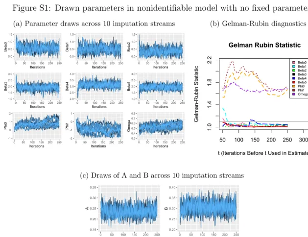
For each outcome model parameter, we estimate the fraction of missing information as described in (Little and Rubin, 2002). We also calculate the Gelman-Rubin convergence statistic (the potential scale reduction factor) for the outcome and missingness model parameter draws across imputation streams. The Gelman-Rubin statistic is a measure of the relative between and within-chain variance, and values less than 1.1 generally indicate satisfactory convergence (Gelman and Rubin, 1992). We also calculate a multivariate ver-sion of the Gelman-Rubin statistic to evaluate convergence overall across different model parameters (Brooks and Gelman, 1998).
Table S4 shows the simulation results. Under covariate missingness, the fractions of missing information tend to be generally small, particularly for parameters related to
X1, the fully-observed covariate. We see larger estimates for the fraction of missing
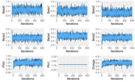
in-formation when we impose similar rates of missingness in the outcome. Additionally, we see good Gelman-Rubin convergence properties under covariate missingness and MAR outcome missingness. Under LMAR outcome missingness, the outcome model parame-ters appear to converge, but the parameparame-ters in the missingness model (in particular, the parameter attached to the latent variable) show some evidence of convergence problems. The drawn values of the outcome model parameters appear reasonable (with small or no bias) even when the missingness model parameters do not converge, but this may not be true in general. When we fix the value of the parameter related to the latent variable in the missingness, we see a large improvement in the convergence properties of the imputation algorithm.
T able S4: F raction of missing information and co n v ergence prop erties † —– F raction of Missing Information —– ——————–Gelman-Rubin Statistic ——————– Ov erall Outcome Mo del P arameters* Outcome Mo del P arameters* φ † 0 φ ‡ 1 Gelman-Rubin Co v ariate missingness Linear Mixed Mo del, MAR 0.27 0.07 0.54 0 1.01 1.00 1.02 1.01 -1.03 Linear Mixed Mo del, LMAR: b # 0.24 0.06 0.52 0 1.01 1.00 1.01 1.01 1.00 1.03 1.04 Cure Mo del, MCAR 0.20 0.03 0.46 0.06 0.45 1.01 1.00 1.02 1.00 1.01 -1.04 Cure Mo del, LMAR: G 0.16 0.02 0.36 0.07 0.52 1.01 1.00 1.01 1.00 1.02 1.00 1.00 1.04 Mixture of Normals, MAR 0.17 0.06 0.39 0.39 0.32 0.32 1.00 1.02 1.01 1.00 1.01 1.01 -1.02 Mixture of Normals, LMAR: C 0.33 0.10 0.62 0.22 0.14 0.14 1.00 1.02 1.01 1.00 1.01 1.00 1.00 1.01 1.02 Outcome miss in gnes s Linear Mixed Mo del, MCAR 0.18 0.22 0.21 0.49 1.00 1.01 1.01 1.03 -1.05 Linear Mixed Mo del, LMAR: b 0.19 0.22 0.20 0.57 1.01 1.01 1.01 1.07 1.00 1.10 1.14 Linear Mixed Mo del, LMAR: b 0.18 0.21 0.22 0.52 1.01 1.01 1.01 1.04 1.01 FIXED 1.06 Mixture of Normals, MCAR 0.52 0.54 0.53 0.54 0.54 0.54 1.02 1.03 1.02 1.02 1.02 1.01 -1.06 Mixture of Normals, LMAR: C 0.57 0.57 0.57 0.46 0.46 0.47 1.02 1.02 1.01 1.01 1.03 1.01 1.55 1.65 1.66 Mixture of Normals, LMAR: C , X 0.58 0.62 0.57 0.47 0.48 0.47 1.02 1.02 1.02 1.01 1.03 1.01 1.38 1.64 1.65 Mixture of Normals, LMAR: C 0.68 0.68 0.66 0.35 0.35 0.35 1.04 1.04 1.02 1.01 1.03 1.01 1.05 FIXED 1.13 Mixture of Normals, LMAR: C , X 0.67 0.71 0.65 0.35 0.37 0.34 1.04 1.03 1.02 1.01 1.03 1.01 1.01 FIXED 1.08 † Imputations dra wn using k ernels (2)–(3) *F or eac h mo del, these are the parameters from the outcome mo del (same as T ables S 1 -S3 ): —– Linear mixed mo del: in tercept, X1 , X2 , and time —– Cure mo del: in tercept, X 1 , and X2 in the logistic regression and X1 and X2 in the Co x regression —– Mixture of Normals: in te rc ept, X1 , and X 2 for the C = 1 and C = 0 classes resp ectiv ely ‡ φ0 is the in tercept in the missingness mo del. φ1 is the parameter for the laten t v ariab le . # Notation: T rue and w orking mis sin g n e ss mo dels dep end on v ariables after c olon
S4.5
Simulation 5: Comparison of final analysis with and
with-out imputed
L
After imputation, we have several choices as to what combination of the imputed L and
D we want to include in the final analysis. We first suppose that we will perform our
final analysis ignoring the contribution of R. When both imputedD and Lare included
in the final analysis, R is ignorable. In Property 4, we show that R is also ignorable if
only imputed D is included in the final analysis when missingness is MAR. When
miss-ingness is LMAR, we show in Property 5 that final analysis using only the imputed D
and ignoring R will be valid but not fully efficient. In this section, we want to briefly
explore the practical impact of including or excluding the imputed values ofL (assuming
we are ignoringR) in the final analysis through simulation.
We generate simulated data under a linear mixed model, mixture of normals model, and Cox proportional hazards model as described for Simulations 1-3. We impose
ei-ther MAR or LMAR (Strong Dependence) missingness in X2 as in Simulations 1-3 and
impute using a working missingness model with the correct structure (either MAR or LMAR dependent only on the latent variable) and kernels (2)–(4). After imputation, we
perform the final analysis using the imputed values for X2 and either ignoring or using
the imputed values for the latent variable (and in both cases ignoring R). Additionally,
in the course of our simulations, we observed that some simulations under the mixture of normals model had estimated variances that were very large when we used the imputed latent variable in the final model fit. This may be an indicator of inadequate convergence of the model fit. Therefore, we present the mixture of normals results 1) for all 500 sim-ulations and 2) restricting to simsim-ulations in which the estimated variances were all less than 0.2 (20 in the scale presented in the table). This issue did not arise for the linear
mixed model simulations. In Tables S1-S3, we perform all final analyses ignoring the
imputed latent variable and without restricting to simulations that have variance < 0.2,
and the corresponding rows in this table are the same as the results in Tables S1-S3.
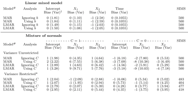
Table S5 shows the simulation results. We first consider the results for the mixture of normals model. We first notice that analyses using the imputed latent variable in the final analysis result in substantial bias when we include all simulations in our estimation of bias. This is the result of just a few simulations with parameter estimates far from the true value. This suggests some instability or lack of convergence in the model fitting. However, when we restrict our focus to simulations that appear to have convergence (rea-sonable standard errors), we see that final analyses including and excluding the imputed latent variable perform similarly well. For some simulation settings, the variance
esti-mates using C are slightly larger, and the reverse is true for other simulations, so there
is not a clear trend in efficiency including or excluding the latent variable in the final analysis in these simulations.
Although not included in our results, it is worth mentioning that analysis including
and ignoring the imputed L may be associated with different fractions of missing
infor-mation, which could have implications on the number of imputations needed for good
inference. Let ¯U represent the average of the variance estimators for parameter θ across
the mimputed datasets and B represent the sample variance of the estimates of θ across
the m imputed datasets. Then, we can express the relative increase in variation due to
The relative efficiency of an estimateθbased onmimputations compared to the estimate based of in infinite number of imputations is:
RE = 1
1 + λ
m
We may expect an analysis that conditions on the imputedLin the final analysis to have
larger relative between imputation variance vs. within imputation variance (r) compared
to an analysis that does not condition on L in the final analysis for some parameters.
This is because, when we include Lin the final analysis, each fit treats the imputed Las
known, resulting in substantially reduced “within imputation” standard error estimates for some parameters. This leads to larger values for the fraction of missing information,
λ, for the same value ofmwhen we includeLin the final analysis compared to an analysis
that ignores imputed L. In simulations (not shown), a final analysis using L did result
in larger fractions of missing information compared to an analysis ignoring imputed L
in the random intercept linear mixed model setting. We note that in practice this may translate into only a very small difference in relative efficiency between the two methods of analysis. However, several authors have noted practical issues regarding estimation of p-values and confidence intervals when a small number of imputations are used and the fraction of missing information is moderate to large (e.g. White and Royston, 2011; Bodner, 2008). Therefore, we may prefer to perform our final analysis using only the
imputed D in the final analysis in an attempt to reduce the potential negative impact of
larger fractions of missing information.
Table S5: Bias and variance of parameter estimates under different final analyses
Linear mixed model
Model# Analysis Intercept X
1 X2 Time SIMS
Bias (Var)† Bias (Var) Bias (Var) Bias (Var)
MAR Ignoringb 0 (1.81) 0 (1.10) -1 (2.58) 0 (0.1055) 500 MAR Usingb 0 (1.84) 0 (1.11) -1 (2.59) 0 (0.1055) 500 LMAR Ignoringb 0 (1.49) 0 (1.15) -1 (2.03) 0 (0.1055) 500 LMAR Usingb 0 (1.50) 0 (1.08) -1 (2.05) 0 (0.1055) 500 Mixture of normals - - - C = 1- - - C = 0 - - - SIMS
Model# Analysis Intercept X
1 X2 Intercept X1 X2
Bias (Var) Bias (Var) Bias (Var) Bias (Var) Bias (Var) Bias (Var)
Variance Unrestricted MAR IgnoringC 1 (1.98) 0 (4.35) 1 (4.64) -1 (6.18) -2 (7.80) 0 (5.53) 500 MAR UsingC 2 (2.22) 6 (7.55) 5 (6.38) -3 (7.09) -8 (10.38) -3 (6.49) 500 LMAR IgnoringC 1 (2.89) 1 (4.63) 0 (6.42) -1 (4.56) -2 (5.91) 0 (5.29) 500 LMAR UsingC 1 (3.28) 9 (9.71) 5 (7.76) -3 (5.18) -9 (10.03) -4 (7.18) 500 Variance Restricted* MAR IgnoringC 1 (2.04) -1 (2.09) 0 (2.88) -1 (6.06) 0 (5.34) 0 (5.02) 483 MAR UsingC 1 (2.07) -1 (1.95) 0 (2.94) 0 (5.73) -1 (5.14) 0 (4.25) 404 LMAR IgnoringC 0 (2.79) 0 (2.07) 0 (5.39) 0 (4.28) 0 (3.77) 1 (3.94) 477 LMAR UsingC 0 (2.95) 0 (2.11) 0 (5.44) 0 (4.35) -1 (3.75) 0 (3.95) 418
†All values in table multiplied by 100
# Indicates true and working missingness model
* Ignoring simulations in which the estimated variance was greater than 0.2 (20 in the scale of this table) for at least one parameter.
S4.6
Simulation 6: more explorations for the CPH cure model
Suppose missingness is LMAR but that we impute incorrectly assuming MAR missing-ness. Since missingness is MNAR, we may have bias in estimating the resulting model parameters when we impute assuming MAR. This bias can be seen for missingness mech-anisms strongly dependent on the latent variable in Simulations 1 (linear mixed model) and 3 (mixture of normals). In Simulation 2, however, MAR-based imputation under true LMAR missingness does not appear to create much bias in the resulting outcome model parameter estimates. In this section, we provide some intuition as to why this might be the case.
One reason for this result has to do with the form of the imputation distribution for
Gunder LMAR. Under MAR and using notation from Section S7.3, we imputeGfrom
logit(P(Gi = 1|Xi, Ti, δi = 0;ρ)) =ω0+ω1Xi−Λ0(Ti)eθXi
and we imputeG from the following under LMAR:
logit(P(Gi= 1|Xi, Ti, δi= 0, Ri;ν)) =ω0+ω1Xi−Λ0(Ti)eθXi+ log " f(R−Si |Ti, δi= 0, Xi(obs), Gi= 1;φ−S) f(R−Si |Ti, δi= 0, X (obs) i , Gi= 0;φ−S) #
These two distributions differ only by the offset term, log f(R−Si |Ti,δi=0,Xi(obs),Gi=1;φ−S) f(R−Si |Ti,δi=0,X (obs) i ,Gi=0;φ−S) . This offset term follows the familiar form of the offset term under case-control sampling
dependent on G.
Suppose first that missingness depends only on G. In this case, the two distributions
(imputation under MAR vs. LMAR) differ by a term depending only on R and φ−S.
Since R and X are independent givenG in this setting, exclusion of this offset term will
impact the intercept but may not appreciably impact the estimated covariate effects,ω1.
Therefore, the imputation distributions under MAR and LMAR are really only different in terms of the population cure rate, which is associated with the intercept in the logistic regression part of the Cox proportional hazards cure model.
Suppose instead that missingness depends on both G and observed X. In this case,
the offset term will be correlated with X, so exclusion of the offset term by incorrectly
assuming MAR could more appreciably impact the imputation distribution for G. This
in turn may more strongly impact the resulting inference. This is loosely supported by results from mechanism (D) in Simulation 2, but we still don’t see much difference be-tween MAR-based and LMAR-based imputation under LMAR in this setting.
An additional reason for similarity between the MAR-based and LMAR-based impu-tation results under true LMAR mechanisms may be the actual rate of missingness in
G (the partially latent cure status). Since the only difference between MAR-based and
LMAR-based imputation is the distribution used to impute G, we might expect the
im-putation distribution to have a bigger impact on inference when we have a larger degree
of missingness in G. Recall, subjects having an observed recurrence are known to be
non-cured (G = 1), and we assume subjects with long follow-up and no recurrence are
cured (G = 0). Therefore, it is the non-recurring subjects who are censored early that
have unknown cure status. We might expect that a heavier degree of censoring (resulting
in a greater proportion of subjects with missing G) may produce greater bias resulting
from imputing incorrectly assuming MAR. We performed an additional set of simulations (not shown) to explore how the degree of censoring impacted the relative performance of
where we might expect a lot of bias, therefore, we couldn’t even feasibly fit the model of interest, and settings in which the censoring mechanism was such that we did not run into numerical issues produced little difference between MAR-based and LMAR-based imputation.
One subtle reason for this lack-of-bias phenomenon is that LMAR-based missingness is truly a small step from MAR missingness in the cure model setting. Intuitively, we might expect some bias from incorrectly assuming MAR when missingness is LMAR.
However, one distinguishing feature of the cure model is that G is partially observed.
WhenGis observed, it is always equal to the observed event status indicator,δ. Suppose
we observed recurrences for every single non-cured subject. In this case, LMAR
missing-ness is actually MAR, sinceδrepresents the true cure status. This will usually not be the
case, but the close relationship between G and δ may be enough to protect against bias
resulting from ignoring LMAR missingness. We might think of δ as a messy measure of
G. By conditioning on δ, we might make the MAR assumption more reasonable.
While it is possible to have induced bias due to ignoring LMAR missingness in the Cox proportional hazards cure model setting, this bias resulting from ignoring the latent-dependent missingness mechanism is therefore generally expected to be somewhat small. This is demonstrated in Simulation 2 and in the analysis of the head and neck cancer data in the main paper. Although not shown, additional simulations suggest that greater amounts of censoring either do not produce much bias or create numerical issues with estimating the cure model parameters (so the data themselves are not well-suited for modeling using a cure model). We also considered different degrees of dependence be-tween missingness and cure status and fully observed covariates. In all settings explored, we still saw relatively little bias created by incorrectly assuming MAR under LMAR miss-ingness. Overall, we may be less worried about the impact of ignoring latent-dependent missingness in the Cox proportional hazards cure model setting (and possibly other set-tings with partially observed latent variables) compared do setset-tings in which the latent variable is never observed.
S5
Example 1: identifiability for joint normal models
In this paper, we restrict applications of the proposed methods to cases in which the model parameters would be identified had the missing data been observed. Here, we present an example in which parameters identified in the LMAR-based model would not be identified if the missing data had been observed. In particular, we first explore assumptions required to achieve identifiability for a measurement error model. Then, we compare the measurement error model to linear mixed models and explain how the linear mixed model is able to attain identifiability of all outcome model parameters.
S5.1
Example 1.1: Measurement Error Model with Covariates
Suppose we have a noisy version (Y) of an underlying variable of interest, L. L is never
observed, andY is observed at least for some subjects. We supposeY andLare univariate
and related to fully measured covariates, X. Suppose we model
Yi =α0+α1Li+α2Xi+ei, Li ∼N(β0+β1Xi,ΣL), ei ∼N(0, σ2), ei ⊥Li
This is an example of a measurement error model. This model contains 7 parameters. This implies the following:
Yi Li |Xi =N α0 +α1(β0+β1Xi) +α2Xi β0+β1Xi , σ2+α2 1ΣL α1ΣL α1ΣL ΣL Li|Yi, Xi ∼N β0+β1Xi+ α1ΣL σ2+α2 1ΣL [Y −α0−α1(β0+β1Xi)−α2Xi], ΣL− α21Σ2L σ2+α2 1ΣL
Suppose we have no missingness in Y. In this case, the observed data likelihood can
be expressed as follows: Lik(N oM issingobs) =
n Y i=1 f(Yi|Xi) = n Y i=1 N Yi;α0+β0α1+ [α2+α1β1]Xi, σ2+α21ΣL
whereN(a;b, c) indicates the normal density evaluated at a with meanb and variancec.
In order for the model to be identified, we must fix 4 of the 7 parameters in this
model (α0, α1, α2, σ2, β0, β1,ΣL), so we can identify the 3 remaining parameters.
Suppose instead that we have LMAR missingness in Y is follows: Probit(P(RY
i =
1|Li, Yi, Xi)) = φ0+φ1Li, so we assume that missingness in Y only depends on L. This
scenario is a simple case of the Heckman (1976) selection model if α1 = 0 with a
mod-ified missingness model (Little and Rubin, 2002; Heckman, 1976). The observed data likelihood can be expressed as follows:
Lik(obs) = n Y i=1 Z Φ(φ0+φ1Li)f(Yi, Li|Xi)dLi RYiZ (1−Φ(φ0+φ1Li))f(Li|Xi)dLi 1−RYi = n Y i=1 f(Yi|Xi) Z Φ(φ0+φ1Li)f(Li|Yi, Xi)dLi RYi 1− Z Φ(φ0+φ1Li)f(Li|Xi)dLi 1−RYi = n Y f(Yi|Xi)EL|Y,X(Φ(φ0+φ1Li))dLi RYi 1−EL|X(Φ(φ0+φ1Li)) 1−RYi
N(µ1−µ2, σ21 +σ22). Φ −p(µ1−µ2) σ2 1 +σ22 ! =P(U ≤V) = Z Φ v −µ1 σ1 fV(v)dv=EV Φ v−µ1 σ1
Using this identity and setting σ1 = 1/φ1 and that µ1 =−φ0/φ1, we have that
Lik(obs)= n Y i=1 " 1−Φ φ0+pφ1(β0+β1Xi) φ2 0+φ21ΣL !#1−RY × f(Yi|Xi)Φ φ0+φ1(β0+β1Xi) +φ1α1ΣLσ2+α21ΣL −1 (Yi−α0−α1(β0+β1Xi)−α2Xi) q φ2 0+φ21(ΣL−α12Σ2L[σ2+α 2 1ΣL] −1 ) RY
This expression contains 9 parameters, but we cannot simultaneously identify all param-eters. Suppose we set
A=φ1α1ΣL B =σ2+α21ΣL C =α0+α1β0 D =α1β1+α2
E =φ0+φ1β0 F =φ1β1 G=φ20+φ21ΣL
Then we can rewrite the observed data likelihood as:
Lik(obs)= n Y i=1 N(Yi;C+DXi, B)Φ E+F Xi+AB(Yi−C−DXi) q G−A2 B RY 1−Φ E+F X i √ G 1−RY
Therefore, we can represent the 9 parameters as 7 parameters in the expression for the observed data likelihood, and the 7 parameters are estimable. We must fix 2 parameters in order for the remaining parameters to be (weakly) identified.
Suppose we fix φ0 and φ1. Then we can (weakly) identify all 7 remaining parameters
under LMAR. However, suppose that we had observedY for all subjects. In this case, we
would need fix 4 parameters out of (α0, α1, α2, σ2, β0, β1,ΣL) in order for the remaining
3 parameters to be identified. Therefore, the model fit without any outcome missingness requires some parameters to be fixed that do not need to be fixed in the LMAR-based model in order to achieve (weak) identifiability. Curiously, we have more information
about the parameter set under LMAR than if we had observed Y for all subjects. It
is worth noting that when we instead fix four parameters in (α0, α1, α2, σ2, β0, β1,ΣL),
the resulting parameters A−G will be overidentified, but this should not present any
problems.
It is important to note that we cannot verify the form of the missingness model, and here assumed missingness model results in additional parameters becoming identifiable under LMAR. Therefore, the identification is a direct result of unverifiable assumptions, and an analysis that relies on the missingness model being correct such that the outcome model parameters would not be identified if the model were incorrect seems untrustworthy. This provides further justification for excluding situations in which the parameters would not be identifiable if there was not covariate or outcome missingness.
While technically identified, our imputation algorithm leads to convergence problems when imputing under this LMAR model with only two fixed parameters (simulations not shown). If we fix additional parameters, the proposed imputation algorithm has better performance. In general, we do not expect our imputation algorithm to perform well in settings where the model would not be identified or would be very weakly identified if there were no covariate/outcome missingness. In such settings, we recommend fixing additional parameters to achieve good identification properties before performing the proposed imputation algorithm.
S5.2
Example 1.2: linear mixed model example
We notice that the form of the measurement error model in the previous section is similar to the usual structure of a linear mixed model with a random intercept except that the
outcome in the linear mixed model case is multivariate. Suppose we observeK >1 values
of Y for each subject and we assume that elements ofY within subjects are independent
conditional that subject’s covariates and the random intercept. We model:
Yi|Xi, Li ∼NK(α0+1Kbi+α2Xi, σ2IK), bi ∼N(0,ΣL)
Here, 1K corresponds to α1 in the previous measurement error model. Additionally, this
model assumes that β0 = β1 = 0. Therefore, three parameters from the model in the
previous section are fixed by design. The modeling assumptions imply the following joint distribution: Yi Li =N α0+α2Xi 0 , σ2 IK +1KΣL1TK 1KΣL 1T KΣL ΣL
Suppose we have no missingness in Y. In this case, the observed data likelihood can be
expressed as follows:
Lik(N oM issingobs) =
n
Y
i=1
M V NK Yi;α0+α2Xi, σ2IK +1KΣL1TK
We can identify all four of these model parameters. We compare this to the situation with the measurement error model with covariates in which 4 out of the 7 parameters needed to be fixed in order to achieve identifiability. In this case, three of the 7 parameters are fixed
by design (α2 = 1K, β0 = β1 = 0), and we can identify an additional parameter due to
the compound symmetric structure of the variance for Y|X resulting from the repeated
measures within individuals. In this case, the model under no outcome or covariate missingness is well-identified, and the proposed imputation approach can perform well under some MAR and LMAR missingness scenarios.
S6
Example 2: identifiability under LMAR for a
mix-ture of GLMs
In this section, we explore issues of identifiability for another simple modeling scenario. Unlike the measurement error example, this example demonstrates a situation in which the model is fully identified under no covariate/outcome missingness but has issues with identifiability under a simple LMAR missingness mechanism. We present simulations demonstrating evidence of identifiability-related numerical issues.
Suppose our model for outcome Y is a mixture of two GLMs and letC represent the
fully latent mixi