Graph construction based on labeled instances for semi-supervised learning

Universidade de São Paulo

2014-08

Graph construction based on labeled

instances for semi-supervised learning

International Conference on Pattern Recognition, 22nd, 2014, Stockholm.

http://www.producao.usp.br/handle/BDPI/48574

Downloaded from: Biblioteca Digital da Produção Intelectual - BDPI, Universidade de São Paulo

Biblioteca Digital da Produção Intelectual - BDPI

Graph construction based on labeled instances for

Semi-Supervised Learning

Lilian Berton, Alneu de Andrade Lopes Instituto de Ciˆencias Matem´aticas e de Computac¸˜ao Universidade de S˜ao Paulo - Campus de S˜ao Carlos

13560-970 S˜ao Carlos, SP - Brazil Email: {lberton, alneu}@icmc.usp.br

Abstract—Semi-Supervised Learning (SSL) techniques have become very relevant since they require a small set of labeled data. In this context, graph-based algorithms have gained promi-nence in the area due to their capacity to exploiting, besides information about data points, the relationships among them. Moreover, data represented in graphs allow the use of collective inference (vertices can affect each other), propagation of labels (autocorrelation among neighbors) and use of neighborhood characteristics of a vertex. An important step in graph-based SSL methods is the conversion of tabular data into a weighted graph. The graph construction has a key role in the quality of the classification in graph-based methods. This paper explores a method for graph construction that uses available labeled data. We provide extensive experiments showing the proposed method has many advantages: good classification accuracy, quadratic time complexity, no sensitivity to the parameter k >10, sparse graph formation with average degree around2and hub formation from the labeled points, which facilitates the propagation of labels.

Keywords—graph construction; semi-supervised learning clas-sification; complex network

I. INTRODUCTION

Labeled data are difficult, expensive and time consuming to be prepared in contrast to unlabeled data. Because of this, Semi-Supervised Learning (SSL) algorithms have gained prominence, due to their ability to learn from limited amounts of labeled data combined with widely available unlabeled data. In particular, graph-based SSL algorithms have been successfully used in different tasks [19], [6]. Graph-based SSL methods require a data set whose instances are represented by the vertices of a graph. The labeled vertices are used to propagate information to the unlabeled ones. These methods generally use a transductive approach.

Most of the graph-based SSL algorithms concentrate on the label inference task, i.e. assigning labels to unlabeled nodes once the graph has already been constructed, with very little emphasis on the construction of the graph itself. Only recently, the issue of graph construction has received attention [11], [13], [16]. Zhu (2005) [19] argues that it is more important to construct a good graph than to choose among the inference methods.

Neighborhood graphs have been used in many areas of Machine Learning to model local relationships between data points. The most popular algorithm for generating graphs isk -nearest neighbor (kNN), in which each vertex considers itsk

nearest neighbors using a similarity function and instantiatesk

undirected edges between itself and these neighbors. There are also the mutualkNN in which there is a connection between two vertices only if the rule of nearest neighbor is reciprocal, i.e. each one belongs to thek-nearest neighbors of the other. Hence the mutualkNN are considered more restrictive and it is traditionally used in unsupervised learning [5], [12].

Most of the graph construction methods are unsupervised, i.e. they do not employ available label information during the graph construction process. Dhillon et al., (2010) [9] addressed this problem and explored labeled points to compute similarity between pair of instances. Rohban and Rabiee (2012) [14] proposed a supervised graph construction, showing that under the using of large enough manifold sampling rate, the optimal neighborhood graph is subgraph of akNN graph.

Labeled data may be seen as a type of prior information which can be useful for improving graph construction for the current learning task. In earlier research we reported a method for graph construction that uses the available labeled data [2], denominated here byGraph-based on informativeness of labeled instances(GBILI). Inspired by the effectiveness of the approach, we extended it by improving the connectivity and sparsity of the graph, which is reflected in the label propagation process.

The approach was demonstrated providing extensive ev-idence in the following topics: i) The proposed technique (GBILI) leads to good classification accuracy achieving better results than the traditional methodkNN. By Nemenyi statistics [8] GBILI is better ranked thankNN. The classification accu-racy results are measured on various data sets commonly used in SSL [6]; ii) A detailed complexity analysis shows GBILI has a quadratic time complexity, the same askNN graph; iii) A parameter sensitivity analysis varyingkfrom 1 to 50 shows that for k > 10 GBILI presents a stability in classification accuracy. How parameter selection is a problem for many methods [14], GBILI has an advantage in this point; iv) Analysis about network density show thatkNN graphs become very dense askincreases. In contrast, GBILI graph converges for a constant average degre (around 2) independent of the value k. It is sparse, meaning it reduces the processing cost and ensure the SSL algorithms remain efficient. Besides, by using theφ-edge ratio measure, when the parameterkbecomes higher, the number of edges connecting vertices with different labels increases in kNN graphs, resulting in propagation of wrong label information. This situation does not happen in GBILI graphs; v) GBILI method leads the labeled points to become hubs. It is indicated by calculating centrality measures 2014 22nd International Conference on Pattern Recognition

of Complex Network [15], like node degree, betweenness, eigenvector and pageRank. These measures are related with diffusion processes in a network, like information or disease spreading. As the labeled points in GBILI graphs are hubs they facilitate the label propagation.

The remaining of the paper is organized as follows: Section II introduces definitions, notations and basic quantities used to describe the topology of a network; Section III presents the proposed graph construction method; Section IV demonstrates the complexity analysis; section V reports experimental results on various data sets commonly used in SSL, besides provides a parameter sensitivity analysis, a network density analysis and a network characterization by centrality measures from Complex Network. Finally, Section VI presents concluding remarks.

II. DEFINITIONS

Given a set of l labeled instances L =

{(x1, y1), . . . ,(xl, yl)} and a set of u unlabeled instances

U = {xl+1, . . . , xl+u}, the goal of SSL is to infer labels for the set of unlabeled instances U. In most cases, the data instances are assumed to be independent and identically distributed (i.i.d.). At this point, for applying any label propagation technique the common practice is first to create a graph from the data instances, and then to apply one of the graph-based SSL methods on the constructed graph.

A graph1_{G= (V, E)consists of two setsV and E. The} elements ofV = {v1, v2, . . . , vN} are the nodes or vertices

of the graph G where each vertex vi is associated with the instancexi from the input dataX and the cardinality of |V|

is N. The elements of E = {e1, e2, . . . , eM} are links or edges between nodes and the cardinality of |E| is M. An edge connecting the vertices vi and vj is denoted by eij.

A graph can be weighted, in this case it is represented by a set of values (weights)W ={w1, w2, . . . , wM}that are real

numbers assigned to the links.

For a graphGof sizeN, the number of edgesMis at least 0 and at mostN(N−1)/2(when all the nodes are pairwise adjacent). G is said to be sparse if M N2 and dense if

M =O(N2). A graph is said to be connected if, for every pair of distinct nodesviandvj, there is a path fromvitovj,

otherwise it is said disconnected. Acomponent of the graph is a maximally connected induced subgraph.

It is usually considered a matricial representation of a graph. A graph G = (V, E) can be described by the ad-jacency matrix P, a N × N square matrix whose entry

pij(i, j= 1, . . . , N)is equal to1when the linkpijexists, and 0 otherwise. The diagonal of the adjacency matrix contains zeros. This is, therefore, a symmetric matrix for undirected graphs.

The degreegiof a nodeiis the number of edges incident

with the node, and is defined in terms of the adjacency matrix

P asgi=j∈Npij. It is is related with the number of edges

and vertices asg=2_||_VE_||. If a node has a degree much bigger than the others nodes, it is calledhub. The average degree for a network is defined asg=_N1_n∈Ngn.

1_{We make no distinction between graph and network.}

III. GRAPH CONSTRUCTION BASED ON INFORMATIVENESS OF LABELED INSTANCES- GBILI Figure 1(A) illustrates a toy example with two groups of points forming a square and another one forming a line of points. If we take into account the visual patterns in the example, a human clearly would observe the three groups. However, learning methods based on distance generally have difficulty in making this pattern recognition. Based on this fact, the proposed method for graph construction attempts to recognize certain patterns, especially those related to variations in data density. For that it makes use of the mutual kNN, since this method prevents connection between subgraphs of different groups. Figure 1(A) shows the result by employing the proposed technique and it identifies three groups of points. Figure 1(B and C) shows the result by using kNN which do not identify the groups correctly.

Fig. 1. Classification results using the proposed method (A) andkNN (B, C) for graph construction. (A)k= 3, (B)k= 2, (C)k= 3.

The technique also seeks to exploit a prior information available (in this case the labels of labeled vertices) for the net-work construction, prioritizing connections between vertices that are closer to a labeled point. Such strategy turns labeled points into hubs, especially when the values of k increase (more details in Section V).

Since this technique for graph construction considers infor-mation conveyed by labeled instances and their neighborhood to make the connections, it is referred as Graph-Based on In-formativeness of Labeled Instances(GBILI). The method, for each vertex, chooses the most “informative” node to establish a connection. Such informativeness is obtained optimizing the equation: min_ij(Dij+lDjl), s.t. Dij ≥ 0, i ∈

{1. . . n}, j∈Mutual kNN ofi, l∈L, where MutualkNN is the set of mutual neighbors of a vertex,Lis the set of labeled vertices andDis the distance matrix.

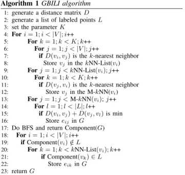
Algorithm 1 shows the steps to construct the graph G. Initially, it is necessary to generate a distance matrix D, Euclidean distance can be employed to generate it. In this matrix we can find theknearest neighbors of the elements. It is necessary to set the parameter K with a natural value and generate a list of the labeled points L.

In the algorithm, steps 5 to 8 find thek nearest neighbors for a vertexvi, then, steps 9 to 12 search for the mutualkNN

for vi and store them into a list. Steps 13 to 16 calculate the sum of the distances from vi to each element of the list

of mutual kNN and from these elements to a labeled point. It creates a connection between vi and vj that minimizes

this sum. Steps 17 to 22 post-process the graph connecting isolated components. It is important because mutual kNN graph, particularly for small values of k, often contain many disconnected components. These steps perform a Breadth-First Search (BFS) looking for components in the network. Compo-nents with no labeled point are connected with a neighboring

component with labeled point. We limit these new connections by a reduced number of links in order to avoid the network become too much dense.

Algorithm 1GBILI algorithm

1: generate a distance matrixD 2: generate a list of labeled pointsL 3: set the parameterK

4: Fori= 1;i <|V|;i++ 5: Fork= 1;k < K;k++ 6: Forj= 1;j <|V|;j++

7: ifD(vi, vj)is thek-nearest neighbor 8: Storevj in thekNN-List(vi) 9: Forj= 1;j < kNN-List(vi);j++ 10: Fork= 1;k < K;k++

11: ifD(vj, vi)is thek-nearest neighbor 12: Storevj in the M-kNN(vi) 13: Forj= 1;j <M-kNN(vi);j++ 14: Forl= 1;l <|L|;l++

15: ifD(vi, vj) +D(vj, vl)is min 16: Storeeij inG

17: Do BFS and return Component(G) 18: Fori= 1;i <|V|;i++ 19: ifComponent(vi)∈/L 20: Fork= 1;k < kNN-List(vi);k++ 21: ifComponent(vk)∈L 22: Storeeik inG 23: returnG

IV. COMPLEXITY ANALYSIS

Initially, it is necessary to compute a similarity among all pairs of nodes using a similarity function. This function generates a full adjacency matrix D ∈ n×n, where Dij =

d(vi, vj) is computed using Euclidean distance. To calculate

the Euclidean distance it takes n(n₂−1) steps, where n is the number of elements. Its complexity isO(n2).

Subsequently, we construct the graph. In this step the matrix D is sparsified and reweighted to produce the final matrixW. The sparsification is important because it improves the efficiency in the label inference stage. It generates a binary matrixP ∈Bn×n, wherePij = 1 indicates that there is an

edge between vi and vj, and Pij = 0 indicates the edge is

absent (assumePii= 0).

Based on the similarity matrix it is necessary to find the

k nearest neighbors of each element. For finding the kNN, the complexity isO(kn2), where nis the number of elements andkis the number of neighbors considered. But we need to calculate the mutualkNN, in this case, for eachjthneighbor of an element vi we need to check if vi ∈ kneighbors(vj).

For this reason, it takesk2nmore steps. The final complexity to find thek mutual neighbors isO(kn2+k2n). Ozaki et al. (2011) [16] use a Fibonacci heap-based implementation and construct the mutualkNN graph inO(n2+kn log n)time.

The proposed method creates a connection betweenviand

vjthat minimizes the sum of the distances fromvito its mutual

kNN and from this mutual kNN to a labeled point vl. For

each element, we need to access the similarity matrixkltimes, wherek is the mutual neighbors ofvi andl is the number of

labeled points. This cost is added with the cost of finding the

kNN mutual neighbor.

In the post-processing step it is necessary to find all components of the network, this can be done by Breadth-First Search (BFS). This algorithm begins at a root node and inspects all the neighboring nodes. For each node it inspects their neighbor nodes which were unvisited, and so on. Its time complexity isO(|V|+|E|) [7], where|V|is the number of vertices, and|E|is the number of edges. Since the constructed graph has average degree 2 (shown in Section V), by the equationk=2_VE, the number of edges is equal the number of vertices. When a component is identified, it is marked if it has or not a labeled point. If a vertexvibelongs to a component that have no labeled points, it will connect to one k nearest neighbors that belongs to a component with labeled point. In the worst case we need to look forkneighbors for npoints. Its complexity isO(kn).

Finally, the complexity of the proposed algorithm results inO(kn2+k2n+kln)+O(2n+kn), close tokNN method.

V. EXPERIMENTS

In this section we present extensive empirical results ex-ploring the GBILI method. Subsection V-A presents the de-scription of the data sets used and the setup of the experiments; subsection V-B shows the classification results; subsection V-C shows a parameter sensitivity analysis, a density analyzes of the graphs and theφ-Edge Ratio comparison betweenkNN and GBILI graphs. It is also provided the network visualization, which helps to understand the network topology; subsection V-D presents some centrality measures from Complex Net-works used to characterize GBILI network.

A. Data sets and experimental setup

The experiments were carried out on six data sets described in Table I. These data sets are frequently used in SSL literature and they were proposed by Chapelle et al. (2006) [6].

TABLE I. DATA SETS DESCRIPTIONS. Data set # Instances # Atrributes # Classes Comment

Digit1 1500 241 2 artificial and balanced g241c 1500 241 2 artificial and balanced g241n 1500 241 2 artificial and balanced

COIL2 1500 241 2 real and balanced

COIL6 1500 241 6 real and balanced

USPS 1500 241 2 real and imbalanced

First, we apply Principal Component Analysis (PCA) to all data sets reducing the dimensions to 50, because in high-dimensional data, the distance to the nearest neighbor ap-proaches the distance of the farthest neighbor, degenerating the quality of the graph. Then, we run experiments using 10 and 100 labeled vertices randomly selected from all the points. For the graph construction we apply kNN and GBILI methods. All such methods operate on the distance matrix

D∈ n×n, obtained from the Euclidean distance among the points. This process will result in a matrixPwherePij= 1if

a pointjhave a connection toiandPij= 0otherwise. Finally,

this matrix is symmetrized as followsPij=max(Pij,Pji). To

generate the weighted graphW we use the binary weighting approach (W = P). Some authors use the Gaussian kernel for weigh the graph. However, they do not have an agreement about which value apply in the kernel bandwidth parameterσ.

The algorithm used for the label inference task is Local and Global Consistency (LGC) [17], which is frequently used in the literature [11], [16]. LGC solves the optimization problem

F=argminF∈n×ctr(FTLF+μ(F−Y)T(F−Y)), which

gives the closed-form solution F = (I+L/μ)−1Y.I is the identity matrix,Y the set of known labels andLis the normal-ized Laplacian defined byL=D1/2LD1/2=I−D1/2WD1/2, whereDis the diagonal matrix with elementsDii=jWij.

Average classification accuracy of 30 runs is used as the evaluation measure.

Any other method based on graph can be applied for the label propagation task, for example, Gaussian Random Fields (GRS) [18], Laplacian Regularized Least Squares (Laplacian RLS) [1], etc. We compare the classification accuracy to the results presented by Chapelle et al. (2006) [6], for the fol-lowing algorithms: 1-NN, Discrete Reg., Transductive SVM, Cluster Kernel, Low-density separation (LDS), Laplacian RLS. It is worth pointing out that we use 10 and 100 labeled data randomly selected from all the points, while Chapelle et al. (2006) split the data into 12 partitions and select 10 and 100 labeled points from these partitions.

B. Classification results

In Tables II and III are the accuracy of the different methods for 10 and 100 labeled points for g241c, g241, digit1, COIL₆and USPS data sets.

TABLE II. AVERAGE ACCURACY WITH10LABELED POINTS. g241c g241n digit1 COIL6 USPS 1-NN 55.95 56.78 76.53 34.09 80.18 Discrete Reg. 50.41 50.95 87.36 36.62 83.93 TSVM 75.29 49.92 82.23 32.5 74.8 Cluster-Kernel 51.72 57.95 81.27 32.68 80.59 LDS 71.15 49.37 84.37 38.1 82.43 Laplacian RLS 56.05 54.32 94.56 45.46 81.01 kNN+LGC 55.16 51.69 89.61 41.59 83.54 GBILI+LGC 56.96 56.81 84.37 39.95 85.07

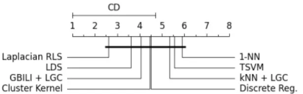
TABLE III. AVERAGE ACCURACY WITH100LABELED POINTS. g241c g241n digit1 COIL6 USPS 1-NN 59.72 62.51 93.88 76.73 92.36 Discrete Reg. 56.35 58.35 97.23 90.39 95.32 TSVM 81.54 77.58 93.85 74.2 90.23 Cluster-Kernel 86.51 95.05 96.21 78.01 90.32 LDS 81.96 76.26 96.54 86.28 95.04 Laplacian RLS 75.64 73.54 97.08 88.08 95.32 kNN+LGC 59.29 57.81 95.6 82.92 85.07 GBILI+LGC 61.77 66.95 95.6 82.92 94.1 We run the Nemenyi post-hoc test [8] to verify if it is possible to detect significant differences among algorithms from the results of the Tables II and III. According to the Ne-menyi statistics, the critical value for comparing the average-ranking of two different algorithms at 95 percentile is 3.50. The analysis is shown in Figure 2. The critical difference (CD) is on the top and the average ranks of measures are in the axis of the diagram. The lowest (best) ranks are in the left side, where we note that GBILI is better ranked than kNN. The methods analyzed have no significant difference, therefore they are connected by a black line in the diagram.

C. Parameter sensitivity and network density analysis Since we do not know a priori the optimal parameter k

to construct the graph, we test values ofkranging from 1to

Fig. 2. Comparison of all classifiers against each other with the Nemenyi test. Groups of classifiers that are not significantly different are connected.

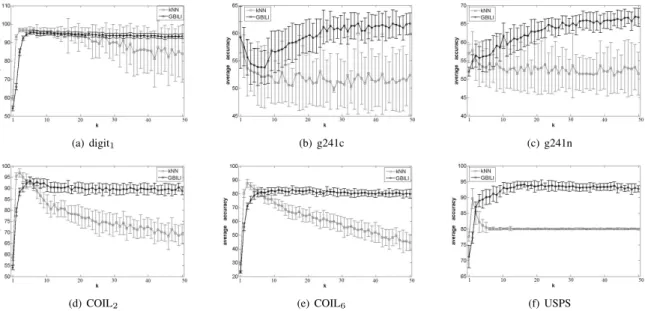
50to know how sensitive the graph generation methods are to this input parameter. Figure 3 shows the classification accuracy ofkNN and GBILI methods for 100 labeled examples. From these results we observe that kNN method usually leads to good results for values of k smaller than 10, because higher values of k turn the graph dense. In contrast, GBILI leads to better results for values of k bigger than 10, because it uses mutualkNN that finds less neighbors thankNN method, so it is necessary a higher value of k to have more mutual neighbors. In GBILI graphs, we observe the classification accuracy stabilizes after k > 10, indicating we could use a fixed value of kbigger than10.

Figure 4 shows the comparison of average degree among

kNN, mutualkNN and GBILI. Just GBILI is not affected byk

and achieves a constant number of edges, presenting an average degree around 2, independent of the k. Hence, the proposed method generates sparser graphs thankNN.

Fig. 4. Average degree in akNN, mutualkNN and GBILI graphs built using the USPS data set.

Figure 5 shows the graphs generated bykNN and GBILI methods for USPS data set with 10 labeled points. We set the value of k according to the high accuracy achieved by the methods. HencekNN useskequal 3 and generates a network with average degree around 4.5 and GBILI uses akequal 30 and generates a network with average degree around 2. The quantity of edges in a network is related with the processing cost and efficiency of the SSL algorithms, so it is interesting have sparser graphs.

The density affects the methods classification accuracy as we can see by comparing theφ-edge ratios ofkNN and GBILI methods. We utilizeφ-edge ratioas Ozaki et al. (2011) [16] to measure the quality of a graph. These authors defineφ-edgeof a labeled graph (G,y) as any edge (vi, vj) for whichyi=yj,

andφ-edge ratioof a graph as the number ofφ-edge divided by the total number of edges in the graph.

Since most graph-based SSL classification methods

(a) digit1 (b) g241c (c) g241n

(d) COIL2 (e) COIL6 (f) USPS

Fig. 3. Average accuracy rates and standart deviations comparisons for (a)digit1, (b)g241c, (c)g241n, (d)COIL2, (e)COIL6and (f)USPS data sets using 100 labeled examples.

Fig. 5. kNN and GBILI graphs for USPS data set using 10 labeled examples.

gate label information throw the network, edges connecting vertices with different labels may lead to misclassification. Hence, a graph with a smallerφ-edge ratio is better.

Figure 6 shows the plots of φ-edge ratios of GBILI and

kNN methods for COIL₂and USPS data sets. We notice that the same pattern occurs for all data sets. The y-axe denotes the

φ-edge ratio of the constructed graphs and the x-axe denotes the parameter k used. But the number of edges is different in the resulting graphs for these methods: as the value ofk

increases, the number of edges inkNN increases too, but in GBILI the number of edges is always the same. This way,kNN method achieves higherφ-edge ratio than GBILI and a worst classification accuracy when the value ofkbecomes higher.

D. Complex networks measures

GBILI method generates hubs from the labeled points (black nodes in Figure 5). This network approximates to an “exponential network” since the probability of finding a node with connectivity (or degree) k different from the

Fig. 6. Averageφ-edge comparisons for COIL2(left) and USPS (right) data sets using 10 labeled examples withkNN and GBILI graph construction. The smaller theφ-edge ratio, the better the graph.

average connectivity decays exponentially fast for largek. We explore centrality measures from the GBILI network and we demonstrate that labeled vertices are important in the network topology. The measures explored arenode degree,betweenness [10],eigenvector centrality [3] andpageRank[4].

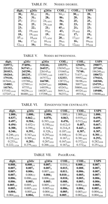
These measures are presented in Tables: IV (node degree), V (betweenness), VI (eigenvetor) and VII (pageRank) for digit₁, g241c, g241n, COIL₂, COIL₆and USPS data sets with 10 labeled points. We present the 10 highest values from the GBILI networks. The vertices numerate from 1 to 10 are labeled and their measures are shown in bold in the tables. The subscript is the number of the vertex.

In real networks the presence of nodes with a very large number of connections (hubs) facilitates spreading information or epidemics, especially if the hubs are infected. The GBILI algorithm generate hubs from the labeled points, as we can see in Table IV, where most of the labeled points have the biggest degree in the network. In Table V many labeled points have high betweenness, so they belong to many geodesic paths. It means these points influence many nodes in the network and are important to transmit information throw the network. Furthermore, a vertex is important also when it receives connections from important vertices. Such relevance is

indicated by Eingenvector centrality and PageRank, see Tables VI and VII, respectively.

The network topology is related to information propagation on Complex Networks. GBILI method construct networks exploring the labeled vertices and these points can become hubs. The centrality measures, calculated here, indicate these vertices are important in the network, in this way, GBILI topology can facilitate the label propagation task.

TABLE IV. NODES DEGREE. digit1 g241c g241n COIL2 COIL6 USPS

302 3210 316 9417 3010 281 296 319 288 865 281 266 277 2577 241491 569 255 254 263 253 241348 501 239 257 235 224 212 4510 218 235 221 191060 1920 434 21402 212 184 191205 191 4050 173 198 1710 18468 171456 2811 17257 1910 169 1732 16192 2665 164 16936 12612 168 16769 2538 12682 14398

TABLE V. NODES BETWEENNESS.

digit1 g241c g241n COIL2 COIL6 USPS

3209722 3740969 3182446 2353755 1294598 2900771 2311526 36374310 2645278 156545337 76138130 2571685 2010535 2452903 22614520 15166536 717485 186240581 1842643 2012354 1753951348 14007517 714371142 1806727 1791109 1405625 16757263 1323531 59952286 1794144 167644133 13578832 1667801 12872392 58196379 1603606 1548811 12799177 162047631 1020448 50977658 15475910 1417614 9775323 14935933 6524391 508041069 149967398 1371021040 94256113 1402871491 56913144 49324189 1494088 127247114 884801205 137298410 5623370 4931424 138086983

TABLE VI. EINGENVECTOR CENTRALITY.

digit1 g241c g241n COIL2 COIL6 USPS

1.0002 1.0009 1.0006 1.00017 1.000402 1.0001 0.8376 0.86210 0.8708 0.8635 0.919257 0.6996 0.4973 0.5843 0.3931348 0.4709 0.512682 0.6874 0.4947 0.45277 0.350234 0.41250 0.4879 0.6675 0.3885 0.39932 0.34366 0.21438 0.44310 0.6097 0.3461 0.3914 0.32814 0.187158 0.3875 0.3072 0.2461275 0.343468 0.293969 0.168218 0.381403 0.30110 0.2351219 0.305461 0.29146 0.16715 0.381495 0.2938 0.23334 0.2815 0.267232 0.167929 0.372219 0.282398 0.2221158 0.2791063 0.2661456 0.16790 0.37236 0.251823

TABLE VII. PAGERANK.

digit1 g241c g241n COIL2 COIL6 USPS

0.0082 0.00810 0.0076 0.01617 0.00810 0.0071 0.0076 0.0079 0.0078 0.0155 0.0081 0.0076 0.0077 0.0063 0.0071491 0.0111 0.0065 0.0074 0.0073 0.00677 0.0062 0.01010 0.0058 0.0077 0.0065 0.0061060 0.0061348 0.0109 0.0059 0.0062 0.0061 0.0054 0.0051 0.0084 0.0053 0.0065 0.00510 0.0051205 0.0051456 0.00750 0.004402 0.0058 0.0054 0.0051450 0.005769 0.0068 0.0044 0.00510 0.0049 0.005468 0.004192 0.0052 0.003257 0.004936 0.0041002 0.0048 0.00420 0.00511 0.002809 0.004398 VI. CONCLUSION

In this paper we explore how labeled instances, available in the SSL setting, can be used to construct a better graph for classification in SSL. We provide extensive empirical evidence that this technique called GBILI leads to good classification accuracy. Furthermore, we provide a detailed complexity analys in which we show GBILI has the same time complextiy of kNN graphs. We show that kNN gen-erates more dense networks than GBILI and by using the

φ-edge ratio measure we confirm that when the parameter

k increases, the quantity of edges connecting vertices with different labels increases too, propagating wrong information. We also apply centrality measures from Complex Network to characterize GBILI networks. The exploited measures were node degree, betweenness, eigenvector and pageRank. These measures confirm the labeled points in GBILI graph are hubs and important in network topology. So, they can facilitate the label propagation process.

ACKNOWLEDGMENT

Grant 2011/21880-3 and 2011/22749-8 Sao Paulo Research Foundation (FAPESP).

REFERENCES

[1] Belkin, M.; Niyogi, P.; Sindhwani, V. (2006)Manifold regularization: A geometric framework for learning from labeled and unlabeled examples. Journal of Machine Learning Research, v. 7, p. 2399-2434.

[2] Berton, L.; Lopes, A. A. (2012)Informativity-based graph: exploring mutual kNN and labeled vertices for semi-supervised learning. In 4th International Conference on Computational Aspects of Social Networks, p. 14-19.

[3] Bonacich, P. (1972) Factoring and weighting approaches to clique identification. Journal of Mathematical Sociology, v. 2, p. 113-120. [4] Brin, S.; Page, L. (1998)The anatomy of a large-scale hypertextual web

search engine. Computer Networks and ISDN Systems, p. 107-117. [5] Brito, M. R.; Chavez, E. L.; Quiroz, A. J.; Yukich, J. E. (1997)

Connectivity of the mutual k nearest neighbor graph in clustering and outlier detection. Statistics and Probability Letters, v. 35, p. 33-42. [6] Chapelle, O.; Schlkopf, B.; Zien, A. editors (2006) Semi-Supervised

Learning. MIT Press, Cambridge, MA.

[7] Cormen, T. H.; Leiserson, C. E.; Rivest, R. L.; Stein, C. (2009) Introduction to Algorithms. MIT Press and McGraw-Hill, 3rd ed. [8] Demsar, J. (2006)Statistical Comparisons of Classifiers over Multiple

Data Sets. Journal of Machine Learning Research, v. 7, p. 1-30. [9] Dhillon, P. S.; Talukdar, P. P.; Crammer, K. (2010) Inference Driven

Metric Learning (IDML) for Graph Construction. Technical Reports (CIS), University of Pennsylvania.

[10] Freeman, L. C. ( 1977) A set of measures of centrality based on betweenness. Sociometry, v. 40, p. 35-41.

[11] Jebara, T.; Wang, J.; Chang, S.F. (2009) Graph construction and b-matching for semi-supervised learning. In Proceedings of the 26th Annual International Conference on Machine Learning, p. 441-448. [12] Maier, M.; Hein, M.; Luxburg, U. (2007) Cluster Identification in

Nearest-Neighbor Graphs. In Proceedings of the 18th international conference on Algorithmic Learning Theory, p. 196-210.

[13] Maier, M.; Luxburg, U. (2009) Influence of graph construction on graph-based clustering measures. The Neural Information Processing Systems, v. 22, p. 1025-1032.

[14] Rohban M. H.; Rabiee, H. R. (2012).Supervised neighborhood graph construction for semi-supervised classification. Pattern Recognition, v. 45, p. 1363-1372.

[15] Newman, M. (2003)The structure and function of complex networks. SIAM Review, v. 45, p. 167-256.

[16] Ozaki, K.; Shimbo, M.; Komachi, M.; Matsumoto, Y. (2011)Using the Mutual k-Nearest Neighbor Graphs for Semi-supervised Classification of Natural Language Data. In Proceedings of the 15th Conference on Computational Natural Language Learning, p. 154-162.

[17] Zhou, D.; Bousquet, O.; Lal, T. N.; Weston, J.; Schlkopf, B. (2004) Learning with local and global consistency. In Advances in Neural Information Processing Systems, v. 16, p. 321-328: MIT Press. [18] Zhu, X.; Ghahramani, Z.; Lafferty, J. (2003)Semi-supervised learning

using Gaussian fields and harmonic functions. In Proceedings of the Twentieth International Conference on Machine Learning, p. 912-919. [19] Zhu, X. (2005)Semi-supervised learning literature survey. Technical

report 1530 - Computer Sciences, University of Wisconsin-Madison.