Randomizing Dispatch Scheduling Policies
Vincent A. Cicirello
and
Stephen F. Smith
The Robotics Institute Carnegie Mellon University
5000 Forbes Avenue Pittsburgh, PA 15213
fcicirello, [email protected]
Abstract
The factory is a complex dynamic environment and schedul-ing operations for such an environment is a challengschedul-ing prob-lem. In practice, dispatch scheduling policies are commonly employed, as they offer an efficient and robust solution. How-ever, dispatch scheduling policies are generally myopic, and as such they are susceptible to sub-optimal decision-making. In this paper, we attempt to improve upon results of such dispatch policies by introducing non-determinism into the decision-making process, and instead using a given policy as a baseline for biasing stochastic decisions. We consider the problem of weighted tardiness scheduling with sequence-dependent setups with unknown arrival times in a dynamic environment, and show that randomization of state-of-the-art dispatch heuristics for this problem in this manner can im-prove performance. Furthermore, wefind that the “easier” the problem, the less benefit there is from randomization; the “harder” the problem, the more benefit. Our method of ran-domization is based on a model of the way colonies of wasps self-organize social hierarchies in nature.
Introduction
In dynamic factory environments, dispatch scheduling poli-cies provide a practical, robust basis for managing execu-tion. Scheduling decisions are made in an online manner only when needed, based on the current state of the factory. Dispatch policies make use of information about jobs such as expected processing time, setup time, due date, priority, etc., and are typically designed to optimize a given perfor-mance objective. Their virtue is their simplicity and insensi-tivity to environmental dynamics and for these reasons they are commonly employed. At the same time, the localized and myopic nature by which decisions are made under such schemes make them inherently susceptible to sub-optimal decision-making. (see (Morton & Pentico 1993) for a thor-ough review of dispatch scheduling).
In this paper, we explore the idea of randomizing dis-patch policies to improve their performance. We start from the perspective that a given dispatch policy provides a good decision-making baseline, but it is not infallible and will sometimes make suboptimal choices. Hence, instead of un-conditionally following its decisions, we use the dispatch policy to bias a stochastic selection process. Randomizing heuristics to improve decision-making performance is not a
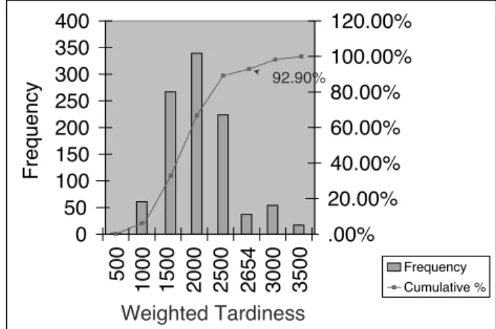
0 50 100 150 200 250 300 350 400 500 1000 1500 2000 2500 2654 3000 3500 .00% 20.00% 40.00% 60.00% 80.00% 100.00% 120.00% Frequency Cumulative % Weighted Tardiness Frequency 92.90%
Figure 1: This histogram partitions 1000 trials of a random-ized version of the dispatch policy COVERT on an instance of a weighted tardiness problem with sequence-dependent setups. Each bucket contains the trials with results in a given range of the weighted tardiness objective. COVERT pro-duces a solution with weighted tardiness of 2654 for this instance. 92.9% of the random trials gave better solutions.
new idea; but to our knowledge this is thefirst attempt to do so in an online control setting.
Our approach hypothesizes that solution obtained using a dispatch policy is surrounded by a neighborhood of po-tentially “better” solutions. This hypothesis is based on a couple of observations. First, dispatch policies in practice tend to be quite sensitive to parameter settings and in fact they are frequently tuned to individual problem instances in experimental studies. (Such tuning is of course not possi-ble in online settings.) Second, dispatch policies are of-ten designed for idealized problems as they are adapted to accommodate more complex constraints this can result in more imprecise state estimation. Figure 1 shows the results of 1000 trials of a randomized dispatch policy designed to minimize weighted tardiness, partitioned according to ob-served weighted tardiness. Of these trials, 92.9% produced results better than the deterministic policy, giving empirical evidence of the potential of randomization.
We focus specifically on a weighted tardiness scheduling
problem with sequence dependent setups. In our problem, jobs arrive dynamically with specific due dates and priori-ties, and the goal is to minimize average weighted tardiness. The problem is further complicated by the fact that the ma-chines used to process jobs, though they are multi-purpose, require some nontrivial amount of setup time to change-over from processing a job of one type to processing a job of an-other type.
Two of the best regarded dispatch policies for the weighted tardiness problem are COVERT (Vepsalainen & Morton 1987) and R&M (Rachamadugu & Morton 1982). Both are considered state-of-the-art (Morton & Pentico 1993); but neither were actually designed with sequence-dependent setups in mind. In fact, we are aware of only two reported dispatch heuristics for weighted tardi-ness scheduling under sequence-dependent setups (Raman, Rachamadugu, & Talbot 1989; Lee, Bhaskaran, & Pinedo 1997), both of which are derived by making (slightly differ-ent) modifications to the R&M dispatch policy to account for setup time.
In the remainder of this paper, wefirst review prior work in heuristic-biased stochastic scheduling methods. We then describe our approach of randomizing dispatch scheduling policies based on a model of wasp behavior. The paper then continues with a discussion of experimental results and con-clusion.
Heuristic-Biased Search
Heuristic-biased random strategies have been used as effec-tive iteraeffec-tive search strategies in a number of scheduling-related contexts. In (Watsonet al.1999), Watson et al. study the effects of problem structure on a number of scheduling algorithms for theflow-shop problem. They argue that more complex algorithms which work well on randomly gener-ated benchmark problems often fail to live up to expecta-tions when applied to real problems. The problem from their point of view is that real problems often contain structure of one sort or another that is not present in randomly gener-ated benchmark problems. They hypothesize that more com-plex, carefully crafted algorithms can become over-tuned to the benchmarks. In their study, they compare a number of scheduling approaches for the flow-shop scheduling prob-lem and show that as real-world probprob-lem-inspired structure is added to the problem, the faster and simpler stochastic al-gorithms are superior to the more complex “state-of-the-art” deterministic algorithms.
In (Bresina 1996), Bresina introduced a random restart search technique called heuristic-biased stochastic sampling (HBSS). HBSS performs a random search biased accord-ing to a heuristic for the problem. Bresina considered the scheduling of observations on a telescope. His approach be-gan by ordering the observations according to a heuristic and giving each a rank according to the resulting order. The next observation would then be selected by a random process bi-ased according to a function of these rankings. Different bias functions lead to more or less biasing in favor of the heuris-tic. So the choice of bias function depends on confidence in the heuristic.
Oddi and Smith (Oddi & Smith 1997) explored a related idea as the basis for solving a generalized job shop schedul-ing problem. One important distinction in this approach is acknowledgement of the fact that a heuristic may be more or less informed in different decision-making contexts, and hence the degree of confidence in the heuristic can vary from decision to decision. Rather than rely on a static bias function as is used in HBSS, Oddi and Smith define non-deterministic variants of search control heuristics that vary the degree of randomness as a function of how informed the heuristic is. A variant of this idea is also exploited by Cesta et al. (Cesta, Oddi, & Smith 2001) in solving a resource-constrained project scheduling problem.
In this paper, we take a similar approach but our goal is to make more effective control decisions rather than to broaden a search process. We bias our random decisions not by a function of a ranking given by the dispatch policy, but rather by a function of the value of the dispatch heuristic itself. In a control setting, it is particularly important to calibrate the degree of randomness of a decision to some measure of how discriminating the dispatch heuristic is in this decision context. Since we are making online decisions, we want nondeterminism when chances of finding a better solution than that proposed by the heuristic are best.
Scheduling Wasps
Our approach to randomization derives from a naturally-inspired computational model of the self-organization that takes place within a colony of wasps. (Theraulazet al.1991; Theraulaz, Bonabeau, & Deneubourg 1995; Bonabeau et al. 1997). In nature, a hierarchical social order among the wasps of the colony is formed through interactions among individual wasps of the colony. This emergent social order is a succession of wasps from the most dominant to the least dominant (analogous to a prioritization of jobs on a set of machines). In the model of Theraulaz et al., the results of these interactions are determined stochastically based on the “force” variables of the wasps involved. The probability of wasp 1 winning a dominance contest against wasp 2 is
de-fined based on the force variables, F
1and F 2, of the wasps as: P
(
F 1 F 2) =
F 2 1 F 2 1+
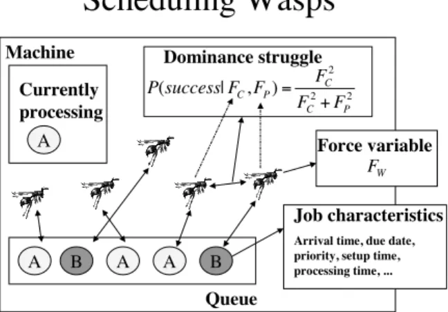
F 2 2 (1) This model can be directed mapped to the problem of prioritizing jobs in a queue, and as such provides a natu-ral basis for the randomization of dispatch policies. In our “scheduling wasp” formulation, each job is represented by a wasp and the concept of a force variable is used to de-fine job priority (i.e., the value that the dispatch policy in use assigns). The scheduling wasps then interact with each other to prioritize the jobs in the queue. This framework for dynamic scheduling wasfirst introduced in (Cicirello & Smith 2001), where we considered the problem of sequenc-ing jobs to maximize throughput under different and dynam-ically changing job mixes. Here we explore the use of this wasp model on due date problems, where dispatch-based so-lutions are more commonly employed.Scheduling Wasps
Machine Queue A B A A B A Currently processing Force variable Job characteristics Arrival time, due date, priority, setup time, processing time, ... Dominance struggle 2 2 2 ) , | ( P C C P C F F F F F success P + = W FFigure 2: Scheduling wasps
To fully specify our scheduling wasp model for mini-mizing weighted tardiness with sequence dependent setups, we need to provide a definition of force. We will consider two alternatives: 1) COVERT (Vepsalainen & Morton 1987) and 2) R&M (Rachamadugu & Morton 1982). As men-tioned earlier, neither of these dispatch policies was origi-nally designed with sequence-dependent setups in mind. We have here modified both COVERT and R&M to account for setup time. The modification of R&M was made previously in (Raman, Rachamadugu, & Talbot 1989) and we have here made the equivalent modification to COVERT.
Noting this, the two alternative definitions of force are: 1. COVERT:F w
=
Ww T p w+T s w(1
:0
; (Dw;T p w ;T s w ;Tnow) + h(T p w+T s w ))
+ 2. R&M:F w=
W w T p w +T s wexp(
;(D w ;T p w ;T s w ;Tnow) + hT p)
whereT p wand T sware the processing time and setup time of
waspw’s job,D
wis the duedate, W
wis the weight, Tnow
is the current time,T p
is the average processing time, and
(
A)
+
= max
fA
0
g. The winner of a dominance contest inthis context is determined stochastically in the same manner as in the model of real wasp behavior.
Dominance Tournaments
We have so far left open the question of what actually hap-pens when a machine becomes available. In the typical dis-patch scheduling approach, the job in the queue with the highest value of the dispatch heuristic is chosen next. Given the scheduling wasp formulation of the previous section, our system instead chooses the next job based on a tournament of dominance contests. We consider four dominance tourna-ments which form a progression from the most randomized to the least randomized. These four tournaments are: 1. Step-Ladder (W-V1): In this tournament, the scheduling
wasps are seeded based on their current position in the queue. The last two wasps in the queue engage in a dom-inance contest. The winner then engages in a domdom-inance contest with the next wasp and so forth along the length of the queue. As this occurs, the jobs associated with
the winning wasps move closer to the front of the queue. Whatever job is at the front of the queue when this process completes is chosen next by the machine.
2. Single-Elimination (W-V2): In this tournament, the scheduling wasps are seeded arbitrarily and take part in a single-elimination tournament. At each level of the tour-nament exactly half of the wasps are eliminated. This style tournament is biased slightly more in favor of what-ever dispatch heuristic is used as force when compared to the previous. In W-V1, a job with a low force value at the front of the queue can potentially get lucky and win its only dominance contest; whereas in W-V2 winning a single dominance contest is not sufficient (unless there are only two jobs in the queue).
3. Double-Elimination (W-V3): This tournament is one step less random then the previous. Again the wasps are seeded arbitrarily. But this time, two simultaneous tourna-ments alternate rounds. That is, the primary tournament consists of undefeated wasps. The losers at each round move to the secondary tournament. In the secondary tour-nament, losers are eliminated. The winner of the primary tournament then gets two chances (has not lost yet) of eliminating the winner of the secondary tournament. If it is unsuccessful in both attempts then the winner of the secondary tournament is chosen by the machine. In this way, a wasp with a high force value that was unlucky and lost early in the tournament still has a chance of winning. 4. One-More-Chance (W-V4): This method begins by con-ducting a double-elimination tournament as in W-V3. If the winner also happens to have the highest value of the dispatch heuristic then it is chosen. Otherwise, it engages
in afinal dominance contest with the wasp with the
high-est value. And the winner of this dominance conthigh-est is taken next by the machine. So as you can see this is yet another step in the less random direction.
Degrees of Randomness
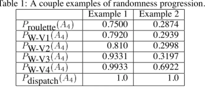
In describing the dominance tournaments above, we stated that the four models form a progression along a random-ness scale beginning with the most random (W-V1) and end-ing with the least random (W-V4). Deterministic dispatch scheduling can be seen as a last step in this progression. To illustrate this progression, consider two examples. In Exam-ple 1 there are 4 jobs in the queue: A
1 A 2 A 3 A 4. Now
consider that we have a dispatch heuristic H that assigns
the following values to these jobs: H
(
A 1) =
H(
A 2) =
H(
A 3) = 1
and H(
A4
) = 3
. Let the ForceF be defined
by this heuristic. In Example 2, everything is the same ex-cept thatH
(
A4
) = 1
:
1
. In Table 1 we list the probabilitythat jobA
4is chosen next by the machine in each example
for each of the defined dispatching methods. In addition to showing the progressive increase in randomness through the wasp tournament variations, this Table illustrates the desired general property that the more certain the dispatch heuristic is, the less random the decision produced by our randomiza-tion methods; and the less certain the dispatch heuristic is the more random the decision.
Table 1: A couple examples of randomness progression. Example 1 Example 2 P roulette
(
A 4)
0.7500 0.2874 P W-V1(
A 4)
0.7920 0.2939 P W-V2(
A 4)
0.810 0.2998 P W-V3(
A 4)
0.9331 0.3197 P W-V4(
A 4)
0.9933 0.6922 P dispatch(
A 4)
1.0 1.0Experimental Design
All of the experiments that are presented here were per-formed in a simulated factory environment implemented in Java and executed on a Pentium III running Linux 5.2. We consider factories that produce two products (henceforth, Job Type A and Job Type B) as well as three products (Job Type A, Job Type B, and Job Type C). All machines in the factory are multi-purpose machines that can process any of these types (only single stage jobs are considered here). Ex-periments with one, two, and four machines are studied. In all cases, setup time to reconfigure a machine for a different job type is 30 time units.
In the two job type experiments, jobs are released to the factoryfloor dynamically according to three different prod-uct mixes. In each, arrival rates are defined by the proba-bility a new job of each type is released during a given time unit. The arrival rates for the one machine problems are as follows:
50/50 mix: P(Job Type A) = 0.025, P(Job Type B) = 0.025 85/15 mix: P(Job Type A) = 0.04285, P(Job Type B) =
0.00715
100/0 mix: P(Job Type A) = 0.0665, P(Job Type B) = 0.0
Multiply these rates by 2 to get the arrival rates for the two machine problems and by 4 to get the rates for the four ma-chine problems.
In the three job type experiments, the arrival rates are de-fined similarly for the one machine problem (make the same appropriate adjustments as above for two and four machine problems):
33/33/33 mix: P(Job Type A) = 0.0166, P(Job Type B) =
0.0166, P(Job Type C) = 0.0166
50/25/25 mix: P(Job Type A) = 0.025, P(Job Type B) =
0.0125, P(Job Type C) = 0.0125
These arrival rates correspond approximately to medium-to-heavily loaded factories.
When a new job is generated, its process time is 15 plus a Gaussian noise factor, its weight is drawn uniformly from the interval
1
20]
, and its duedate is drawn uniformly fromone of the following intervals (where P is process time, W is weight, and T is current time):
TT
+ 4
P]
ifW >16
TT+ 6
P]
if12
<W16
TT+ 6
:5
P]
if8
<W12
TT+ 8
P]
ifW8
Two sets of experiments were performed. The first us-ing COVERT as the definition of the force variable for the scheduling wasps (the second using R&M). In each set of experiments, the four variations of the scheduling wasp selection method were compared to the base determinis-tic dispatch heurisdeterminis-tic. For each combination of schedul-ing method and job mix, 100 simulations with different ar-rival sequences were performed and each simulation was at least 1000 time units in length (jobs stop arriving at time unit 1000 and simulation ends when all jobs have been pro-cessed).
Experimental Results
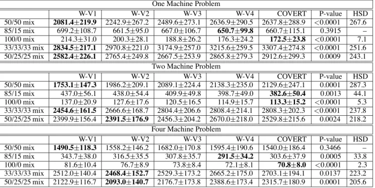
In Table 2 we see the average weighted tardiness of 100 sim-ulations for the one, two, and four machine problems with two and three job types for various job mixes. The results in this table compare the variations of the scheduling wasps (using COVERT as force) with that of the dispatch heuristic COVERT. You willfirst notice that for the 100/0 job mix and for each of one, two, and four machines that COVERT per-forms best. The result is statistically significant according to an ANOVA with correlated samples. This is to be expected. The 100/0 mix is a single job type problem and therefore sequence-dependent setups are not an issue. This is what COVERT was especially designed for (i.e., no setups) so randomizing is almost certain to give us worse results. But do note that as you scan across the rows corresponding to the 100/0 job mix that the less random the scheduling wasp se-lection method, the closer the results are to that of COVERT. In fact, the result of a Tukey HSD test show in all cases no significance between W-V4 and COVERT.
Now turn your attention to the 85/15 job mix. This case is slightly less like a one job type problem and the sequence-dependent setups may play an active part. In the one, two, and four machine problems, the best results are again to-ward the COVERT end of the chart with W-V4 edging out COVERT slightly in all but the two machine problem. How-ever, the one machine result is not statistically significant and in both the two and four machine case the pairwise re-sult of W-V4 and COVERT is not significant according to the Tukey HSD test.
Next, examine the 50/50 job mix results. In this case, min-imization of setups is much more crucial to performance. And in every case, we see that the most random of the wasp variations (WV-1) performs best and in all but the four ma-chine problem the result is statistically significant. In the four machine problem, there are more degrees of freedom for the system to work with. That is, if a machine M1 is mislead by COVERT into taking a particular job J1 when J2 would have been better, there are three other machines M2, M3, and M4 that mayfinish whatever they are doing in time to pick up job J2 before it sits around long enough to cause any serious harm to the objective. In a sense the four machine problem is “easier” than the one and two machine problems and randomization seems to buy us less.
Based on the two job type problems using COVERT, it appears that the trend is that the more sequence-dependent setups are a factor to the problem, then the greater the ben-efit of randomization. And alternatively, the less
sequence-Table 2: Average weighted tardiness for different job mixes. COVERT is used as the Force definition for all variations of the scheduling wasp approach. The results are compared to COVERT. 95% confidence intervals and P-values from ANOVA tests with correlated samples are shown. HSD is the absolute difference between any two means required for significance at the 0.05 level according to the Tukey HSD test.
One Machine Problem
W-V1 W-V2 W-V3 W-V4 COVERT P-value HSD 50/50 mix 2081.4219.9 2242.9267.2 2489.6273.1 2636.9290.5 2637.8288.9 <0.0001 267.6 85/15 mix 699.2108.7 661.595.0 667.0106.7 650.799.8 660.7115.1 0.3915 – 100/0 mix 214.331.0 200.328.1 188.826.2 176.324.2 172.523.8 <0.0001 7.1 33/33/33 mix 2834.5217.1 2970.8221.0 3174.9257.0 3215.6259.5 3307.4274.8 <0.0001 251.6 50/25/25 mix 2582.4226.1 2765.4249.8 2667.5253.9 2865.8279.3 2912.6299.3 0.0009 243.1
Two Machine Problem
W-V1 W-V2 W-V3 W-V4 COVERT P-value HSD 50/50 mix 1753.1147.3 1986.2209.1 2089.1224.4 2138.3235.0 2129.6247.1 0.0001 287.3 85/15 mix 437.056.1 438.054.4 409.949.8 398.749.0 382.650.4 0.0013 44.1 100/0 mix 137.020.9 127.617.6 120.516.5 114.915.7 113.315.2 <0.0001 5.3 33/33/33 mix 2454.6161.5 2666.6168.7 2804.4206.6 2808.4214.1 2808.3202.3 <0.0001 237.8 50/25/25 mix 2399.9156.4 2391.5176.9 2456.3204.2 2670.0218.0 2529.8215.6 0.0024 218.2
Four Machine Problem
W-V1 W-V2 W-V3 W-V4 COVERT P-value HSD 50/50 mix 1490.5118.3 1558.2146.2 1682.0170.8 1595.4190.6 1540.0186.4 0.3466 – 85/15 mix 343.738.0 316.535.5 307.835.7 291.534.2 303.637.9 0.0005 33.8 100/0 mix 81.610.4 76.78.9 73.88.4 72.18.1 70.88.0 <0.0001 2.3 33/33/33 mix 2512.0140.4 2468.4152.7 2529.3173.2 2665.2175.0 2703.1194.1 0.0137 223.2 50/25/25 mix 2122.9116.7 2093.0140.7 2176.7173.8 2388.6173.4 2315.7180.9 0.0001 205.6
dependent setups are an issue the less randomized the heuris-tic should be. Also the more difficult the problem then the more randomization is needed.
We now turn to the results of the three job type problems (also appearing in Table 2) to see if this hypothesis holds. In both the 33/33/33 and 50/25/25 job mix problems, sequence-dependence should be more of an issue than the two job type problems and thus the problems should be more difficult. All results for both of the three job type mixes are statistically significant according to an ANOVA with correlated samples. Also for all numbers of machines and for all three job type mixes, the best result is either W-V1 or W-V2 (the more random end of the chart) with no significance between the W-V1 and W-V2 results according to Tukey HSD tests.
In Table 3 we see the complimentary results using R&M as the force value for the wasps as compared directly to using the dispatch heuristic R&M. In all cases there is no significant difference in the performance of R&M as com-pared to COVERT (from the previously discussed results) and there is also no significant difference between the best of the scheduling wasp variations using either dispatch heuris-tic as force. The overall trends seem to show the same thing as well. The more difficult the problem and the more that sequence-dependent setups are an issue, the more to be gained by randomization. The “easier” the problem, the bet-ter off is non-randomized dispatch scheduling.
Weighted Roulette Wheel
We have advocated our wasp model as a basis for random-ization of dispatch policies. It is natural to ask whether or not there is a simpler way to randomize dispatch schedul-ing policies. One possibility that we consider is borrowed from the evolutionary computation community. The genetic algorithm (GA) selection strategy known asfitness propor-tional selection allocates to each individual of the population a chunk of a roulette wheel in size proportional to itsfitness relative to the rest of the population. In a GA, this weighted roulette wheel would be spunntimes to choose then
mem-bers of the successive generation.
As an alternative to our wasp formulations, we use a weighted roulette wheel. Each jobjin the queue is allocated
a portion of the wheel proportional to the square of its force value (i.e.,F
2
j). And when a machine becomes available this
wheel is spun once to select the next job from the queue. You can think of this as a generalization of a dominance contest between two wasps to that of a sort of “free-for-all” among all of the wasps in the nest. In this case, the probability that jobjis processed by the available machine is given by:
P
(
F j) =
F 2 j P n k =1 F 2 k (2) In Table 4, we see a comparison among W-V1 (using COVERT as Force), COVERT, and the weighted roulette wheel approach (Roulette) just described. We have chosen W-V1 for this comparison because it is the best performer overall from among the wasp variations. We can use this asTable 3: Average weighted tardiness for different job mixes. R&M is used as the Force definition for all variations of the scheduling wasp approach. The results are compared to R&M. 95% confidence intervals and P-values from ANOVA tests with correlated samples are shown. HSD is the absolute difference between any two means required for significance at the 0.05 level according to the Tukey HSD test.
One Machine Problem
W-V1 W-V2 W-V3 W-V4 R&M P-value HSD 50/50 mix 2133.5234.2 2307.1267.4 2372.3250.0 2737.8298.1 2636.6295.4 <0.0001 258.8 85/15 mix 691.6110.6 678.298.6 666.6100.9 656.9104.8 665.5116.0 0.7284 – 100/0 mix 215.831.2 204.528.6 190.526.0 178.924.5 175.424.1 <0.0001 7.2 33/33/33 mix 2835.1202.6 3013.9235.3 3132.7251.6 3220.6264.9 3325.2272.4 <0.0001 260.1 50/25/25 mix 2581.0223.0 2785.8251.6 2711.0256.3 2887.3281.4 2917.2296.1 0.0011 245.9
Two Machine Problem
W-V1 W-V2 W-V3 W-V4 R&M P-value HSD 50/50 mix 1660.0151.5 1979.3209.1 2083.5206.6 2118.0230.3 2111.0240.1 <0.0001 281.7 85/15 mix 446.155.4 429.550.4 419.453.6 393.853.2 386.450.0 0.0009 44.3 100/0 mix 139.721.1 130.817.8 122.716.4 116.215.5 115.315.3 <0.0001 5.4 33/33/33 mix 2554.5168.7 2611.0155.0 2674.6209.2 2890.7211.2 2760.8199.5 0.0014 240.9 50/25/25 mix 2375.7168.7 2409.7183.0 2449.1193.1 2645.0215.1 2563.9222.4 0.0035 219.1
Four Machine Problem
W-V1 W-V2 W-V3 W-V4 R&M P-value HSD 50/50 mix 1513.5125.2 1518.0159.6 1677.1195.4 1559.7173.5 1540.9191.2 0.4074 – 85/15 mix 344.240.2 309.133.5 305.934.4 296.833.9 300.737.8 0.0010 34.0 100/0 mix 83.510.4 79.28.9 75.68.4 73.88.1 73.38.1 <0.0001 2.2 33/33/33 mix 2457.1134.2 2534.1161.0 2598.1182.6 2684.9191.0 2637.1197.4 0.0415 218.6 50/25/25 mix 2086.1125.6 2076.3141.0 2185.3165.2 2210.0175.5 2170.5164.3 0.2299 –
Table 4: Average weighted tardiness for different job mixes. COVERT is used as the Force definition for the W-V1 approach. The results are compared to COVERT and the simpler randomizing scheme (Roulette). 95% confidence intervals and P-values from ANOVA tests with correlated samples are shown. HSD is the absolute difference between any two means required for significance at the 0.05 level according to the Tukey HSD test.
One Machine Problem
W-V1 Roulette COVERT P-value HSD
50/50 mix 2081.4219.9 2192.2236.7 2637.8288.9 <0.0001 256.0
85/15 mix 699.2108.7 704.8103.7 660.7115.1 0.1713 –
100/0 mix 214.331.0 224.833.6 172.523.8 <0.0001 9.9
33/33/33 mix 2834.5217.1 3000.4230.8 3307.4274.8 <0.0001 214.5
50/25/25 mix 2582.4226.1 2741.8253.2 2912.6299.3 0.0021 219.2
Two Machine Problem
W-V1 Roulette COVERT P-value HSD
50/50 mix 1753.1147.3 1735.6159.5 2129.6247.1 <0.0001 219.3
85/15 mix 437.056.1 453.356.1 382.650.4 <0.0001 39.8
100/0 mix 137.020.9 144.022.0 113.315.2 <0.0001 6.9
33/33/33 mix 2454.6161.5 2717.3171.9 2808.3202.3 <0.0001 191.5
50/25/25 mix 2399.9156.4 2360.7160.4 2529.8215.6 0.0806 –
Four Machine Problem
W-V1 Roulette COVERT P-value HSD
50/50 mix 1490.5118.3 1604.4127.7 1540.0186.4 0.4463 –
85/15 mix 343.738.0 339.135.9 303.637.9 0.0025 29.6
100/0 mix 81.610.4 86.211.1 70.88.0 <0.0001 3.1
33/33/33 mix 2512.0140.4 2506.8122.0 2703.1194.1 0.0127 177.1
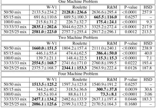
Table 5: Average weighted tardiness for different job mixes. R&M is used as the Force definition for the W-V1 approach. The results are compared to R&M and the simpler randomizing scheme (Roulette). 95% confidence intervals and P-values from ANOVA tests with correlated samples are shown. HSD is the absolute difference between any two means required for significance at the 0.05 level according to the Tukey HSD test.
One Machine Problem
W-V1 Roulette R&M P-value HSD
50/50 mix 2133.5234.2 2128.8236.6 2636.6295.4 <0.0001 257.9
85/15 mix 691.6110.6 689.5100.3 665.5116.0 0.6257 –
100/0 mix 215.831.2 226.732.7 175.424.1 <0.0001 9.3
33/33/33 mix 2835.1202.6 3044.6225.3 3325.2272.4 <0.0001 217.9
50/25/25 mix 2581.0223.0 2757.7255.4 2917.2296.1 0.0012 213.5
Two Machine Problem
W-V1 Roulette R&M P-value HSD
50/50 mix 1660.0151.5 1804.2157.4 2111.0240.1 <0.0001 238.9
85/15 mix 446.155.4 474.462.5 386.450.0 <0.0001 40.0
100/0 mix 139.721.1 148.422.5 115.315.3 <0.0001 7.1
33/33/33 mix 2554.5168.7 2741.6171.0 2760.8199.5 0.0222 193.4
50/25/25 mix 2375.7168.7 2344.1153.3 2563.9222.4 0.0126 187.8
Four Machine Problem
W-V1 Roulette R&M P-value HSD
50/50 mix 1513.5125.2 1597.3123.8 1540.9191.2 0.6257 –
85/15 mix 344.240.2 318.536.6 300.737.8 0.0039 30.6
100/0 mix 83.510.4 88.811.1 73.38.1 <0.0001 3.06
33/33/33 mix 2457.1134.2 2482.6133.9 2637.1197.4 0.0446 183.3
50/25/25 mix 2086.1125.6 2199.3132.2 2170.5164.3 0.1680 –
a point of comparison to determine if the more complicated randomization scheme is doing anything purposeful. First note that for the one machine problem, W-V1 always out-performs Roulette. In the 100/0 job mix case, the difference is statistically significant based on a Tukey HSD test. Also in the 50/25/25 job mix, there is no pairwise significance via the Tukey HSD test between W-V1 and Roulette; however, there is significance between W-V1 and COVERT, but not between Roulette and COVERT. In all other mixes for the one machine problem, no pairwise statistical significance is seen between W-V1 and Roulette. In contrast, other than the 85/15 mix there is always pairwise statistical significance between COVERT and the others.
In the two machine problem W-V1 outperforms Roulette with statistical significance in both the 100/0 mix and 33/33/33 mix. In the other three mixes, no pairwise sta-tistical significance was seen between W-V1 and Roulette. In the four machine problem, W-V1 again outperforms Roulette with statistical significance in the 100/0 mix and the 50/25/25 mix. The pairwise results in the other three job mixes showed no statistical significance between W-V1 and Roulette via Tukey HSD.
Overall, Roulette never does better than W-V1 with sta-tistical significance and even in a couple cases when it does better without statistical significance COVERT outperforms both. W-V1, however, does outperform Roulette in a num-ber of cases with statistical significance and in many of those cases also outperforms COVERT. The equivalent results us-ing R&M show essentially the same thus-ing as can be seen in
Table 5. There is benefit to the “scheduling wasp model” approach to randomization.
Conclusion
In this paper we have shown that randomization of heuris-tics can be beneficial even in dynamic online situations. For the difficult problem of weighted tardiness scheduling with sequence-dependent setups, we have improved upon the performance of state-of-the-art weighted-tardiness dis-patch policies by making decisions stochastically biased by the evaluations of these heuristics rather than using the dis-patch policy directly. Our results show that the “easier” the problem and the less that sequence-dependent setups come into play, the less benefit is obtained through randomization. And furthermore the more that sequence-dependence is an issue and the more difficult the problem then the more ben-efit there is to randomization.
In showing this, we have developed and evaluated a pro-gression of randomization methods for dispatch heuristics on a more/less random scale. These methods have at their foundation a model of self-organized wasp social hierar-chies. Given their differential performance across our exper-imental design, one area of future research interest is to at-tempt to map characteristics of the current state of the prob-lem to a degree of randomness required in the decision. This mapping can then allow us to incorporate a mix of the de-scribed approaches to make some decisions in a more or less stochastic manner. For instance, at some points in our simu-lation all jobs may be of a single type in which case it might
be perhaps better to use the dispatch policy directly; while at other points the mix might be closer to 50/50 (or some equivalent for more than two types) in which case a more random decision but biased by the heuristic might be better. In this manner, we may be able to combine the strengths of the deterministic and stochastic methods.
Another area we wish to explore is the use of our ran-domization scheme as an iterative search strategy, in much the same way as is done in (Bresina 1996; Oddi & Smith 1997) We are also exploring the application of our approach to other scheduling problems in both online and offline en-vironments.
Acknowledgements
This work has been funded in part by the Department of Defense Advanced Research Projects Agency and the U.S. Air Force Rome Research Laboratory under contracts F30602-97-2-0066 and F30602-00-2-0503 and by the CMU Robotics Institute. The views and conclusions contained in this document are those of the authors and should not be in-terpreted as necessarily representing the official policies or endorsements, either expressed or implied, of the Air Force or U.S. Government.
References
Bonabeau, E.; Sobkowski, A.; Theraulaz, G.; and Deneubourg, J. L. 1997. Adaptive task allocation inspired by a model of division of labor in social insects. In Lundh, D., and Olsson, B., eds.,Bio Computation and Emergent Computing. World Scientific. 36–45.
Bresina, J. L. 1996. Heuristic-biased stochastic sampling. InProceedings of the Thirteenth National Conference on Artificial Intelligence and the Eighth Innovative Applica-tions of Artificial Intelligence Conference, Volume One, 271–278. AAAI Press.
Cesta, A.; Oddi, A.; and Smith, S. 2001. A constraint-based method for project scheduling with time windows.
Journal of HeuristicsTo appear.
Cicirello, V. A., and Smith, S. F. 2001. Wasp nests for self-configurable factories. InAgents 2001, Proceedings of the Fifth International Conference on Autonomous Agents. ACM Press.
Lee, Y. H.; Bhaskaran, K.; and Pinedo, M. 1997. A heuris-tic to minimize the total weighted tardiness with sequence-dependent setups.IIE Transactions29:45–52.
Morton, T. E., and Pentico, D. W. 1993.Heuristic Schedul-ing Systems: With Applications to Production Systems and Project Management. John Wiley and Sons.
Oddi, A., and Smith, S. F. 1997. Stochastic procedures for generating feasible schedules. InProceedings of the Fourteenth National Conference on Artificial Intelligence and Ninth Innovative Applications of Artificial Intelligence Conference, 308–314. AAAI Press.
Rachamadugu, R. V., and Morton, T. E. 1982. Myopic heuristics for the single machine weighted tardiness prob-lem. Working Paper 30-82-83, GSIA, Carnegie Mellon University, Pittsburgh, PA.
Raman, N.; Rachamadugu, R. V.; and Talbot, F. B. 1989. Real time scheduling of an automated manufacturing cen-ter. European Journal of Operational Research 40:222– 242.
Theraulaz, G.; Goss, S.; Gervet, J.; and Deneubourg, J. L. 1991. Task differentiation in polistes wasp colonies: A model for self-organizing groups of robots. InFrom An-imals to Animats: Proceedings of the First International Conference on Simulation of Adaptive Behavior, 346–355. MIT Press.
Theraulaz, G.; Bonabeau, E.; and Deneubourg, J. L. 1995. Self-organization of hierarchies in animal societies: The case of the primitively eusocial wasp polistes dominulus christ.Journal of Theoretical Biology174:313–323. Vepsalainen, A., and Morton, T. E. 1987. Priority rules and leadtime estimation for job shop scheduling with weighted tardiness costs.Management Science33:1036–1047. Watson, J. P.; Barbulescu, L.; Howe, A. E.; and Whitley, L. D. 1999. Algorithm performance and problem struc-ture forflow-shop scheduling. InProceedings, Sixteenth National Conference on Artificial Intelligence (AAAI-99), Eleventh Innovative Applications of Artificial Intelligence Conference (IAAI-99), 688–695. AAAI Press.