Combining Stochastic Constraint Optimization
and Probabilistic Programming
From Knowledge Compilation to Constraint Solving
Anna L.D. Latour1, Behrouz Babaki2, Anton Dries2, Angelika Kimmig2, Guy Van den Broeck3, and Siegfried Nijssen4
1
LIACS, Leiden University?
2 Department of Computer Science, KU Leuven 3
Computer Science Department, UCLA
4 ICTEAM, Universit´e catholique de Louvain
[email protected],[email protected]
Abstract. We show that a number of problems in Artificial Intelligence can be seen as Stochastic Constraint Optimization Problems (SCOPs): problems that have both a stochastic and a constraint optimization com-ponent. We argue that these problems can be modeled in a new language, SC-ProbLog, that combines a generic Probabilistic Logic Programming (PLP) language, ProbLog, with stochastic constraint optimization. We propose a toolchain for effectively solving these SC-ProbLog programs, which consists of two stages. In the first stage, decision diagrams are com-piled for the underlying distributions. These diagrams are converted into models that are solved using Mixed Integer Programming or Constraint Programming solvers in the second stage. We show that, to yield linear constraints, decision diagrams need to be compiled in a specific form. We introduce a new method for compiling small Sentential Decision Di-agrams in this form. We evaluate the effectiveness of several variations of this toolchain on test cases in viral marketing and bioinformatics.
1
Introduction
Two important areas in Artificial Intelligence are those ofprobabilistic reasoning
and constraint optimization. Constraint optimization problems involve finding the best assignment to given variables satisfying constraints on these variables. The best-knownprobabilistic inferenceproblems are arguably those that involve calculating the marginal conditional probabilityP(X|Y) for given sets of vari-able assignments X andY in a probability distribution.
In recent years it has become increasingly clear that these areas are closely related to each other. For example: calculating P(X |Y) can be understood as
weighted model counting, i.e., calculating a weighted sum over all assignments to ?The inspiration for this work came during a research visit to the Computer Science
Department of KU Leuven. The work itself was done during a research visit to the ICTEAM institute of Universit´e catholique de Louvain.
variables that satisfy constraints [9]. Similarly, maximum a posteriori (MAP) in-ference, the problem of computing the most likely assignment to given variables in a distribution, can be seen as a constraint optimization task [23]. Optimization problems over distributions are closely linked to constraint optimization prob-lems under soft constraints [4].Mixed networksessentially combine probabilistic graphical models and constraint networks [18].
One combination of constraint programming (CP) and probabilistic inference is the focus of this paper:stochastic constraint programming(SCP) [27], which is closely related tochance constraint programming[8] andprobabilistic constraint programming[25]. The key idea in SCP is to introducestochastic constraintsand
stochastic optimization criteriain CP. An example of a stochastic constraint is that the probability of the occurence of an event should not exceed a threshold. Three key limitations of the state of the art of SCP are the basis for this work. First: most publications on SCP are focused on specific types of prob-lems: scheduling and planning problems, typically (see [1, 17] for some recent examples). Second: there is no generic language for modeling Stochastic Con-straint Optimization Problems (SCOPs). Third: there is no automatic toolchain for solving SCOPs written in such a modeling language. The aim of this work is to advance the state of the art in SCP on these dimensions.
We will use two motivating examples to illustrate that SCP is not only useful in planning and scheduling, but also in data mining and bioinformatics:
Viral marketing [16]. We are given a social network of individuals whose trust relationships are probabilistic: the behaviour of one person inspires each of their friends to do the same with a certain probability. We have budget to distribute marketing material tok nodes in this network. Which people do we target for marketing to such that we (indirectly) influence the largest expected number of people?
Signaling-regulatory pathway inference [21]. We are given a network of genes, proteins and their interactions, where the interactions are probabilis-tic. Furthermore, we are given knock-out pairs: pairs of nodes for which positive or negative change in the expression level of one node is observed when the other node is knocked out. Paths of interactions can explain the positive or negative effect of one node on another. In order to better under-stand these interactions, we want to extract the part of the network that best explains the positive effect (theory compression [13]). We ask: which in-teractions should we select such that in the resulting extracted network the expected number of positive effects is maximized, but the expected number of negative effects is limited by a constant?
Clearly, these problems also involve a combination of constraint optimization and probabilistic reasoning. They can be considered instances of SCP, as they involve finding an assignment to discrete variables, such that a probabilistic optimization criterion is maximized and a probabilistic constraint is satisfied.
A specific property of these problems is however that the decision problem is specified over a very different type of distribution than common in existing SCP systems: probabilistic networks, i.e., networks in which edges exist with a
certain probability. To the best of our knowledge, no tools currently exist for modeling and solving SCOPs in this setting. The second aim of this paper is to introduce a generic system that can be used to model and solve these SCOPs, and potentially many other SCOPs. As common in CP, our proposed system consists of two components: a modeling component and a solving component.
For the modeling component we propose to exploit the fact that in recent years, significant progress has been made in the development ofprobabilistic pro-gramming languages5. These languages allow programmers to program distribu-tions. Until now, however, they have rarely been linked to constraint program-ming. In this paper, we expand a probabilistic programming language, ProbLog [14], which is especially suited for programming distributions over probabilis-tic networks, such that it can be used to formalize SCOPs as well; we call the resulting language SC-ProbLog (Stochastic Constraint Probabilistic Logic Pro-gramming). This extension of ProbLog builds on an earlier version of ProbLog for solving decision-theoretic problems (ProbLog) [26]; compared to DT-ProbLog, SC-ProbLog adds support for hard constraints.
For the solving component we propose to build a toolchain on technology that is taken both from the probabilistic reasoning and constraint programming literature. For the probabilistic reasoning component, we focus on the compila-tion ofSentential Decision Diagrams(SDDs) [12], as they are known to lead to smaller representations of distributions than for instance Ordered Binary Deci-sion Diagrams(OBDDs) [7]. We use these SDDs to generate arithmethic circuits (ACs) and formalize deterministic constraints based on these ACs. For constraint solving we use both CP solvers and Mixed Integer Programming (MIP) solvers. A key technical contribution of this paper is that we show that SDDs need to satisfy strict criteria in order for them to yield linear representations of proba-bilistic constraints. We introduce a new algorithm for minimizing SDDs within this normal form. This allows us to reduce the size of the resulting ACs.
This paper is organized as follows. First, we introduce the range of SCOPs that are the focus of this work, showing by example how problems can be modeled in the proposed SC-ProbLog language. In Sect. 3 we provide background on how probabilities are defined and calculated in ProbLog, which is necessary to understand the first stage of our proposed method. In Sect. 4 we describe our method: we introduce the aforementioned normal form and our new SDD minimization algorithm. Experiments are presented in Sect. 5.
2
Modeling Problems in SC-ProbLog: An Example
As common in (one-stage) SCP [27], we assume given two types of variables:
decision variables(denoted asdi) and mutually independentstochastic variables (denoted asti). The aim is to find an assignment to the decision variables, such that stochastic constraints and optimization criteria are satisfied. Constraints and optimization criteria are considered to be stochastic if their definition in-volves the use of stochastic variables.
5
a b c d pab pbc pbd pcd da db dc dd
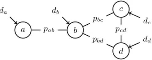
Fig. 1. A social network with a viral marketing problem superimposed on it. Nodes are people, undirected edges indicate trust relationships, where the probability that personi and person jtrust each other is pij. The decision whether or not to target personidirectly is indicated by variabledi.
We consider a limited choice of constraints and variables in this work. First, we restrict our attention to problems in which all variables take Boolean values. As a consequence, each stochastic variable is independently true or false with a given a probability. Second, we only consider constraints of the following kind:
X i rivi ≤θ and/or X i rivi≥θ, (1)
where vi represents either a decision variable di or the conditional probability
Pi(ϕi|σi) that a stochastic Boolean formulaϕi evaluates to true given an as-signment to decision variablesσi. We letri∈IR be a reward for decision variable
di or formulaϕievaluating to true, and letθbe a constant threshold. This con-straint can be thought of as expressing a bound on expected utilities: we sum rewards for events, each of which could happen with a certain probability, given an assignment to the decision variables. Whether an event happens in a cer-tain situation, is expressed using a Boolean logical formulaϕi that includes the stochastic variables; hence the formulaϕiis only true with a certain probability. For reasons of simplicity, we limit ourselves in this paper to the case that
ri= 1, although it is trivial to extend our approach to settings in whichri6= 1. Optimization criteria are of a similar linear form.
The viral marketing problem [16] is an example of a SCOP in this class of SCOPs. We illustrate this on the network of Fig. 1. The nodes represent people; they are either targeted directly in a marketing campaign or not (the decisions). The (undirected) edges represent probabilities that one person trusts another, and vice versa. These probabilities are indicated by variables such aspab on the edges of the graph. We formalize this problem as a SCOP as follows:
– for each nodeiin the graph we create a decision variabledi;
– for each edge (i, j) in the graph we create a stochastic variable tij; the probability that the variabletij is true is equal to that of the edge,pij;
– as constraint we impose the requirement thatP
idi≤k;
– as optimization criterion we use the function P
iP(ϕi|d1, . . . , dn); intu-itively, the aim is that P(ϕi|d1, . . . , dn) represents the conditional prob-ability that node i is reached if an advertisement is sent to exactly those people indicated by the variables d1, . . . , dn. By summing these probabili-ties, we obtain an expected number of persons that is reached.
An important idea is hence to formalize the probability that a person is reached as the probability that some given logical formulaϕi evaluates to true given an assignment to decision variables.
We propose the development of a language, SC-ProbLog, for writing down these constraints and the distributions P(ϕi|d1, . . . , dn) in a systematic man-ner. This language extends the ProbLog language [14, 15]. An example of a pro-gram in SC-ProbLog is given below. Lines 1–9 are written in ProbLog; lines 10–14 are specific to SC-ProbLog. As this example demonstrates, ProbLog’s notation is similar to that of Prolog; its main extension is the ability to add probabilities to facts (lines 5 and 6). These facts become stochastic variables.
1.% Background knowledge 2. person(a). person(c). 3. person(b). person(d). 4.% Probabilistic facts 5. 0.7::directed(a,b). 0.4::directed(b,d). 6. 0.2::directed(b,c). 0.6::directed(c,d). 7.% Relations
8. trusts(X,Y) :- directed(X,Y). buys(X) :- marketed(X). 9. trusts(X,Y) :- directed(Y,X). buys(X) :- trusts(X,Y), buys(Y).
10.% Decision variables 11. ?::marketed(P) :- person(P).
12.% Constraints and optimization criteria 13. { marketed(P) => 1 :- person(P). } 8. 14. #maximize { buys(P) => 1 :- person(P). }.
The example program reflects several assumptions in lines 8–9. First, the trust relationship is bidirectional. Second, if a person is targeted directly, they will certainly buy the product. Third, if a personitrusts another person j and
j buys the product, then ibuys the product.
Traditional ProbLog would allow for the calculation of a success probability for a given query, such as :- buys(a)., based on lines 1–9, for a given set of facts marketed(X).
In the syntax of lines 10–14, we draw inspiration from DT-ProbLog, a version of ProbLog with support for optimization, but not constraints [26], and Answer Set Programming, to formalize constraints. Line 11 defines a decision variable for each person; it defines a search space of facts that can be added to the ProbLog program. Subsequently, we specify optimization criteria and constraints. Line 13 defines a reward (a weightri) of 1 for each person that marketing materials are sent to, and we bound the number of targeted persons to 8. Line 14 adds a prob-abilistic query buys(P). for each person Pto the optimization criterion. Here we effectively maximize the expected number of people that buy the product.
3
Background
To understand the model in the previous setting, and to understand our newly proposed method, it is important to understand in more detail how the calcu-lation of a conditional probability in ProbLog can be formalized as calculating
the probability that a formula over decision variables and stochastic variables evaluates to true. We will use our earlier example to illustrate this. For a full introduction, the reader is referred to the literature [14].
As an example we consider calculating the probability that personain our network buys a product, given decision variables for each person. The key insight is that for the query buys(a), the following grounded formula in Disjunctive Normal Form (DNF) can be constructed:
ϕa=da∨(tab∧db)∨(tab∧tbc∧dc)∨(tab∧tbd∧dd) ∨(tab∧tbd∧tdc∧dc)∨(tab∧tbc∧tcd∧dd),
(2)
This formula can be derived using Selective Linear Definite clause resolution, or SLD-resolution [3, 14], from the original ProbLog program. For example: the clause (tab∧db) reflects the possibility that person a buys the product if it is marketed toband the edge between nodesaandbis present. As earlier,db is a decision variable;tab is a stochastic variable with probabilitypab of being true.
Assume that the product is only marketed to person d. In this case, the formula reduces toϕa= (tab∧tbd)∨(tab∧tbc∧tcd).What is now the probability that person a will buy the product? The key idea that underlies both SCP and ProbLog is that the stochastic variables are considered to be true with a probability that is independent from the other stochastic variables. One possible
model for formula ϕa is: tab =tbd =>, tbc=tcd=⊥. The probability for this model (itsweight) ispab×pbd×(1−pbc)×(1−pcd). Theprobability of the query
ϕa is defined to be sum of the weights of all the models of the above formula. Hence, this problem is aweighted model counting(WMC) problem [9].
Calculating the WMC by enumerating all models is usually not efficient. A more efficient calculation is the following:pab×pbd+pab×(1−pbd)×pbc×pcd. The first product corresponds to the first possible path, the second product to the second path. Note that this formula includes a term (1−pbd). This term is necessary as we would otherwise count the model tab =tbd =tbc =tcd=> twice. This problem is known as the disjoint sumproblem.
As the previous example makes clear, computing the probability of a DNF formula is hard due to the disjoint sum problem; in general, it is known to be #P-complete [24]. This makes solving this type of SCP particularly hard. How-ever, several practical approaches have been proposed to make WMC feasible in practice. One such approach is based oncompilingthe logical formula into a deci-sion diagram, and constructing an AC from this diagram [11]. Two well-studied types of decision diagrams areOrdered Binary Decision Diagrams(OBDDs) [7] andSentential Decision Diagrams (SDDs) [12]. The latter type of decision dia-grams has recently been shown to generalize OBDDs, and can be exponentially more compact [6]. For this reason, we focus on SDDs.
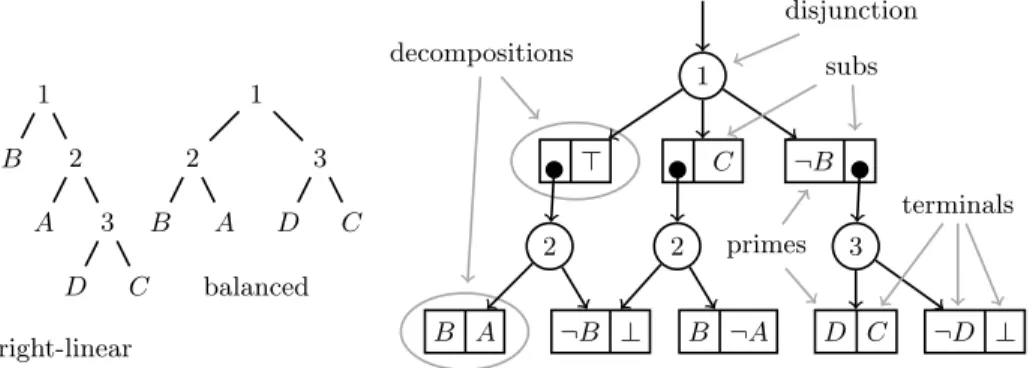
An SDD consists of decompositions, disjunctions and terminals (see Fig. 2 for an example SDD for a formulaf that is similar to the formula considered earlier, but that illustrates the concept of SDDs better). A decomposition consists of a
primepand asubs, and one decomposition represents the logical formula (p∧s). Disjunction nodes represent the disjunction of two or more decompositions. The
1 B 2 A 3 D C right-linear 1 B 2 A 3 D C balanced 1 > C ¬B 2 2 3 B A ¬B ⊥ B ¬A D C ¬D ⊥ disjunction primes subs terminals decompositions
Fig. 2.Two examples of vtrees (left, center), each for variable orderB < A < D < C. An SDD (right) for logic formulaf= (A∧B)∨(B∧C)∨(C∧D), which respects the balanced vtree. Example from Darwiche [12].
shape of the SDD is completely determined by a tree structure over the variables present in it. This tree structure is called avtree [22]. Two examples of vtrees are given in Fig. 2. A vtree induces atotal variable orderfor an SDD when traversed from left to right. We now discuss how vtrees relate to SDDs.
All disjunctions are required torespect specific nodes in the corresponding vtree. A disjunction respects a vtree nodeiif for all its child decompositions, each variable occurring in the sub-SDD rooted at the prime (sub) of the decomposition occurs in the sub-vtree rooted at the left (right) child ofi. Thus, the disjunctions labeled ‘2’ in Fig. 2 each respect vtree node 2 in the balanced vtree shown in the same figure. An SDD that respects a right-linear vtree is essentially an OBDD [12]; hence, SDDs generalize OBDDs. As with OBDDs, the size of an SDD is influenced by the total variable order that is induced by the vtree it respects. The shape of the vtree also influences the size of that SDD.
Once the SDD is compiled, WMC can be performed in time linear in the size of the SDD. In a bottom-up fashion the SDD is first turned into anarithmetic circuit (AC). In this AC, we assign the appropriate probabilities and decision values to the leafs of the circuit. The transformation of the SDD into an AC is simple: each decomposition node is replaced by a product node between its prime and its sub; each disjunction node is replaced by a summation node over the child nodes.6The properties of an SDD ensure that the disjoint sum problem is taken care of in the resulting circuit.
4
Approach
We first make some observations, then aggregate them in a proposed algorithm. 6 This method was used for counting models of a Boolean formula in decomposable
Deterministic Negation Normal Form (d-DNNF)[11], and can be applied to SDDs because SDDs are a proper subset of d-DNNFs [12].
SCOP solving with MIP solvers. Given an SC-ProbLog program that models a certain SCOP instance, the naive way of solving this SCOP is the following. Compile each of the queries present in the program into an AC containing de-cision variables and stochastic variables. For each possible assignment to the decision variables, fill in their values in the AC. Calculate the probabilities using the AC. Use the resulting probabilities to compute the objective value and to check for constraint satisfaction. Continue until the optimal strategy is found.
Given that the number of possible assignments is exponential in the num-ber of decision variables, this approach is feasible for none but the smallest of problems. A more efficient approach may be to encode the AC in a constraint programming model, similar to [2], and to use a CP solver on the resulting model. We explore a new approach, which involves mapping the SDD into a mixed integer programming (MIP) model.
From SDD to MIP model. Mapping arithmethic circuits into quadratic programs is relatively easy. Essentially, we introduce an additional variable for each node in the AC, which we constrain to equal the product or the sum of its children.
For MIP solvers the quadratic constraints in this na¨ıve model can however be problematic. As the constraints can be shown to be nonpositive semidefinite, we cannot apply QCQP solvers either. It is important that we are able tolinearize
the products in our model, i.e., that we can transform the model in a set of equivalent linear constraints. As a short reminder, a constraint of the forma=
b×c can be linearized in these cases7: (1) at least one of the two variables in {b, c} is a constant; (2) at least one of the two variables in {b, c} is a Boolean variable. Therefore, we need to ensure that in a decomposition node of the SDD, variables representing the two children satisfy these requirements.
Special vtrees. Next, we show that it suffices to constrain the vtrees to ensure that SDDs can be linearized. Recall that for each SDD decomposition node, the respected vtree determines the variables that can occur in the prime and in the sub. We observe the following: if all left-hand (right-hand) descendants of an internal vtree nodenare stochastic variables, then for each SDD decomposition nodemwhose parent respectsn, it holds that all variables occuring inm’s prime (sub) are stochastic as well. A similar property holds for decision variables.
If a prime contains only probabilities, which can be considered as constants for the model, we can precompute the corresponding value for the prime, effec-tively eliminating the MIP model variable associated with that prime. Similarly: since we can linearize all operations on Boolean variables [19], any prime con-taining only decision variables can be expressed by a Boolean variable with linear relations to other variables. Thus, in each of these two cases, the expression rep-resented by the prime can be linearized and hence the product reprep-resented by the SDD decomposition node as well. The same holds for subs.
This leads us to define the concept ofmixed and pure nodes in a vtree. A
purenode is an internal node whose leaf descendants all are variables of the same 7
type (either stochastic or decision), while amixed node is an internal node that has leaf descendants of both types. We state that an SDD can be linearized into a MIP model if the vtree that it respects has thesingle mixed path property.
Definition 1. Given a vtree on variables of two distinct classes (e.g. decision and stochastic). This vtree has the single mixed path (SMP) property (and is called an SMP vtree) if, for each of its internal nodes n, the following holds: either both children of nare pure nodes, or one child ofnis pure and the other child is mixed. As a consequence, if an SMP vtree has mixed nodes, all mixed nodes occur on the same path from the root of the vtree to the lowest mixed node. Minimizing SDDs. Recall that SDDs that respect right-linear vtrees are es-sentially OBDDs. One can easily verify that a right-linear vtree has the SMP property: if it has an SMP, it is on the right spine of the vtree. From this fol-lows that OBDDs can be linearized. However: right-linear vtrees generally do not yield the smallest SDDs. Since the size of the SDD determines the size of the resulting MIP model, and thus the solving time, small SDDs are preferable as input for the MIP model builder.
Choi and Darwiche have proposed a local search algorithm for SDD minimiza-tion [10]. This algorithm considers three operaminimiza-tions on the vtree: right-rotate,
left-rotate (each well-known operations on binary trees) andswap. When a swap operation is applied to an internal node, the sub vtrees rooted at its children are swapped. Given a (sub) vtree, the greedy local search algorithm of Choi and Darwiche loops through its neighbourhood of different vtrees by applying con-secutive rotate and swap operations, trying to find a vtree that yields a smaller SDD. Since OBDD minimization is NP-hard [5], we expect SDD minimization to also be NP-hard, but we are not aware of any published proof of this.
Generally, this minimization produces vtrees that donothave the SMP prop-erty, even if the initial vtree did; the rotate moves may remove this property.
A desirable property of Choi and Darwiche’s algorithm is the following: the three local moves considered are sufficient to turn anyvtree on a certain set of variables into any other vtree on the same set of variables. Consequently, the local moves in principle allow complete traversal of the search space of vtrees.
Here, we propose a simple modification of Choi and Darwiche’s algorithm: we use the same local moves as their algorithm does, but any move that leads to a vtree that violates the SMP property is immediately rejected.
While this modification is conceptually easy, a relevant fundamental question is whether under this modification it is still possible to traverse the space of SMP vtrees on a fixed set of variables completely. We show that this is indeed the case. In the following we refer to the leaf node that represents the variable that is lowest in the order associated with a vtree asLL(lowest leaf).
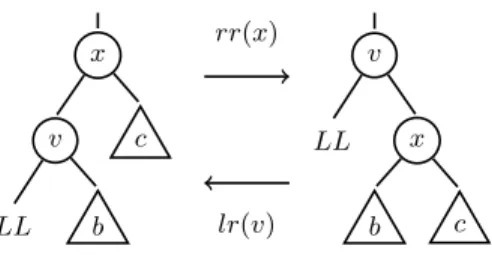
Lemma 1. Let v be the parent and x the grandparent of the LL in an SMP vtree. Right rotate on xmaintains the SMP property for the vtree rooted atv. Proof. Consider the left SMP vtree in Fig. 3. Given that this vtree satisfies the SMP property by assumption, sub vtreesbandccannot both be mixed, but one of them can be. Now consider the following cases:
x v LL b c rr(x) lr(v) v LL x b c
Fig. 3. Rotate operations on an SMP vtree. Node LL is the lowest variable in the variable induced by these vtrees. Nodesvandxare internal;bandcare sub vtrees.
Both b and c are pure and of the same class as LL: Lemma 1 holds triv-ially.
Both b and c are pure, not each of the same class as LL: Any class as-signment tob andcwill preserve the SMP property.
Node b is pure, node c is mixed: Sincebis of the same class as LL(by as-sumption), nodev is pure and nodexis mixed. After applying right-rotate on nodev, both vandxare mixed, and the SMP property is preserved.
Node b is mixed, node c is pure: Nodeccan belong to any class, since both nodev and nodexare mixed before as well as after applying right-rotate to
v, preserving the SMP property under rotation.
Note that the SMP vtree described above may be a sub vtree of a larger vtree. The fact that the right-rotate operation does not change the nature (mix or pure) of the root of this sub vtree, leads to the following corollary:
Corollary 1. A right-rotate operation on the grandparent of the LL node does not change the SMP status of the full vtree.
Lemma 2. Given an SMP vtree with nodeLL in orderO. We can always ob-tain an SMP vtree on the same order O in which the LL is the left child of the root, through a series of right-rotate operations, without ever in the process transforming it into a vtree that violates the SMP property.
Proof. A right-rotate operation on an internal vtree node decreases its left child’s distance to the root of the vtree by one. Repeated applications of right-rotate on
LL’s grandparent ultimately makes LL’s parent the vtree’s root. By Lemma 1 and Corrolary 1, the SMP status of the vtree never changes in this process.
Lemma 3. Given an SMP vtree on orderO, we can always obtain a right-linear vtree on the same order, through a series of right-rotate operations, without ever in the process transforming it into a vtree that violates the SMP property. Proof. By Lemma 2 we can turn any SMP vtree in one for which theLLis the left child of the root. This vtree can be made right-linear by recursively applying this method to the root’s right child.
Lemma 4. A right-linear SMP vtree with variable orderO can be transformed in any SMP vtree on the same variable order by a series of left-rotate operations without ever in the process transforming into a vtree without the SMP property. Proof. Since left-rotate is the dual operation of rotate, a sequence of right-rotate moves transforming any vtree to a right-linear one through right-right-rotate operations, can simply be reversed through left-rotate operations to turn a right-linear vtree in any other (on the same variable order).
Note that rotate operations preserve the variable order in the vtree, only chang-ing its shape. However, the space of possible vtrees on a fixed set of variables is larger, since different variable orders exist. The order of variables is changed by the application of swap operations.
Lemma 5. Any right-linear vtree on variable order O can be transformed into a right-linear vtree on any other variable order O0 through a series of rotate and swap operations without ever in the process transforming into a vtree that violates the SMP property.
Proof. Observe that any right-linear vtree satisfies the SMP property. Observe that if we can reverse the mutual order of two adjacent variables (e.g. A < B < C < D becomes A < C < B < D), we can create any variable order by repeatedly reversing the orders of adjacent variables.
This order reversal is simple. Suppose that nodebin the right vtree of Fig. 3 is a single variable, as isLL. We can makeLL andbswap places by applying a left-rotate onv, resulting in the left vtree of Fig. 3, and then applying a swap operation onv, followed by a right-rotate operation onx.
Theorem 1. Any SMP vtree can be transformed into any other SMP vtree on the same variable through a series of rotation and swap moves, without ever in the process transforming into a vtree that does not have the SMP property.
We conclude that an SMP-preserving minimization algorithm that applies only swap and rotate operations can in principle convert any SMP vtree into any other SMP vtree on the same variables.
Summary. These observations spark the following algorithm for solving SCOPs: 1. ground formulas for the queries present in the SCOP;
2. compile SMP vtree respecting SDDs for all these queries (ProbLog’s default mechanism uses right-linear vtrees, so this is automatically satisfied); 3. apply the SMP-preserving local search algorithm to minimize these SDDs; 4. convert the SDDs into arithmetic circuits and then into sets of constraints; 5. add the optimization criterion and linear constraints of the SCOP to the MIP model, ensuring e.g. that for an upper-bounded stochastic constraint the model variables representing the root of each relevant query are added using a linear model constraint of the formP
irivi≤θ; 6. apply a MIP solver or a CP solver to find a solution.
For CP solvers, the unconstrained minimization algorithm can be used to obtain smaller SDDs. ProbLog’s compilation strategy yields SDDs respecting right-linear vtrees. Thus, without minimization, the SDDs are essentially OBDDs.
5
Experiments
We state some questions that we wish to answer for the approach described in the previous section. Then we describe the experiments we use to answer these questions.
Questions. Recall that the size of a MIP or CP model is linear in the size of the SDDs it is built on. We expect smaller models to be faster to solve. However: minimizing an SDD takes time. Furthermore, when quadratic constraints are allowed, we expect to obtain smaller SDDs; however, solving quadratic problems using CP may take longer than solving MIPs. We pose the following questions:
(Q2) How do SDD sizes depend on the choice of minimization algorithm?
(Q3) How do the calculation times for the full toolchain compare for CP and MIP solvers, with and without appropriate minimization?
(Q4) How do the computation times for different phases of the algorithm com-pare to each other?
To answer these questions, and to demontrate that SC-ProbLog programs can be solved in practice, we apply our algorithms to different SCOPs. Of course, the constraints determine problem hardness, which begs the question:
(Q1) Which threshold settings are useful for an evaluation of the solving times?
Description of Test Data. Our experiments focus on two types of real data sets: a social network and a gene-protein interaction network. As social network
we use the High-energy theory collaborations network [20], which was also used in earlier publications on viral marketing [16]. This collaboration network of 7610 authors (nodes) has 15751 undirected weighted edges, which we turn into probabilities following Kempe’s approach [16]. Initial experiments showed that the full network is too large to ground the problem’s programs. We useGephi’s8 implementation of the Louvain algorithm for weighted community detection to extract communities. We consider two specific communities, referred to as hep-th47andhep-th5. Compared to our earlier viral marketing ProbLog program, in our experiments we include additional stochastic variables such that a person does not automatically buy a product if it is marketed to them.
AsDNA-protein and protein-protein interaction networkwe use the
Signaling-regulatory Pathway INference [21] (or SPINE) network, with 4696 nodes representing genes and proteins. It contains 15147 undirected protein-protein edges, and 5568 directed protein-protein-gene edges. The set provides probabili-ties for both the undirected protein-protein edges, and the directed protein-gene edges. We again useGephi’s community detection, where we take care to ensure that both negative and positive knockout pairs are contained in our samples. We consider models referred to asspine16andspine27in our experiments. We use a specific path definition that requires paths to end in a protein-DNA edge.
8
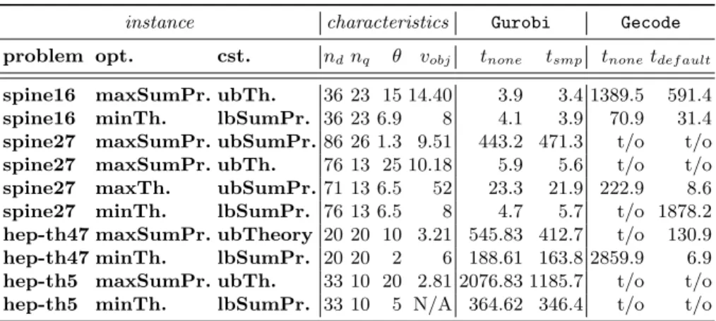
Table 1. Performance in seconds of the different methods on the hardest instances of the testcases for the full toolchain. We give the problem set, optimization and con-straint setting, number of decision variables nd, number of ProbLog queriesnq that comprise the objective function and/or constraint, thresholdθand objective valuevobj
(N/A denotes a problem that has no solution for that threshold). We show the solving times for the default SDD with no minimization (tnone), SMP minimization (tsmp) and default minimization (tdef ault) forGurobiandGecode. We indicate a timeout with t/o.
instance characteristics Gurobi Gecode
problem opt. cst. ndnq θ vobj tnone tsmp tnonetdef ault
spine16 maxSumPr. ubTh. 36 23 15 14.40 3.9 3.4 1389.5 591.4
spine16 minTh. lbSumPr. 36 23 6.9 8 4.1 3.9 70.9 31.4
spine27 maxSumPr. ubSumPr.86 26 1.3 9.51 443.2 471.3 t/o t/o
spine27 maxSumPr. ubTh. 76 13 25 10.18 5.9 5.6 t/o t/o
spine27 maxTh. ubSumPr. 71 13 6.5 52 23.3 21.9 222.9 8.6
spine27 minTh. lbSumPr. 76 13 6.5 8 4.7 5.7 t/o 1878.2
hep-th47 maxSumPr. ubTheory 20 20 10 3.21 545.83 412.7 t/o 130.9
hep-th47 minTh. lbSumPr. 20 20 2 6 188.61 163.8 2859.9 6.9
hep-th5 maxSumPr. ubTh. 33 10 20 2.81 2076.83 1185.7 t/o t/o
hep-th5 minTh. lbSumPr. 33 10 5 N/A 364.62 346.4 t/o t/o
Optimization and Constraint Settings. We consider several combinations of op-timization and constraint settings on the programs described above. We use the following abbreviations.maxSumProbdenotes a maximization over stochastic variables, whilemaxTheory denotes a maximization over the sum of decision variables set to true (theory size). For constraints we use these abbreviations:
ubSumProbdenotes a constraint in which we impose an upper bound on an ex-pectation;ubTheorydenotes a constraint in which we impose an upper bound on the theory size. We also define minimization and lower bound counterparts of these settings. Table 1 lists the four datasets that we use, along with the tasks we evaluate on each dataset. For instance, the combination (maxSumProb,
ubTheory) is the viral marketing setting we considered earlier in this paper.
Software And Hardware. We use Gurobi 6.52 as MIP solver andGecode 5.0.0 as CP solver9. For each phase of the toolchain (grounding of the program, SDD compilation, building of the constraint model and solving it) we use a timeout on our experiments of 3600s. They were implemented inPython 3.4, usingProbLog 2.110for the grounding of programs.ProbLog 2.1uses version 1.1.1 of UCLA’s sddlibrary11, which is implemented in C, for SDD compilation. They were run on a machine with an Intel Xeon E5-2630 processor and 512GB RAM, under Red Hat 4.8.3-9.
9 Available atwww.gurobi.comandwww.gecode.org. 10
Availabe athttps://dtai.cs.kuleuven.be/problog/.
11
0 5 10 15 20 threshold [theory size] 0 500 tim e [s ]
Fig. 4. Example of performance of
Gurobi with non-minimized SDD on dif-ferent thresholds, for problem hep-th47
withmaxSumProb,ubTheory.
0 25 50 75 without minimization [x 10,000] 0 20 40 60 80 w it h m in im iz a tio n [x 1 0 ,0 0 0 ] equal size smp default
Fig. 5. Comparison of size reduction by SDD minimization algorithms. 0 20 40 60 without minimization [s] 0 20 40 60 w it h m in im iz a tio n [s ] equal time smp default
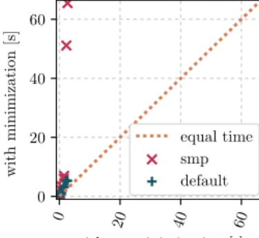
Fig. 6. Comparison of SDD compilation times. 0 1000 2000 without minimization [s] 0 1000 2000 w it h m in im iz a tio n [s
] equal timesmp (Gurobi)
default (Gecode)
Fig. 7.Comparison of full toolchain solv-ing times for the two solvers.
Results. To answer(Q1), Fig. 4 shows solving times for thehep-th47problem in the (maxSumProb,ubTheory) setting, for different thresholds. As expected, we find that thresholds that are not very strict or loose, require the longest solving times. We performed similar experiments for the other problem settings to systematically identify the threshold for which each problem was the hardest, which we then chose as test cases for the SCOP solving method comparison.
To answer(Q2), Fig. 5 shows a comparison of the size reductions obtained by the SMP-minimization algorithm and the default minimization algorithm provided by the sdd library. We find that the SMP minimization algorithm typically halves the size of the initial SDD. The default minimization typically reduces the size of the SDD by one or two orders of magnitude.
To answer(Q3), we summarize the performance of the four methods on our test cases in Table 1. For the hep-th5 problem we selected the ten highest-degree nodes for the queries, since the program could not be grounded within one hour if we selected all 33 nodes in the problem for querying. This reduced the
grounding time to about 112 seconds. For the other test cases we have selected all queries in the problem, with grounding times in the range of 1–5 seconds.
We observe that without any minimization of the SDD,Gurobiconsistently outperformsGecode. Furthermore, we observe that the difference made by SDD minimization is larger for the Gecode methods than for the Gurobi methods. This can largely be explained by the results in Fig. 5, and by those in Fig. 6, which answer question(Q4). The latter show that generally, compiling SDDs is a matter of seconds, whether they are being minimized or not. The exception is thehep-th5problem, which takes tens of seconds to compile into an SDD when using SMP minimization. Observe from the table that minimization is still useful here, as it reduces solving time enough to make up for the extra minimization time. We note that the minimization algorithms are based on heuristics, and minimization speed-up may lie in the improvement of these heuristics.
Finally, Fig. 7 shows that the time that is gained during the optimization part of the entire solving chain, can be orders of magnitude larger than the time lost by minimizing the SDD. We do note that, since compiling the SDD can be done in seconds, this effect is less noticable for the smaller problems.
6
Conclusions
We introduced a specific class of SCOPs, in which we can impose constraints and optimization criteria based on expected utilities over probabilistic programs. We demonstrated that a viral marketing problem and a problem in bioinformatics can be considered instances of such SCOPs. We showed how generic probabilistic programming technology can be combined with constraint optimization solvers to solve these problems, and introduced an SDD minimization algorithm that preserves properties that ensure linearizability of the SDD to a MIP model, while reducing the size of the SDD. While the results are encouraging, an important remaining challenge is scalability; local search and sampling algorithms could be of interest here for the probability calculation, the optimization, and the minimization of circuit sizes. We believe that the methods here presented can also be applied in other contexts than those studied here. Many possibilities remain for the further integration of CP and probabilisic programming, given the limitations on the type of constraints and probabilistic models considered in this work.
Acknowledgements. We thank Luc De Raedt for his support, for his advice and for the numerous other ways in which he contributed to this work. This research was supported by the Netherlands Organisation for Scientific Research (NWO) and NSF grant #IIS-1657613.
References
1. Babaki, B., Guns, T., De Raedt, L.: Stochastic constraint programming with and-or branch-and-bound
2. Babaki, B., Guns, T., Nijssen, S., De Raedt, L.: Constraint-Based Querying for Bayesian Network Exploration. In: Advances in Intelligent Data Analysis XIV - 14th International Symposium, IDA 2015, Saint Etienne, France, Octo-ber 22-24, 2015, Proceedings. pp. 13–24 (2015), http://dx.doi.org/10.1007/ 978-3-319-24465-5_2
3. Ben-Ari, M.: Mathematical Logic for Computer Science. Springer Publishing Com-pany, Incorporated, 3rd edn. (2012)
4. Bistarelli, S., Rossi, F.: Semiring-Based Soft Constraints. In: Concurrency, Graphs and Models, Essays Dedicated to Ugo Montanari on the Occasion of His 65th Birthday. pp. 155–173 (2008),http://dx.doi.org/10.1007/978-3-540-68679-8_ 11
5. Bollig, B., Wegener, I.: Improving the variable ordering of obdds is np-complete. IEEE Trans. Comput. 45(9), 993–1002 (Sep 1996)
6. Bova, S.: Sdds are exponentially more succinct than obdds. In: Proceedings of the Thirtieth AAAI Conference on Artificial Intelligence. pp. 929–935. AAAI’16, AAAI Press (2016)
7. Bryant, R.E.: Graph-Based Algorithms for Boolean Function Manipulation. IEEE Trans. Computers 35(8), 677–691 (1986)
8. Charnes, A., Cooper, W.W.: Chance-constrainted programming. Management Sci-ence 6, 73–79
9. Chavira, M., Darwiche, A.: On Probabilistic Inference by Weighted Model Count-ing. Artif. Intell. 172(6-7), 772–799 (Apr 2008)
10. Choi, A., Darwiche, A.: Dynamic Minimization of Sentential Decision Diagrams. In: Proceedings of the Twenty-Seventh AAAI Conference on Artificial Intelligence. pp. 187–194. AAAI’13, AAAI Press (2013)
11. Darwiche, A.: On the tractable counting of theory models and its application to truth maintenance and belief revision. Journal of Applied Non-Classical Logics 11(1-2), 11–34 (2001)
12. Darwiche, A.: SDD: A New Canonical Representation of Propositional Knowledge Bases. In: Proceedings of the Twenty-Second International Joint Conference on Artificial Intelligence - Volume Volume Two. pp. 819–826. IJCAI’11, AAAI Press (2011)
13. De Raedt, L., Kersting, K., Kimmig, A., Revoredo, K., Toivonen, H.: Compressing probabilistic Prolog programs. Machine Learning 70(2), 151–168 (2008)
14. De Raedt, L., Kimmig, A., Toivonen, H.: ProbLog: A Probabilistic Prolog and Its Application in Link Discovery. In: Proceedings of the 20th International Joint Conference on Artifical Intelligence. pp. 2468–2473. IJCAI’07, Morgan Kaufmann Publishers Inc., San Francisco, CA, USA (2007)
15. Fierens, D., Van den Broeck, G., Renkens, J., Shterionov, D., Gutmann, B., Thon, I., Janssens, G., De Raedt, L.: Inference and learning in probabilistic logic pro-grams using weighted boolean formulas. Theory and Practice of Logic Program-ming 15(03), 358–401 (2015)
16. Kempe, D., Kleinberg, J., Tardos, ´E.: Maximizing the Spread of Influence Through a Social Network. In: Proceedings of the Ninth ACM SIGKDD International Con-ference on Knowledge Discovery and Data Mining. pp. 137–146. KDD ’03, ACM, New York, NY, USA (2003)
17. Lombardi, M., Milano, M.: Allocation and scheduling of conditional task graphs. Artif. Intell. 174(7-8), 500–529 (2010), https://doi.org/10.1016/j.artint. 2010.02.004
18. Mateescu, R., Dechter, R.: Mixed deterministic and probabilistic networks. Ann. Math. Artif. Intell. 54(1-3), 3–51 (2008), http://dx.doi.org/10.1007/ s10472-009-9132-y
19. McKinnon, K.I.M., Williams, H.P.: Constructing integer programming models by the predicate calculus. Annals of Operations Research 21(1), 227–245 (1989) 20. Newman, M.E.J.: The structure of scientific collaboration networks. Proceedings
of the National Academy of Sciences 98(2), 404–409 (2001)
21. Ourfali, O., Shlomi, T., Ideker, T., Ruppin, E., Sharan, R.: SPINE: a framework for signaling-regulatory pathway inference from cause-effect experiments. Bioinfor-matics 23(13), i359–i366 (2007)
22. Pipatsrisawat, K., Darwiche, A.: New compilation languages based on structured decomposability. In: Proceedings of the 23rd National Conference on Artificial Intelligence - Volume 1. pp. 517–522. AAAI’08, AAAI Press (2008)
23. Riedel, S.: Improving the Accuracy and Efficiency of MAP Inference for Markov Logic. In: UAI 2008, Proceedings of the 24th Conference in Uncertainty in Artificial Intelligence, Helsinki, Finland, July 9-12, 2008. pp. 468–475 (2008),http://dblp. uni-trier.de/rec/bib/conf/uai/Riedel08
24. Roth, D.: On the Hardness of Approximate Reasoning. Artif. Intell. 82(1-2), 273– 302 (Apr 1996)
25. Tarim, S.A., Hnich, B., Prestwich, S.D., Rossi, R.: Finding reliable solutions: event-driven probabilistic constraint programming. Annals OR 171(1), 77–99 (2009),
http://dx.doi.org/10.1007/s10479-008-0382-6
26. Van den Broeck, G., Thon, I., van Otterlo, M., De Raedt, L.: DTPROBLOG: A Decision-theoretic Probabilistic Prolog. In: Proceedings of the Twenty-Fourth AAAI Conference on Artificial Intelligence. pp. 1217–1222. AAAI’10, AAAI Press (2010)
27. Walsh, T.: Stochastic Constraint Programming. In: Proceedings of the 15th Eure-opean Conference on Artificial Intelligence, ECAI’2002, Lyon, France, July 2002. pp. 111–115 (2002)