ARROW@TU Dublin
ARROW@TU Dublin
Dissertations School of Computing
2019
Forecasting Anomalous Events And Performance Correlation
Forecasting Anomalous Events And Performance Correlation
Analysis In Event Data
Analysis In Event Data
Sonya Leech [Thesis]Technological University Dublin
Follow this and additional works at: https://arrow.tudublin.ie/scschcomdis
Part of the Computer Engineering Commons, and the Computer Sciences Commons
Recommended Citation Recommended Citation
Leech, S. (2019) Forecasting Anomalous Events And Performance Correlation Analysis In Event Data, Masters Thesis, Technological University Dublin.
This Theses, Masters is brought to you for free and open access by the School of Computing at ARROW@TU Dublin. It has been accepted for inclusion in Dissertations by an authorized administrator of ARROW@TU Dublin. For more information, please contact
[email protected], [email protected], [email protected].
This work is licensed under a Creative Commons Attribution-Noncommercial-Share Alike 3.0 License
Performance Correlation Analysis In
Event Data
Sonya Leech
A dissertation submitted in partial fulfilment of the requirements of
Dublin Institute of Technology for the degree of
M.Sc. in Computing (Data Analytics)
Date: 01-06-2019
from the work of others save and to the extent that such work has been cited and acknowledged within the text of my work.
This dissertation was prepared according to the regulations for postgraduate study of the Dublin Institute of Technology and has not been submitted in whole or part for an award in any other Institute or University.
The work reported on in this dissertation conforms to the principles and requirements of the Institute’s guidelines for ethics in research.
Classical and Deep Learning methods are quite common approaches for anomaly de-tection. Extensive research has been conducted on single point anomalies. Collective anomalies that occur over a set of two or more durations are less likely to happen by chance than that of a single point anomaly. Being able to observe and predict these anomalous events may reduce the risk of a server’s performance. This paper presents a comparative analysis into time-series forecasting of collective anomalous events using two procedures. One is a classical SARIMA model and the other is a deep learning Long-Short Term Memory (LSTM) model. It then looks to identify if an influx of message events have an impact on CPU and memory performance.
The findings of the study conclude that SARIMA was suitable for time series modeling due to the elimination of heteroskedasticity once transformations were implemented, however it was not suitable for anomaly detection based on an existing level shift in the data. The deep learning LSTM model resulted in more accurate time-series predictions with a better ability to be able to handle this level shift. The findings also concluded that an influx of event messages did not have an impact on CPU and memory performance.
Signed: Sonya Leech
Keywords: ARIMA, SARIMA, LSTM, Anomaly, Collective, Forecasting, Time Series Modelling
I would like to express my sincere thanks to my college supervisor Dr. Bojan Bozic for his guidance, support and tremendous encouragement throughout this work. I would also like to thank Dr. Jonathan Dunne who is our companies data science architect for his outstanding guidance and support throughout this project. He has been an encyclopedia of knowledge. His continued guidance and support has helped me realize that anything is possible once you have patience, dedication and little time on your hands. Without his efforts, I would not have achieved so much. I would also like to wholeheartedly thank my partner Glenn for the endless nights he has been left on his own while I plugged away at getting through college. Not forgetting my father he has been my rock, always there to take the reigns when life gets in the way and his encouragement has helped me keep going and not give up.
Declaration I
Abstract II
Acknowledgements II
0.1 Acknowledgements . . . III
Contents IV
List of Figures VIII
List of Tables X
List of Acronyms XIII
1 Introduction 2
1.1 Problem Statement . . . 3
1.2 Organisation of Dissertation . . . 4
1.3 Scope and Limitations . . . 5
1.3.1 Scope . . . 5
1.3.2 Limitations . . . 5
2 Literature Review 7 2.1 Classification . . . 7
2.2 Time Series Models . . . 8
2.6 Anomaly Detection . . . 18
2.7 Model Evaluation . . . 19
2.8 Summary of Literature . . . 20
2.9 Gaps in Literature . . . 21
2.10 Research Aim and Objective . . . 21
2.10.1 Research Question . . . 21 2.10.2 Research Aim . . . 22 2.10.3 Objective . . . 22 2.10.4 Research Methodologies . . . 23 3 Data Understanding 25 3.1 Feature Identification . . . 26 3.2 Data Cleansing . . . 27 3.3 Missing Data . . . 27 4 Exploratory Analysis 28 4.1 Daily Analysis . . . 29 4.1.1 Normality . . . 30
4.1.2 Unit Root Tests . . . 32
4.1.3 Seasonality & Trends . . . 35
4.1.4 Correlation . . . 37
4.2 Hourly Analysis . . . 38
4.2.1 Normality . . . 38
4.2.2 Stationarity . . . 40
4.2.3 Seasonality & Trend . . . 41
4.2.4 Correlation . . . 42
4.2.5 Cross Correlation . . . 43
5.2.1 Info Hourly ARIMA Analysis . . . 48
5.2.2 Warn Hourly ARIMA Analysis . . . 52
5.2.3 Error Hourly ARIMA Analysis . . . 54
5.2.4 Info Hourly Prediction Analysis . . . 55
5.3 LSTM . . . 58
5.3.1 Info Hourly LSTM Analysis . . . 58
5.3.2 Info LSTM Prediction Analysis . . . 59
6 Anomaly Detection 62 6.0.1 ARIMA . . . 63
6.0.2 LSTM . . . 65
7 CPU-Memory - Performance Analysis 67 7.1 CPU . . . 67 7.2 Memory . . . 69 8 Evaluation 71 8.1 Daily . . . 71 8.1.1 Info . . . 72 8.1.2 Warn . . . 73 8.1.3 Error . . . 74 8.2 Hourly . . . 75 8.2.1 Info . . . 75 8.2.2 Warn . . . 76 8.2.3 Error . . . 77
8.3 Daily - Hourly Recap . . . 78
8.4 Time Series Modelling . . . 80
8.4.1 Info . . . 80
8.5.1 SARIMA . . . 82 8.5.2 LSTM . . . 83 8.5.3 Comparison . . . 84
9 Conclusion and Future Work 85
3.1 Anomaly Detection Architectural Diagram . . . 26
4.1 Exploratory Analysis Dashboard . . . 29
4.2 Info, Warn, Error Daily Distribution Analysis . . . 30
4.3 Daily Quantile Plots . . . 30
4.4 Daily Seasonal Decomposition Analysis . . . 35
4.5 Daily ACF PACF . . . 36
4.6 Daily Pearson Correlation Test : Info : Warn : Error . . . 37
4.7 Hourly Distribution Analysis . . . 38
4.8 Hourly Seasonality-Trend . . . 41
4.9 Hourly ACF-PACF . . . 42
4.10 Hourly Cross Correlation . . . 43
5.1 Un-Transformed Hourly LjungBox Test . . . 48
5.2 Info Hourly ARIMA Analysis log(x) . . . 51
5.3 Warn Hourly ARIMA Analysis log(x) . . . 53
5.4 Error Hourly ARIMA Analysis Square Root . . . 55
5.5 Info Hourly Train And Prediction Result . . . 56
5.6 Info ARIMA Predictions Before Shift In Data . . . 57
5.7 Info ARIMA Predictions After Shift In Data . . . 57
5.8 Info LSTM Model Univariate Walk Forward Box Plot Analysis . . . 59
5.9 Info Hourly LSTM 50 Epoch Prediction Analysis . . . 60
6.1 Info ARIMA Residual Errors . . . 63
6.2 Info : Two STD Collective Anomalies . . . 64
6.3 Info LSTM Residuals . . . 65
6.4 Info LSTM Collective Anomalies On The Residuals . . . 66
7.1 Info and CPU Hourly Pearson’s Correlation Analysis . . . 68
7.2 Info and CPU Hourly Correlation Analysis . . . 68
7.3 Info and Memory Hourly Pearson’s Cross Correlation Analysis . . . 69
7.4 Info and Memory Hourly Correlation Analysis . . . 70
8.1 Info ACF Filtered On 1st Twenty Lags . . . 76
8.2 Warn PACF First 30 Lags Filtered Observation . . . 77
8.3 Warn ACF - PACF Filtered Observation . . . 81
4.1 Count of Aggregated Log Data . . . 29
4.2 Daily Skewness-Kurtosis . . . 31
4.3 Daily Goodness Of Fit Tests . . . 31
4.4 Daily Info Unit Root Values . . . 33
4.5 Daily Warn Unit Root Values . . . 33
4.6 Daily Error Unit Root Values . . . 33
4.7 Daily Mean-Variance Analysis . . . 35
4.8 Hourly Skewness - Kurtosis . . . 39
4.9 Hourly Goodness Of Fit Tests . . . 39
4.10 Hourly Info Stationarity Values . . . 41
4.11 Hourly Warn Stationarity Values . . . 41
4.12 Hourly Error Stationarity Values . . . 41
5.1 Hourly Engle’s LM Test for Autoregressive Conditional Heteroscedas-ticity . . . 45
5.2 Hourly Ljung-Box Q-Test . . . 47
5.3 Hourly Ljungbox P Values . . . 48
5.4 Hourly Info Model Transformation Analysis . . . 50
5.5 Hourly Warn Model Transformation Analysis . . . 52
5.6 Hourly Error Model Transformation Analysis . . . 54
5.7 Hourly Info LSTM Model Descriptive Statistics . . . 58
ACF: Auto Correlation
ARCH: Autoregressive Conditional Heteroskedasticity
ADF: Augmented Dickey Fueller
AD: Anderson-Darling
ARIMA: Auto-Regressive Integrated Moving Average
CVM: Cramér–von Mises
CPU: Central Processing Unit
CH: Canova and Hansen
DF-GLS: DickeyFuller-Generalized Least Squares
GARCH: Generalized Autoregressive Conditional
GMM: Gaussian Mixed Model
IT: Information Technology
KPSS: Kwiatkowski Phillips Schmidt Shin
Loess: Locally weighted regression
LM: Engle’s Lagrange multiplier
LB: Ljung-Box Q-Test
LSTM: Long Short Term Memory
PACF: Partial Auto Correlation
PP: Phillips-Perron
RSVM: Robust Support Vector Machines
RNN: Recurrent Neural Network
KPSS: Kwiatkowski Phillips Schmidt Shin
Loess: Locally weighted regression
LM: Engle’s Lagrange multiplier
LB: Ljung-Box Q-Test
LSTM: Long Short Term Memory
PACF: Partial Auto Correlation
PP: Phillips-Perron
RSVM: Robust Support Vector Machines
RNN: Recurrent Neural Network
SVM: Support Vector Machines
STL: Seasonal Trend Decomposition
SARIMA: Seasonal Auto-Regressive Integrated Moving Average
SW: Shapiro-Wilk
Introduction
When unusual patterns occur in data this is classified as an anomalous event also known as an outlier. An outlier is a single extreme event. Detecting these anomalous events can be considered a support aid for a variety of different business organizations. It can be used in cyber security to aid to detect cyber attacks (Chandola, Banerjee, & Kumar, 2009). It can also be used in the financial sector for credit card fraud or the betting domain for gambling fraud. It can also aid in intrusion detection for network security or even in census data (Lu, Chen, & Kou, 2003). Being able to predict when a system or application log message is exceeding the normal operational bounds allows the IT support people become more proactive than reactive to their business process.
A collective anomaly is when more than one irregularity occurs consistently over a set amount of observations in a dataset. These collective anomalous events will fade out single point anomalies effectively reducing noise in the anomalous forecast process. These collective anomalies have been studied in time series data and LSTM models (Bontemps, McDermott, Le-Khac, et al., 2016). Our research is based on collective anomalous events.
These irregularities in the data can be identified using common measures of location like the mean or median value of a distributed dataset while traversing over those
time-series data using a rolling window (Box & Jenkins, 1970). To identify these anomalous events we introduce SARIMA, GARCH, and LSTM models. These linear, non-linear and network models capture the stationarity and volatility of the data (Box & Jenkins, 1970). These models are widely used in time series data and forecast analysis (Lasisi & Shangodoyin, 2014),(Engle, 2001).
1.1
Problem Statement
High-end applications generate thousands of log messages per minute (Jayathilake, 2012). As more applications are added to servers the volume and velocity of the data become exponential (Huang, 1998). Manually sifting through this log data to find the root cause of errors that impact on application or server performance becomes unrealistic and extremely time-consuming (Jayathilake, 2012). Having an important application go down at any given time may cost a business thousands of dollars in failed Service Level Agreements. The data is analysed to find the fault is often noisy, heterogeneous and suffering from high dimensionality. This makes finding the fault quite complex and time-consuming.
As log data is textual, this time series multivariate data suffers from a lack of labelled data. When sifting through the data it is important to grasp what factors are im-portant to keep and which can be discarded. The parsing of the log data should be accurate while providing usable data for analysis. This labelled data is necessary to support in the aid of quick fault diagnosis and efficient relevant data retrieval.
Initial diagnosis of an event will start with a support person trawling through log data looking for a status type of “ error ” just before the issue occurred. With many developers working cross site on an application the standard definition of these clas-sifications may produce a false positive. A warning classification by one person might be an error classification to another. This may lead to lengthier delays in pinpointing the fault detection due to filtering out incorrectly labelled log data.
to-wards the same research field, example’s of those are outlier detection, noise detection, exception mining, anomaly detection to name a few (Hodge & Austin, 2004). Outliers in data have a strong impact on predictions. Some outliers are defined as noise. Singh and Upadhyaya describes the noise as "a phenomenon in data which is not of interest
to the analyst, but acts as a hindrance to data analysis". When looking for outliers one needs to look for unusual patterns or behaviours in data. It was often the case that outliers in data were removed from a dataset to reduce noise. As more research was conducted around outliers it then became widely accepted and used to detect when a process deviates from the norm and under what conditions the deviation occurs. It became so widely popular that some business domains apply strict confidentiality to the anomalous methods used for its analysis like crime and terrorist activities (Singh & Upadhyaya, 2012).
From this comes a need for an automated anomaly detection tool (Chandola et al., 2009) that can identify rare events or behaviours in data that differ significantly from the norm. These anomalies can come in the form of point, contextual or collective anomalies (Chandola et al., 2009). Being able to track, control and understand these anomalous events can aid a business in its ability to better handle and control these events. Some of these anomalous events may impact or bottleneck the performance of a server leading to significant cost implications. Such is the case that when Amazon has an additional 100 ms delay in their response times it impacts them by a 1% reduction in sales (Ibidunmoye, Hernandez-Rodriguez, & Elmroth, 2015).
1.2
Organisation of Dissertation
This dissertation is organised as follows:
Chapter 1 gives an introduction to the background of the research and identifies the problem statement. It then identifies the scope and limitations of the research. Chap-ter 2 provides relevant background liChap-terature reading in the domain of time series forecasts as well as research developments within that domain. It then goes through
the research objectives and methodologies. Chapter 3 gives a brief review of the data. Chapter 4 brings the reader through exploratory analysis. Time series modelling of the data via SARIMA, GARCH and LSTM is conducted in chapter 5. Anomaly detection is covered in chapter 6. Performance analysis is reviewed In chapter 7 for CPU and memory metrics. Chapter 8 goes through the evaluation of the results. Chapter 9 contains the conclusion and future work identified.
1.3
Scope and Limitations
1.3.1
Scope
The scope of the research is to classify log event data and conduct time series models for anomaly detection using both classical and deep learning methods with a compar-ative analysis done on the results. Naïve Bayes and K-Mode cluster models will be implemented for classification analysis. SARIMA, GARCH and LSTM models will be implemented for time series anomaly detection analysis. Performance analysis will then be analysed on CPU, memory and disk space metrics to see if anomalous events have an impact on the performance of a server.
1.3.2
Limitations
Due to the volume of the workload, some limitations were identified.
Classification of the data was not implemented. The existing predefined severity event types within the dataset was used for classification. Those severity types were Info, Warn and Error. This is defined as a limitation as a higher level of abstraction of log event data was used whereby it would have been more appropriate to do a deeper dive classification of the different types of messages to further identify which types of textual events are causing anomalies. For example, showing that an event of type error is anomalous would not be as beneficial as showing an anomalous event of type
"connection limit reached".
Anomaly detection was only implemented on Info type event messages. Warn and Error type events were ignored from the anomaly detection analysis. This was a limitation as these types of events are only informational. It may have been more appropriate to pick warn or error type messages as these types of messages are more of an indication of a process heading towards an out of control event than that of an informational message.
Missing data was ignored and no imputations were implemented. This missing data occurred at the start of the dataset and was then filtered out so as not to be analysed. Because there was very little missing data, the limitation is minor but their needs to be a method implemented to impute missing data in the future.
Two transformations should have been implemented on the dataset to eliminate the existing level shift identified in the data. This limitation rendered the SARIMA model not suitable for anomaly detection as the data still contained seasonality. It might have been the case that the model may have performed better than that of LSTM had the 2nd transformation been done on the dataset.
Although CPU and memory were analysed from a performance perspective disk space was excluded from the analysis. This was a limitation as it was reduced from the scope of the research and it may be the case that an influx of messages might have caused the disk space to increase.
For anomaly detection, a simple two standard deviation metric was used. Three standard deviations were initially implemented but were removed from the analysis since only extreme values outside of the 99.7% confidence interval would have been captured from the Gaussian distribution of the data. It would have been better if a level shift algorithm was implemented to better detect the anomalous events within the existing shift in the data.
Literature Review
2.1
Classification
Currently reviewed research papers identify in-depth studies on how to cleanse and classify data. Some of the areas of research are related to spam mail (Delany, Cun-ningham, & Coyle, 2005), website classification (Delany et al., 2005) and classification of emails (Youn & McLeod, 2007) but not much research can be found around the classification of application log data. Decision Trees, Random Forests, Support Vec-tor Machines and Naïve Bayes models are useful approaches to classification using supervised machine learning algorithms. A common approach is to use Naive Bayes classification algorithm as it does not require parameter tuning and is easy to imple-ment although Support Vector Machines (SVM) would tend to have a higher precision value than that of Naïve Bayes. (Ting, Ip, & Tsang, 2011). As the data will be contin-uously streamed into the model an issue may arise with unforeseen data, therefore, a new approach needs to be applied. Implementing an unsupervised clustering k-mode machine learning algorithm would be the best approach. This algorithm clusters the categorical data into partitions based on similarity (Sharma & Gaud, 2015) and has a higher degree of accuracy over that of the Naïve Bayes model. When using a cluster approach a k number needs to be identified to support the number of clusters for the
data. As this data is streamed and has high volume - identifying the proper k number would be flawed (Sharma & Gaud, 2015). We attempt to address this problem using a Gaussian mixed model (GMM) method to automatically define the number of clusters required based on the incoming data. (Celeux & Soromenho, 1996).
2.2
Time Series Models
Time series forecasting for anomaly detection needs past and present observations as an aid to help determine future values. Box and Jenkins briefly describe a stochastic process and how to make a forecast. "A model which describes the probability structure of a sequence of observations is called a stochastic process....To make a forecast is to
infer the probability distribution of future observation from the population, given a sample z of past values. An important factor of the stochastic process is the test
for stationarity. These tests are necessary because most data is not stationary by default like for example volatile stock prices. The most common models to handle non-stationary time series data is ARIMA, SARIMA and GARCH. ARIMA and SARIMA are implemented when the data is stationary or when seasonality and trend exist. The model needs to present conditional mean and constant variance (Box & Jenkins, 1970). GARCH is implemented when the data is volatile and contains heteroskedasticity by having conditional variance and zero mean (Bollerslev, 1986). The main difference with the GARCH model is that while ARIMA and SARIMA bring back actual predicted values the GARCH model uses the difference of the data to determine a prediction variability value. 1 The GARCH model in its own right is more suited for economic type data (Engle, 2001) and is only suited if you are looking for a variance prediction value. To determine which model to use the data would need to be analysed for trend, seasonality and volatility before an assumption can be made. These classical models are least square models with its performance analysed using the residual errors of the model.
1With time series data the percentage difference or the variance of the data points are used to draw a variance prediction value from GARCH.
LSTM networks are a type of Recurrent Neural Network (RNN) that can be used as an approach for anomaly detection. Using unsupervised clustering of the data LSTM learns the relationship between past and current data, using learned weights [ (Hochreiter & Schmidhuber, 1997), (Bontemps et al., 2016) ] which can then model and capture normal behaviour. Gaussian assumptions can then be used to determine if the predicted values are anomalous by smoothing past errors and comparing them to new errors.
2.3
Stationarity
A stationarity process is also known as a stochastic process. It is when the properties of the time series do not change over time. To be strictly stationary the distribution of the time series data needs to be unaffected by any shift of (n=?) times plotted along the axis of the time series data. Data can be tested for stationarity by looking at its variance, mean and autocorrelation function. Another term for the autocorrelation function is the Spectral Density function (Box & Jenkins, 1970). A constant mean (m=1) is an indication that the time series is stationary if this value holds throughout all times within the time series data. A constant variance which measures the spread of the time series is another indication of stationarity. A histogram can be plotted to determine the shape of the data for its variance. The shape of the time series if stationary would contain a probability distribution of the time series as a Multivariate Normal Distribution. This would be represented as a Gaussian process which when plotted in a histogram contains a Gaussian bell-shaped curve. A weak stationarity process is also known as covariance stationarity is where the variance in the time series does change with time. Another test can be implemented using the periodogram. The periodogram uses the Spectral Density Function. It uses sine and cosine waves with different frequencies of the time series data. It is used to check the randomness of the residuals of a time series after fitting a model to the data (Ashot Vagharshakyan, 1999). It was first used by Schuster in 1898 (Schuster, 1898).
A unit root is a collection of random variables indexed by points in time series data. This is also known as a stochastic process (non-deterministic random process). A Unit root tests to see if a shock in the data has a permanent effect. If unit root exists then the time series is deemed not stationary.
There are different types of unit root tests: 1. Augmented Dickey-Fuller
2. Phillips-Perron
3. Kwiatkowski Phillips Schmidt Shin 4. Elliott Stock Rothenberg ADF-GLS
ADF
With ADF its null hypothesis is that there is unit root which implies non-stationarity. It was developed by David Dickey and Wayne Fuller in 1979 (Dickey & A. Fuller, 1979). As part of its computation, it fits the regression model by Ordinary Least Squares (OLS) starting at the lag of the first difference. It tests for an independent normal random variable with a mean and variance of zero. If P < 1 it implies stationarity with a limiting distribution of normality. If P > 1 it implies non-stationarity with a limiting distribution called Cauchy. If P = 1 it assumes a random walk and a transformation would need to be done on the time series data (Dickey & A. Fuller, 1979). If the p-value is significant it recommends using the ADF Test Statistic. This test should be used with caution as it has a high Type I error rate. It also suffers from a "near observation equivalence" problem as it cannot distinguish between true unit-root processes of 0 and near unit-root processes that are close to zero.
PP
PP is a non-parametric unit root test. Its null hypothesis is that a time series is integrated to the order of 1 which is non-stationary as it has been first differenced. It supports weakly dependent and widely dissimilar distributed data and its time series models do not need to be stationary. It looks at drift or drift and a linear trend. One of its assumptions is that its sequence of innovation is 0 for all time series (Peter
C. B. Phillips, 1988). The PP test is a variation of the DF test. To allow for serial correlation its test statistic is based on a regression line without any modification. When computing the test statistics to ensure that serial correlation has no impact on the widely dissimilar distributions a heteroskedasticity and autocorrelation consistent estimator (HAC) is used.
KPSS
KPSS test was developed to give more grounding in unit root tests. Shin, Kwiatkowski, Schmidt, and Phillips defined the test as"We propose a test of the null hypothesis that
an observable series is stationary around a deterministic trend. The series is expressed as the sum of the deterministic trend, random walk, and stationary error, and the test
is the LM test of the hypothesis that the random walk has zero variance."
ADF-GLS
ADF-GLS is a modification to the ADF test. It aims to have more power than that of the ADF test when an unknown mean or trend is present. ADF-GLS is first estimated by a generalized least squares (GLS) model followed by a DF test to test for unit root. Elliott, Stock, and J. Rothenberg cited that"Employing a model common in the
previous literature, we assume that the time series data were generated where dt is a deterministic component and vt is an unobserved stationary zero-mean error process
whose spectral density function is positive at zero frequency". Its initial experiments confirm that it works well when the sample size is small (Elliott et al., 1996).
To identify patterns in data, techniques that can be used are smoothing, fitting a curve or running an Auto Correlation plot on the time-series data. Pattern identification can be accomplished by looking at a sequence of values that follow an order that is not random ie it does not happen by chance. Being able to extrapolate these patterns allow us to better predict for the future. A trend pattern would have a linear positive or negative gradient. The smoothing operation functions are the moving average function, the median function or the exponential weight function. The moving average function will have a set window size example (s=7) that will return the moving average of the time-series. This would only repeat itself every 7 points in the time-series. Statsoft
recommends "Medians can be used instead of means. The main advantage of median as compared to moving average smoothing is that its results are less biased by outliers
(within the smoothing window). Thus, if there are outliers in the data (e.g., due to measurement errors), median smoothing typically produces smoother or at least
more "reliable" curves than moving average based on the same window width. The main disadvantage of median smoothing is that in the absence of clear outliers it may
produce more "jagged" curves than moving average and it does not allow for weighting." Smoothing out the data removes noise and cancels the outliers in the data. Robert J Hyndman recommends that for non-seasonal data the model parameter should be 10 and for seasonal data the parameter should be 20.
2.4
Seasonality & Trend
Seasonality in economics has been defined by Hylleberg as "Seasonality is the sys-tematic, although not necessarily regular, intra-year movement caused by the changes
of the weather, the calendar, and timing of decisions, directly or indirectly through the production and consumption decisions made by the agents of the economy" .
Season-ality is an important factor in time series modelling as to exclude this factor leads to building an inaccurate forecasting model. Peart also describes its importance as "Every kind of periodic fluctuations, whether daily, weekly, quarterly. or yearly must be detected and exhibited not only as a subject of study in itself but because we must
ascertain and eliminate such periodic variations before we can correctly exhibit those which are irregular or non-periodic and probably of more interest and importance"
Peart.
Seasonal Decomposition is where the data has been decomposed into seasonal-ity, trend and remainder components. This process is called Seasonal Adjustment or Deseasonalizing. STL is a Seasonal Decomposition that uses a set of sequential smoothing operations based on Loess (Locally Weighted Regression) smoother. The eigenvalue and frequency analysis results determine which part of the data is trend and
seasonality. To identify trends and patterns within the dataset it removes the seasonal patterns. STL supports missing values by a using a dependant and independent vari-able (x, y). It uses a regression of (x) which is a smoothing of (y) therefore allowing x to be computed for any value (x) along the independent variable scale (Cleveland & Cleveland, 1990). It also handles data diverging from normality also known as aber-rant data through its computation of using an inner loop that is nested in an outer loop (Cleveland & Cleveland, 1990). As each iteration passes through the inner loops it updates the seasonal and trend components. The outer loop calculates a robustness weight. If the time series point diverges from normality and results in a high residual value it then passes a zero weight back to the inner loop which will then be used as part of the inner loop computation. The residuals will show if variability exists within the time-series data. Parameters defined in seasonality are frequency and periodicity. The seasonal dummy variable for periodicity for month is (n=12), for day (n=365) and (n=24*365) for hourly. The frequency is defined by the aggregation of the data.
Seasonal Decomposition is where the data has been decomposed into seasonal-ity, trend and remainder components. This process is called Seasonal Adjustment or Deseasonalizing. STL is a Seasonal Decomposition that uses a set of sequential smoothing operations based on Loess (Locally Weighted Regression) smoother. The eigenvalue and frequency analysis results determine which part of the data is trend and seasonality. To identify trends and patterns within the dataset it removes the seasonal patterns. STL supports missing values by using a dependent and independent variable (x, y). It uses a regression of (x) which is a smoothing of (y) therefore allowing x to be computed for any value (x) along the independent variable scale (Cleveland & Cleve-land, 1990). It also handles data diverging from normality also known as aberrant data through its computation of using an inner loop that is nested in an outer loop (Cleveland & Cleveland, 1990). As each iteration passes through the inner loops it updates the seasonal and trend components. The outer loop calculates a robustness weight. If the time series point diverges from normality and results in a high residual value it then passes a zero weight back to the inner loop which will then be used as part of the inner loop computation. The residuals will show if variability exists within
the time-series data. Parameters defined in seasonality are frequency and periodicity. The seasonal dummy variable for periodicity for month is (n=12), for day (n=365) and (n=24*365) for hourly. The frequency is defined by the aggregation of the data. Hylleberg defined different types of seasonal adjustment methods:
1. X11 Method
2. Unobserved Component Models For Seasonal Adjustment Filters 3. Model-Based Estimating Structural Models Of Seasonality 4. Model-Based ARIMA Models
5. Model-Based Periodic Variance 6. Model-Based Box-Jenkins
All of the above models have not been defined in the literature but have been docu-mented as evidence that different tools exist.
X-11procedure was developed by Julius Shiskin in the 1950’s (B. Q. Dominique Ladi-ray, 2001). It is based on a single time series using a sequential moving average filter. It was developed to support seasonal adjustment and decomposition of monthly and quarterly series. Its components consisted of a seasonal component, a combined trend and cycle component, a trading day component which looks at the composition of the day-of-the-week at a month and quarter time series. Another one of its components measures the effect of the Easter holidays and finally an irregular component that covers all the other fluctuations not picked up by the other components. (Ladiray & Quenneville, 2001). X-11 models are "Additive" and "Multiplicative". The difference between both models is that the Additive Model adds the components together and the Multiplicative Model multiplies the components together.
Additive Model = Ct + St + Dt + Et + It Multiplicative Model = Ct * St * Dt * Et * It
It components are represented as: 1. C: Cycle 2. S: Seasonal, 3. D: Day of Week 4. E: Easter Holiday 5. I: Irregular
Box-Jenkins is a combination of an AR and MA model. It was developed by Box and Jenkins (George E. P Box, 1976). AR is the Autoregressive model and MA is the Moving Average model. Combined it is known as the ARMA Model. An assumption with using Box-Jenkins is that the data is stationary, ie constant in mean and variance for all values in the time-series. If there is seasonality in the data then Box-Jenkins can support seasonality by using the SARIMA Model. Box-Jenkins identifies seasonality using autocorrelation and partial autocorrelation correlogram. The correlogram looks at the correlation between different lags on the time-series. It looks at the current period against past periods to determine if seasonality exists (t-1). The first lag on the plot is an autocorrelation onto itself and as such should be ignored. The partial autocorrelation looks at the moving average value from the time-series data.
Portmanteau Test can be used to statistically determine if there is a correlation in the time series data. It looks at the residuals of the model to test for correla-tion (Jennifer Castle, 2010). The Ljung–Box and Box–Pierce are different types of Portmanteau tests. G. M. Dominique Ladiray Jean Palate and Proietti commented that "The detection of the various periodicities must be done before any modelling
of the time series. Among the statistical tools that can be used in this respect, the most efficient are certainly: the spectrum of the series, the Ljung-Box test and the
Canova-Hansen test". When using a Box-Jenkins (George E. P Box, 1976) approach a minimum dataset would be of no less than 50 observations but a recommendation would be 100.
Canova-Hansen
Canova and Hansen is a statistical test to see if there is seasonality in the data against that of the null hypothesis which implies unit root exists at all of the seasonal fre-quencies except zero. (Taylor, 2003)
2.5
Goodness Of Fit Tests
Testing for the goodness of fit determines whether the model selected is the best fit model for the data. Data can either be parametric or non-parametric. With paramet-ric data, we make an assumption or an inference about the parameters of the data based on a sample of the population which is then used as estimated model parameters if all assumptions hold. Non-parametric data assumes that the data does not have a normal distribution, has no characteristical structure and that all assumptions don’t hold. In statistical models to understand which values to assign to a parameter either an Ordinary Least Square (OLS), a Methods Of Moments (GMM) or a Maximum Likelihood method can be used.
GMM
GMM was developed by Karl Pearson in 1894 (Encyclopedia.com, n.d.) and pub-lished in his journal "Biometrikia" in 1936 (Fisher, 1937). GMM can be used in both parametric and non-parametric data. Using population moment conditions we can understand the variance, mean, skewness and kurtosis of the population. This allows us to understand the shape of the distribution of the data and from this, we can estimate the parameters of the data for the model under certain moment conditions (Wooldridge, 2001).
MLE
MLE became very popular in 1992 by Ronald Fisher (Aldrich et al., 1997). With MLE the goal is to find the best way to fit a distribution of any type to the data. For
example, any distribution that is normal once fitted to an experiment with that same distribution should have the same symmetrical shape with no skewness. All the data should lie around the mean value. Any data that does not fit the shape is then con-sidered to be part of different distribution and the likelihood of predicting the values is low.
Normality Tests
Normality tests are important when you want to ascertain the confidence interval. For time series data to be of normal distribution the data from the quantile plot should fit along the regression line. Any data that drifts further from the regression line indicates that there is uncertainty that the data is normally distributed. There are different ways to detect that time series data is of a normal distribution. Quantile Plots, Box-Plots and histograms are some good visual diagnostic aids. Although these graphical aids are good indicators of normality to be truly sure of your findings -strong statistical tests should be conducted that tests whether the data is of a normal Gaussian distribution. These statistical tests are Skewness, Kurtosis, Shapiro-Wilk, Anderson-Darling and Cramér–von Mises.
For skewness, the value should be zero and for kurtosis, the distribution of the data should be equal to 0 or for excess kurtosis should be equal to 3.0. A greater than 3 kurtosis indicates a heavy-tailed distribution and a kurtosis less than 3 has a light tailed distribution (Mohd Razali & Yap, 2011).
The Shapiro-Wilk test is a left tailed test. On initial development, it only showed good results when the data size was n <50. This was enhanced further with the im-plementation of the AS R94 algorithm which effectively allowed it to support a larger sample size (Mohd Razali & Yap, 2011).
on the tails of the distribution. During the running of the test, it calculates the critical values for each distribution(Mohd Razali & Yap, 2011).
Time Series Dependence Test
When modelling data the time series needs to be independent. This is important as if the time series data is dependent on other time lags then this means that trend or seasonality still exist in the model and as such may produce inaccurate predictions. To test for independence a Ljung–Box can be implemented.
The Ljung–Box test is a portmanteau test which checks the residuals of the ARIMA model for white noise. Its null hypothesis is that data is independently distributed. The alternative hypothesis is that the data is not independently distributed and ex-hibits serial correlation. It tests the overall randomness based on the number of lags defined which is different from testing for randomness at each distinct lag (Ljung & Box, 1978). A residual ACF test is deemed more powerful than that of a Pearson test.
Heteroskedasticity - ARCH Test
Heteroskedasticity is when the errors of the model are not constant over time. Over time the errors span out in range (Bollerslev, 1986). This makes the prediction volatile. GARCH models treat heteroskedasticity as a variance to be modelled (Engle, 2001). Engle’s LaGrange Multiplier test can be used to test for heteroskedasticity.
2.6
Anomaly Detection
Anomalous detection can be implemented by looking at points in time. A single point that is distant from the majority of observations can be considered an anomaly. Con-siderations need to be taken to decide under what conditions a deviation is classified as an anomaly. Different classifications can be implemented, those are point, collective and contextual (Singh & Upadhyaya, 2012).
Two types of outliers are discussed. Those are the Additive Outlier (AO) (Fox, 1972) and the Innovational Outlier (IO) (Balke, 1993). The AO outlier occurs over a single observation like a point in time. It is something that may occur due to random chance. The IO outlier is identified when it remains an outlier over several observations. It does not drop back to a normal value until some time has passed (Tsay, 1988). Changes in the structure of data can also be an outlier. Different types of changes exist. Three of these structures are discussed in the paper. Those are the Level Shift(LS), the Variance Change (VC) and Transient Change(TC) (Tsay, 1988).
LS in time series data is when the data abruptly changes and remains at that abrupt change until a constant amount of time has lapsed (Balke, 1993). VC is when the variance of the data changes over time. Transient changes occur over time like a stepping change or a gradual slope change. To identify these structural changes in the data one would need to read in all the data as a batch process. Another process to detect outliers is to use a sequential iteration over the time series data. Tsay describes the importance of not ignoring these changes in the data "Outliers, level shifts, and variance changes are commonplace in applied time series analysis. However, their
existence is often ignored and their impact is overlooked."
2.7
Model Evaluation
Before data can be modelled, the model parameters (p,d,q) need to be defined. These model parameters can be used as an aid to define which model to use. Mehdiyev, Enke, Fettke, and Loos comments that"Some methods indicate superior performance when error based metrics are used, while others perform better when precision values
are adopted as accuracy measures".
RMSE has been criticized as being heavily misinterpreted and should be removed from the literature since it is calculated based on the variance of three measures than that of one. Those measures are the distribution of the error magnitude, the average error
magnitude and the square root of the number of errors (Willmott & Matsuura, 2005). This theory is rejected by (Chai & Draxler, 2014) who say that RMSE should be used when the errors of the model are Gaussian. MAE and MSE have been used by Babu and Reddy on their hybrid ARIMA and ANN models. MSE was used by Shipmon, Gurevitch, Piselli, and Edwards on their time series anomaly detection paper.
2.8
Summary of Literature
SARIMA models are better suited when the data contains trend or seasonality and GARCH models work better under conditions of volatility. GARCH models have shown high prediction success rates in finance but the model predicts variance for each error term (Engle, 2001) and may not be suited for anomaly detection when looking for anomalous events in counts of application log data. Siami-Namini and Namin conducted a test on LSTM and ARIMA in time series data. The results of the test confirmed that LSTM outperformed ARIMA by 85% and that setting the value epoch = 1 generates a reasonable prediction model.
Stationarity is important in time series modelling for ARIMA and GARCH. The ADF test suffers from high Type I error rates. The ADF test is the most commonly used test (Davidson & Mackinnon, 2012). The PP test was found to have poor performance on a finite sample size (Davidson & Mackinnon, 2012). ADF-GLS is a modification to the ADF test. Its initial experiments confirm that it works well when the sample size is small (Elliott et al., 1996). Davidson and Mackinnon documented that ADF-GLS has more advantage over the ADF test. The KPSS test was developed to give more grounding in unit root tests (Shin et al., 1992).
Understanding how well data is distributed can be used to determine the approxima-tion of a value based on its normal distribuapproxima-tion. There is much goodness of fit tests. A statistical skewness test with a value of zero ascertains a normal distribution. A kurtosis test should have a distribution value of zero or for excess kurtosis should be equal to 3. A Chi-Square test is used when the data is categorical. Mohd Razali and
Yap conducted tests on SW, AD and CVM to see which test performed the best. The outcome of his results concluded that SW was the best performing test with the AD test coming a close second. Testing for normality is important but it may be hard to pass a normality test because with large sample sizes any kind of deviation from normality will cause the data to become non-normal.
Lasisi and Shangodoyin studied outlier detection on airport data. They looked at Innovation (IO), Level Shift(LS), Additive (AO) and Transient Change (TC) Outlier algorithm’s on ARIMA Models. Their findings concluded that combined usage of AO, LS and TC captured 60% of their outliers with LS producing the best results.
2.9
Gaps in Literature
It is very hard to identify gaps in the literature. This area of research is heavily re-searched. There are many aspects to time series modelling and anomaly detection. We can see from the literature that many avenues need to be explored to aid in de-termining the right techniques and tools to use. The more you dive into the research the more avenues that open up. Although no gaps in the literature have been defined, this is not to say that they do not exist. Further research should be conducted on one element of the topic to identify gaps in the literature.
2.10
Research Aim and Objective
2.10.1
Research Question
Is K-Mode clustering able to classify log event data with a better accuracy rate than that of Naïve Bayes? Can LSTM outperform SARIMA or GARCH by forecasting a better prediction accuracy measure to support anomalous events? Does an anomalous event harm a servers CPU, memory or disk space usage?
2.10.2
Research Aim
This research aims to look at how well different classification models perform against each other on the same dataset. Once classified we then look to compare and contrast on how well classical and deep learning models predict anomalous events. A question then needs to be answered to see how correlated anomalous events are with that of performance metric data and is that correlation positive or negative.
2.10.3
Objective
Labelling data correctly can lead to shorter resolution times in fault diagnosis. Imple-menting Naïve Bayes and K-Mode clustering will show a difference in terms of accuracy of its labelling of the data into different classified groupings. The evaluation of the test will provide evidence as to which model is better suited for the given data. Manual streaming of large datasets can be cumbersome when looking for fault detec-tions when an anomalous event occurs. Can this be better addressed using a deep learning network model like LSTM and how does it compare against a more classical model like SARIMA or GARCH?
Understanding if an anomalous event of type a has, for example, a 10% higher impact on CPU, memory or disk space performance than that of an anomalous event of type b helps weight and prioritise anomalous events mean time to resolution. This research should provide evidence as to the strength of the relation between the event type mes-sages and the CPU, memory and disk space usage. This allows us to provide evidence as to whether these anomalous events have an impact on server performance.
The objective of the research is to provide evidence as to the strength of the correlation on a server’s performance under the condition of an anomalous event. An anomalous event is composed of some pre-defined rules and modelled using both deep learning and classical models.
2.10.4
Research Methodologies
With 4 months of data time series SARIMA, GARCH and LSTM models will be im-plemented to identify the best-suited model for anomalous events in log event type data. CPU, disk space and memory metrics will then be used to determine if these anomalous events have either a positive or negative impact on the performance of a server. The goodness of fit tests on these time series models will be tested on residual errors. RMSE will be used to identify the best (p,d,q) parameters for model predic-tion. The detection of anomalous events will be based on two standard deviations. Exploratory analysis will be conducted on daily and hourly data.
This study can be summarized as follows:
• Exploratory analysis will be conducted on event type messages of Info, Warn and Error for daily and hourly data using descriptive statistics.
• Pearson’s correlation analysis will be conducted on the three event type messages to see if they have a linear correlated relationship with each other.
• Distribution analysis will be conducted on the data to determine its shape using statistical tests of skewness and kurtosis. Graphical histograms and quantile plots will also be used to conclude as to whether the data is of a Gaussian distribution.
• Unit Root tests will be conducted on the data using ADF and KPSS tests. • Seasonal and trend analysis will be conducted using auto correlation and partial
autocorrelation functions. STL and CH tests will also be used.
• Transformations will be done on the data to remove trend and seasonality if identified in the analysis. Those transformations are a natural log, 1st difference and square root.
• An LM test will be conducted on the residuals of a GARCH (1,1) model on all transformed and non transformed data to confirm if a heteroskedastic ARCH effect exists in the data.
• A SARIMA model will be implemented for time series prediction. This model will support seasonality and trend. The auto ARIMA function will iterate through each of the (p,d,q) parameters to identify the best fit model with the lowest AIC and RMSE value. The lowest RMSE of the iterated model will be used to identify model parameters.
• The residual errors of the SARIMA model will be analysed.
- Auto correlation will be plotted on the residual errors to confirm if there are any lags outside of the confidence interval limits.
- A Ljung Box test will be conducted on the residual errors to determine time dependency.
- Normalcy tests will be conducted using AD, Shapiro-Wilks and CMV tests. • An LSTM model with parameters of a repeat iteration of 10 using an epoch size of 1, 10, 50 and 100 will be tested for time series predictions. The test with the lowest RMSE will be used for time series predictions.
• Two STD values will be used for both SARIMA and LSTM prediction models for anomaly detection.
• Pearson’s correlation test will be conducted on event type messages against that of the percentage of CPU used, free memory and disk usage.
Data Understanding
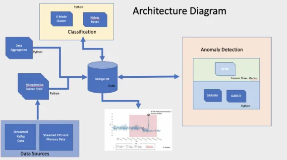
For this research log event, data will be captured. This data will come from a Kafka application log server. The data will be pulled every hour, parsed, cleansed, aggregated and fed into a Mongo database. Disk usage, CPU and memory information will be pulled hourly from a graphite server for the performance metrics. This data is already summarized so no aggregation will be necessary. For the initial exploratory analysis, a dashboard will be created and hosted on a local server. The dashboard will be made up of D3 time series charts. These charts will be near real-time as they will be fed from the automatic pushes of the aggregated data pulls. All code will be developed in python. For LSTM modelling the model will be implemented on Keras which sits on top of Tensor flow through the python Jupyter notebook. An architectural diagram of the platform is shown in figure 3.1
Figure 3.1: Anomaly Detection Architectural Diagram
3.1
Feature Identification
Kafka application log data was analysed. Exploration of the data concluded that there were only three types of log levels active on the server. Those were info, error and warn. No other log level severity type like debug or trace was found within the logs. For the performance metrics memory_percent_free and cpu_pct.use variables were identified. Features identified: • Info • Error • Warn • memory_percent_free • cpu_pct.use
• Timestamp
3.2
Data Cleansing
Data parsing will be done on the textual log messages to parse out the timestamp and severity type. Deeper parsing of the textual message itself will be conducted to bring back only the first 100 characters. For data cleansing, any row with no timestamp starting with 2018 or 2019 within the first set of characters will be removed from the dataset. All words will be converted to lower case. All stop words, punctuations, white spaces and numbers will be removed from the data set.
3.3
Missing Data
Initial observations identified that 66 individual hours of data was missing which equates to 2.75 days of data. The missing data occurred around the same time in-terval and was not widely dispersed throughout the data set. No imputation was implemented for this missing data. This missing data were included in the analysis for daily exploration but was excluded for hourly.
Exploratory Analysis
An exploratory analysis was first conducted on daily data. The data analysed was from 21/12/2018 - 26/02/2019. Hourly data from 01/01/2019 - 13/04/2019 was then analysed and used for the remainder of the research objectives as specified in chapter 2.
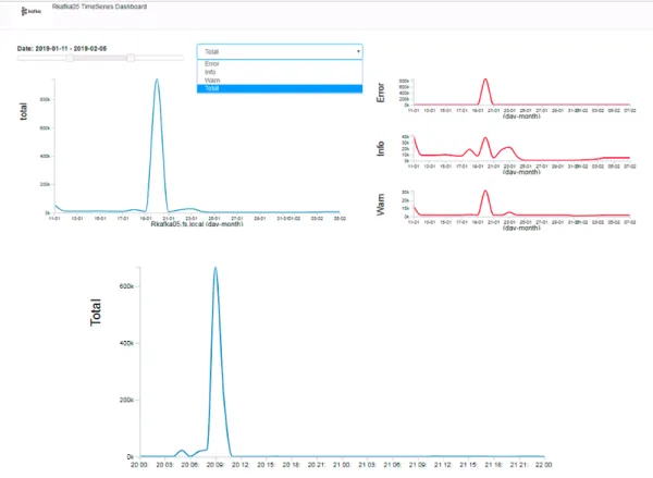
Figure 4.1 shows the time series dashboard that was created. It is used to visually inspect if there is any correlation between any of the different event type messages. The dashboard has been filtered to show a subset of the data from 11th January to 5th February because the 20th of January was the highest producer of log message events during the initial exploratory analysis phase.
Figure 4.1: Exploratory Analysis Dashboard
4.1
Daily Analysis
For the initial two months of the data table, 4.1 shows that a total of 1.5 million event type messages were produced. Out of those messages the error type events produced the highest number of events equating to a total of 55.5%.
Total Percent Total 1,574,682 100%
Info 560,828 35.62%
Error 874,336 55.52%
Warn 139,518 8.86%
For any analysis herein the alpha will be 0.05
4.1.1
Normality
Distribution analysis was done for each of the severity type messages. The first graph to the left in figure 4.2 shows info type messages not being of a normal distribution. The graph displays a platykurtic kurtosis with positive right-tailed skewness. Its quantile plot underneath it does confirm that the data is not normally distributed but does observe some fitting on the regression line. We also observe some outliers in the data. The middle and right graphs which show the warn and error distributions indicate a very volatile dataset due to the high volume of low counts of messages and a small volume of high count messages. The three quantile plots show that the data is not of a normal distribution for each of the severity type events.
Figure 4.2: Info, Warn, Error Daily Distribution Analysis
Figure 4.3: Daily Quantile Plots
For data to be of normal distribution its skewness should be zero and its kurtosis should be three. As per table 4.8 info, warn and error do not conform to the skewness and kurtosis values to be of a normal distribution.
Skewness Kurtosis
Info 2.5 9.1
Warn 6.7 48.7
Error 34.7 1261
Table 4.2: Daily Skewness-Kurtosis
SW and AD normalcy goodness of fit tests were conducted on the data.
Log Type Test Test Statistic P Value Info SW 0.7 0.0 AD 3.2 1.0 Warn SW 0.1 3.2 AD 21.6 1.0 Error SW 0.0 0.0 AD 585.9 1.0
Table 4.3: Daily Goodness Of Fit Tests
SW Test
Null Hypothesis: The data is normally distributed.
Alternative Hypothesis: The data is not normally distributed.
If p-value < 0.05 reject the null hypothesis. The data is not normally distributed.
AD Test
Null Hypothesis : The data is normally distributed.
Critical values [10%: 0.62, 5% : 0.74, 1% : 1.03]
If test statistic > critical values : Reject the null hypothesis the data is not normally distributed.
Normalcy Results Info :
We reject the null hypothesis of the SW test p=0.0. There is statistical evidence to suggest the data is not of a normal distribution. With the AD test (test statistic =3.2 > 5% at 0.74) we reject the null hypothesis. The data is not normally distributed.
Warn :
We fail to reject the null hypothesis of the SW test p=3.2. The AD test (test statistic =21.6 > 5% at 0.74) is showing strong evidence to suggest that the data is not nor-mally distributed.
Error :
We reject the null hypothesis of the SW test p=0.0. There is statistical evidence to suggest the data is not of a normal distribution. The AD test (test statistic =585.9 > 5% at 0.74) is showing strong evidence to suggest that the data is not normally distributed.
4.1.2
Unit Root Tests
Unit Root tests were conducted.
ADF
Null Hypothesis : Data has unit root (implies not stationary) Critical Values : [10%: -2.59, 5%: -2.90, 1%: -3.53]
If test statistic < critical values. Fail to reject the null hypothesis the time series has unit root and is not stationary.
KPSS
Null hypothesis : The data is stationary and does not have unit root. KPSS critical Values : [10% : 0.34, 5% : 0.46, 1% : 0.73]
If test statistic < critical value : Fail to reject the null hypothesis. The data does not contain unit root and is stationary.
Critical values for all tests:
ADF Critical Values : [10% : -2.59, 5% : -2.90, 1% : -3.53, ] KPSS Critical Values : [10% : 0.34, 5% : 0.46, 1% : 0.73]
Test Statistic P Value
ADF -2.21 0.20
KPSS 0.38 0.08
Table 4.4: Daily Info Unit Root Values
Test Statistic P Value
ADF -8.15 0.00
KPSS 0.12 0.10
Table 4.5: Daily Warn Unit Root Values
Test Statistic P Value
ADF -8.06 0.00
KPSS 0.1 0.10
Results: Unit Root Tests Info :
In the ADF test (p=0.20, test statistic (-2.21) < critical value (-2.90)). We accept the null hypothesis. The time series has unit root and is not stationary. For the KPSS test (test statistic (0.38) < critical value (0.46)) therefore we fail to reject the null hypothesis, the data is stationary.
Warn :
We reject the the null hypothesis for the ADF test (p=0.00, test statistic (-8.15) > critical value (-2.90)). The time series has no unit root and is stationary. For the KPSS test (test statistic (0.12) < critical value (0.46)). We fail to reject the null hypothesis the time series is stationary.
Error :
We reject the the null hypothesis of the ADF test (p = 0.00, test statistic (-8.06) > critical value (-2.90). The time series has no unit root and is stationary. We fail to reject the null hypothesis for the KPSS test (test statistic (0.1) < critical value (0.46)). Which implies the time series is stationary.
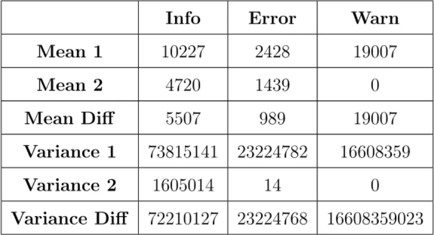
Mean and Variance Analysis
For forecast analysis, the data needs to be stationary in mean and variance for it to fit an ARIMA Model. The data was split into 2 random samples. Mean and variance tests were conducted on both samples.
Info Error Warn Mean 1 10227 2428 19007 Mean 2 4720 1439 0 Mean Diff 5507 989 19007 Variance 1 73815141 23224782 16608359 Variance 2 1605014 14 0 Variance Diff 72210127 23224768 16608359023 Table 4.7: Daily Mean-Variance Analysis
Table 4.7 shows that the data is not stationary in mean and variance as there are significant differences in mean on both samples for each severity type message. This is the same for the variance test.
4.1.3
Seasonality & Trends
Trend and seasonal graphs were created for info, warn and error type events. STL decomposition was done with the frequency set to weekly using the additive model. A monthly period was ignored due to the lack of initial data for analysis.
Figure 4.4: Daily Seasonal Decomposition Analysis
As per table 4.4 we visually observe that trend and seasonality do exist in the dataset. The graphs are displayed in order of observed, trend, seasonality and residuals. The trend is shown in the 2nd graph of the grouped graphs. For trend info type events
do show a variance change while warn events to show a transient type change and error events show the same as warn but not as apparent. Seasonality is shown in the third row of the grouped graphs and there does seem to be a repeat pattern over the time series. These patterns become more apparent when higher levels of frequency are used. A correlogram was also created to identify trends in the dataset.
Auto correlation - Partial Autocorrelation
Figure 4.5: Daily ACF PACF
For the correlogram, the first fifty lags were used. This gave fifty data points within the time-series to be tested for correlation and trends. We observe from the Info cor-relation chart that Info type events do show trend in the dataset while warn and error do not show any trends.
A statistical CH test was conducted to see if the data contained seasonality with the results concluding that there was no evidence of seasonality or trends in the dataset. An ARIMA difference utility test using ndiff was implemented to see how many times
we difference the data to remove trend. The result of the test indicated that there was no trend in the data set for any of the different types of severity messages. As such we conclude that there is no statistical evidence to suggest seasonality or trend exist but this may be taken with caution due to the graphical evidence presented.
4.1.4
Correlation
Pearson’s correlation analysis was implemented on the daily data to see if any of the event types have any type of relationship with each other. It is observed from figure 4.6 that info type events have a very strong correlation with warn events (0.7). Info events also have a strong correlation with error events (0.5). Error and warn events do show a significant correlation with each other of (0.9). The results of the Pearson’s test conclude that there is strong statistical evidence of relationships between each of the different event types.
4.2
Hourly Analysis
The hourly analysis was conducted on the event type data.
4.2.1
Normality
Histograms and quantile plots were graphed on the hourly data to indicate as to the data’s distribution and shape.
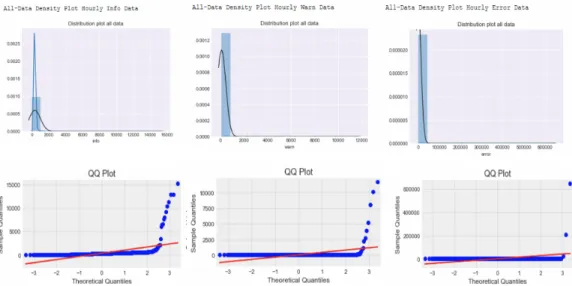
Figure 4.7: Hourly Distribution Analysis
Figure 4.7 shows that the data does not conform to a normal distribution as the data is not a symmetrical shape on the histograms and does not fit along the regression lines in the quantile plots. The histograms also show that the data is contained within a small range of values.
As per table 4.8 info, error and warn do not conform to the skewness and kurtosis tests to be of a normal distribution.
Skewness Kurtosis
Info 215.4 272.0
Warn 25.1 680.9
Error 45.2 2144.2 Table 4.8: Hourly Skewness - Kurtosis
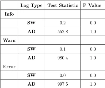
Normalcy goodness of fit tests was conducted on the data. SW and AD tests were implemented.
Log Type Test Statistic P Value Info SW 0.2 0.0 AD 552.8 1.0 Warn SW 0.1 0.0 AD 980.4 1.0 Error SW 0.0 0.0 AD 997.5 1.0
Table 4.9: Hourly Goodness Of Fit Tests
SW Test
Null Hypothesis: The data is normally distributed.
If p-value < 0.05 reject the null hypothesis. The data is not normally distributed.
AD Test
Null Hypothesis : The data is normally distributed. Critical values [10% : 0.65, 5% : 0.78, 1% : 1.09]
If test statistic > critical values : Reject the null hypothesis the data is not normally distributed
Info, warn and error event types reject the null hypothesis for the AD test. The data is not normally distributed. The SW test also rejects the null hypothesis, the data is not normally distributed.
4.2.2
Stationarity
The stationarity tests that were implemented on the hourly data.
ADF Test
Null Hypothesis: Data has unit root(implies not stationary). Critical values: [10% : -2.56, 5% : -2.86, 1% : -3.43]
P value < 0.05: Reject the null hypothesis, the data is stationary.
If ADF statistic > critical values: Reject the null hypothesis of unit root. The time series is stationary.
KPSS Test
Null hypothesis for the KPSS test : The data is stationary Critical values: [10%: 0.34, 5% 0.46, 1%: 0.73]
If test statistic < critical value : Fail to reject the null hypothesis, the data is stationary.
ADF critical values: [10% : -2.56, 5% : -2.86, 1% : -3.43] KPSS critical values: [10%: 0.34, 5% 0.46, 1%: 0.73]
Test Statistic P Value
ADF -19.27 0.00
KPSS 1.28 0.01
Table 4.10: Hourly Info Stationarity Values
Test Statistic P Value
ADF -13.49 0.00
KPSS 0.27 0.1
Table 4.11: Hourly Warn Stationarity Values
Test Statistic P Value
ADF -27.00 0.00
KPSS -0.13 0.1
Table 4.12: Hourly Error Stationarity Values
Results: Unit Root Tests
The time series is stationary for info and error type events as they pass both the KPSS and ADF test. Warn type events do pass the ADF test but fail the KPSS test.
4.2.3
Seasonality & Trend
A trend and seasonality graph was created. The graph was based on hourly data. As per table 4.8 it is visually observed that there was a negative followed by a positive trend detected in the monthly time series data for info event types. A step downward type trend was detected for warn and error type events. Seasonality is observed for each severity event type.
A statistical CH test was conducted to see if the data contained seasonality. The test was implemented for daily, weekly and monthly frequencies. The results conclude that there is no evidence of seasonality in the dataset for daily and weekly data but there was evidence of seasonality in monthly data for info and warn but none for error.
4.2.4
Correlation
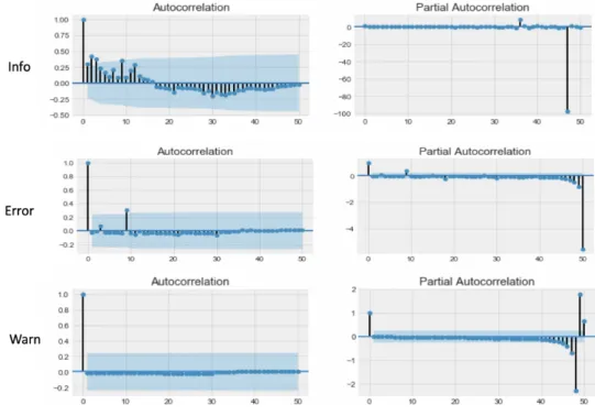
ACF-PACF
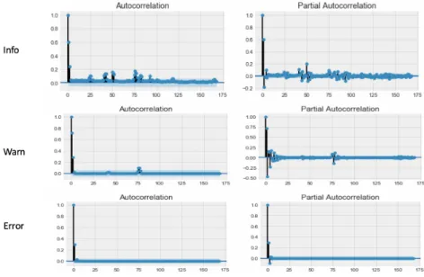
Figure 4.9: Hourly ACF-PACF
For the correlation chart in figure 4.9 , the first 168 lags were used. This is a representa-tion of one week’s worth of time series data. We observe from the info correlarepresenta-tion chart that there is still some correlation within the time series data around lag twenty-five
onwards which is an indication that the time series data is dependant on its previous time series observations. The partial autocorrelation chart shows that there is still some residual noise which exceeds the significance threshold. For warn, there appears to be no correlation on the data except for the first three lags with the PACF still showing some residuals on the first ten lags. For error, there was no correlation at all through the time series except around lag two. Looking at the p and q values for ARIMA modelling
Info: The data would need to be differenced to become more stationary
Warn: The data would need to be differences to get rid of the residual noise on the PACF plot
Error : (1,1)
We conclude from the hourly data that transformation should be implemented on info and warn and no transformation is required for error data.
4.2.5
Cross Correlation
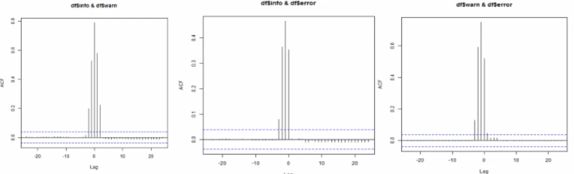
Hourly cross-correlation analysis was done on all the different event types. The lag value was set to twenty-four which represents a full day. Cross-Correlation was con-ducted on all untransformed events.
Figure 4.10: Hourly Cross Correlation
The results of the cross-correlation charts imply that info and warn have a significant correlation at lag one and lag two. This implies that an info event will become a warn
type event within the first two lags which represents the t-1 with a less significant correlation at t-2. The info and error correlation chart have significant correlation at lag one. This implies that an Info type event does have a strong correlation with an error type event at t-1. The warn and error correlation chart also show significant correlation at lag one. This implies that a warn type event will result in an error type event within the first hour as the time will be t-1.
Time Series Modelling
5.1
GARCH
A GARCH Model was implemented on each of the non transformed and transformed datasets so that an LM test could be conducted. The result of the LM test was to conclude if heteroscedasticity occurred in the model and if so it implied that the data was volatile and not suitable for ARIMA modelling.
LM Test Results On Non-Transformed Data
Test Statistic P Value
Info -4.37 0.99
Warn 0.02 1.00
Error 11.03 0.27
Table 5.1: Hourly Engle’s LM Test for Autoregressive Conditional Heteroscedastici