Amodal Instance Segmentation and Multi-Object Tracking with Deep Pixel Embedding

(1)

DigitalCommons@University of Nebraska - Lincoln

Theses, Dissertations, and Student Research

from Electrical & Computer Engineering Electrical & Computer Engineering, Department of Fall 12-5-2019

Amodal Instance Segmentation and Multi-Object Tracking with

Deep Pixel Embedding

Yanfeng Liu

University of Nebraska - Lincoln, [email protected]

Follow this and additional works at: https://digitalcommons.unl.edu/elecengtheses

Part of the Computer Engineering Commons, and the Other Electrical and Computer Engineering Commons

Liu, Yanfeng, "Amodal Instance Segmentation and Multi-Object Tracking with Deep Pixel Embedding" (2019). Theses, Dissertations, and Student Research from Electrical & Computer Engineering. 111.

https://digitalcommons.unl.edu/elecengtheses/111

This Article is brought to you for free and open access by the Electrical & Computer Engineering, Department of at DigitalCommons@University of Nebraska - Lincoln. It has been accepted for inclusion in Theses, Dissertations, and Student Research from Electrical & Computer Engineering by an authorized administrator of

(2)

Yanfeng Liu

A THESIS

Presented to the Faculty of

The Graduate College at the University of Nebraska In Partial Fulfilment of Requirements

For the Degree of Master of Science

Major: Electrical Engineering

Under the Supervision of Professors Eric T. Psota and Lance C. P´erez

Lincoln, Nebraska

(3)

DEEP PIXEL EMBEDDING Yanfeng Liu, M.S. University of Nebraska, 2019

Advisor: Eric T. Psota and Lance C. P´erez

This thesis extends upon the representational output of semantic instance segmentation by explicitly including both visible and occluded parts. A fully convolutional network is trained to produce consistent pixel-level embedding across two layers such that, when clus-tered, the results convey the full spatial extent and depth ordering of each instance. Results demonstrate that the network can accurately estimate complete masks in the presence of occlusion and outperform leading top-down bounding-box approaches.

The model is further extended to produce consistent pixel-level embeddings across two consecutive image frames from a video to simultaneously perform amodal instance seg-mentation and multi-object tracking. No post-processing trackers or Hungarian Algorithm is needed to perform multi-object tracking. The advantages and disadvantages of such a bounding-box-free approach are studied thoroughly. Experiments show that the pro-posed method outperforms the state-of-the-art bounding-box based approach on tracking animated moving objects.

(4)

graduate experience productive and enjoyable. I would like to extend my sincere thanks to Dr. Stephen Scott for being my committee member. I would like to thank the senior graduate students in my lab, Jay Carlson and Mateusz Mittek, for their encouragement and discussions about research ideas. Finally, I would like to thank my family and friends who have always supported me throughout my time at the University – none of this would have been possible without them.

(5)

http://bit.ly/34Xjuvm . . . 15 7 Sample instance segmentation result from Mask R-CNN [4] . . . 16 8 Intersection over union. Image frombit.ly/33RC9Yq. . . 17 9 The effect of non-max suppression. Image frombit.ly/2YjNe38 . . . 17 10 A failure case of non-max suppression. Image frombit.ly/355TkXi . 18 11 Optical flow, tracked through multiple frames and visualized on the last

frame. Image fromhttp://bit.ly/2PjjDTk . . . 19 12 Human key-points estimation [5] . . . 19 13 Structure from motion. Image fromhttp://bit.ly/2YjQsUk . . . . 20 14 Stereo Matching. Top: left and right view. Bottom: color-coded depth map

and 3D reconstructed scene. Image fromhttp://bit.ly/2LoAfrS. . 21 15 A generic architecture of fully connected networks. Image rendered by

http://bit.ly/2s28oa8 . . . 23 16 Plot of various activation functions. Image rendered by the author. . . 25 17 Process of a convolutional filter convolving with the input. Note how

the output location corresponds to the location of the input. Image from http://bit.ly/2PkeSsz . . . 26

(7)

18 Procedure of Stochastic Gradient Descent. Image from http://bit.

ly/2PkLSRP . . . 27

19 A generic architecture of recurrent neural networks. Image fromhttp: //bit.ly/2rUkou5 . . . 30

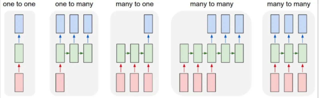
20 Flexible input/output for recurrent neural networks. Image from http: //bit.ly/2LqwsKw . . . 30

21 Architecture of LSTM recurrent neural networks. Image from http:// bit.ly/2rUkou5 . . . 31

22 Sample data from MNIST dataset [6] . . . 33

23 Sample data from ImageNet dataset [7] . . . 33

24 Workflow diagram for VAE. Image fromhttp://bit.ly/2PkLS4b . . 34

25 Results of continuous sampling from VAE. Image from http://bit. ly/2YkLeaQ . . . 36

26 Workflow diagram for GAN. Image fromhttp://bit.ly/2YnloCZ . 37 27 GauGAN. Note how the reflection matches the shape of the mountain and the color of the sky [8] . . . 39

28 Image In-Painting. (a) shows the processing of masking void areas; (b) shows the completed mask and repaired image [9] . . . 39

29 Realistic images generated by BigGAN [10]. Yes they are all fake. . . 40

30 Connection in ResNet [11] . . . 40

31 Connection in DenseNet [12] . . . 41

32 Connection in randomly wired neural networks [13] . . . 42

33 Architecture of SegNet [14] . . . 43

(8)

instance segmentation. . . 45

36 DYCE [16] image and ground truth mask for “wall”; it appears that the mask for light reflected off the wall is provided instead . . . 47

37 KINS [17] . . . 48

38 SAIL-VOS [18] . . . 49

39 MOT workflow [19] . . . 53

40 Instance segmentation output scenarios for two overlapping rectangles. Im-age rendered by the author. . . 59

41 Sample training data. From left to right: input image, foreground class mask, occlusion class mask, foreground instance mask, occlusion instance mask. . . 61

42 Proposed segmentation architecture. . . 62

43 Performance for different number of instances per class and different em-bedding dimensions C. x-axis is number of instances, y-axis is different metrics, and colored lines represent models with differentC. . . 65

44 Failure cases for embedding model. Red circle indicates a triple stack. . . . 66

45 First failure case for Mask R-CNN. Left to right: ground truth, unfiltered proposals, filtered proposals . . . 67

46 Second failure case for Mask R-CNN. Left to right: ground truth, filtered proposals, final results . . . 67

47 Sample results from the segmentation embedding model. From left to right: image, embedding, embedding masked by semantic segmentation, instance clustering, instance ground truth, semantic segmentation predic-tion, semantic segmentation ground truth . . . 69

(9)

48 Identity switches to the other object that also appears in the same bounding

box. Image from [20] . . . 71

49 Issues with bounding boxes compared to masks. Image from [21] . . . 72

50 Proposed tracking architecture. . . 74

51 Sample sequence of moving shapes dataset . . . 75

52 Multi-frame tracking process . . . 77

53 Architecture of JDE [20] . . . 78

54 Sample results of the JDE embedding model on difference sequences. . . . 81

55 Sample results from the MOT embedding model. From left to right: image pair, masked foreground embedding and background embedding for image pair, foreground and background instance clustering for image pair . . . 82

56 Sequence 1 of tracking results produced by our MOT embedding model . . 83

57 Sequence 2 of tracking results produced by our MOT embedding model . . 84

58 Qualitative results of the embedding based tracking model on rotate shapes, sequence 1. . . 85

59 Qualitative results of the embedding based tracking model on rotate shapes, sequence 2. . . 86

(10)

2 Performance of models on 6 instances per class with different NMS thresh-oldt . . . 64 3 Performance of models on 12 instances per class with different NMS

thresh-oldt . . . 64 4 Performance of instance masks constructed from different number of layers

of ground truth masks. N is the number of instances per class. . . 68 5 Performance of our proposed embedding model and the JDE model on 5

(11)

1 Introduction

Computer vision is a field that focuses on a high-level algorithmic understanding of digital images. It strives to intelligently describe everything in an image, such as the localiza-tion/classification/action of an object, the relationship between objects, and the 3D struc-ture of the scene. Since videos can be treated as a collection of images, they are included in the consideration of computer vision. With videos, more complex spatiotemporal tasks emerge, such as the re-identification of the same objects across multiple images, multi-object tracking, structure from motion, and odometry estimation.

The field of computer vision has gained increasing popularity after the huge success of deep learning since AlexNet was proposed in 2012 [1]. Fig 1 shows the architecture of AlexNet. Back then GPUs (Graphics Processing Unit) were not optimized for neural networks yet and AlexNet was too big to fit on one GPU so it was distributed to multiple GPUs. The applications of deep learning have now flourished in many domains, such as object detection [4] and tracking [22], semantic segmentation [23], instance segmentation [24], image synthesis [25], and video synthesis [26].

Deep learning is a sub-field of machine learning that utilizes the effective modeling ca-pability of deep neural networks in many tasks, including computer vision, natural language understanding, reinforcement learning, etc. It serves as a powerful tool that automates

(12)

back-propagation. The network is expected to gradually formalize filters that are capable of modelling increasingly complex relationships as the number of layers and weights go up.

Before deep learning, a lot of algorithms were elaborately and manually designed by re-searchers. It was a very time-consuming process and often limited to specific environments and applications. The features extracted from human-designed algorithms have both the blessing and the curse of interpretability. On one hand, people understand exactly what the features are trying to capture, but, on the other hand, there could be untapped features that are potentially useful but not directly understandable to human beings. In overly complex problems, it is also unclear how to capture the correct features needed for a generalized solution. Deep learning, in contrast, is a one-size-for-all solution that learns features in an iterative process. Researchers now instead focus on the problem formulation and weight optimization aspects of the problem-solving.

In general, there are three classes of learning paradigms in machine learning: super-vised learning, semi-supersuper-vised learning, and unsupersuper-vised learning. In supersuper-vised learn-ing, every training example is presented as a pair of input and expected output, or ground truth; in semi-supervised learning, a small set of labelled data and a larger set of unlabelled data are provided; in unsupervised learning, the input is provided without the ground truth, which should be instead inferred from the input itself.

Deep learning thrives in all three learning paradigms. Most vision tasks mentioned above can be formulated as any of the three paradigms. Classic supervised learning is the most obvious route, but it requires a lot of human effort to provide the labelled data. When labelled data is too expensive or impractical to obtain due to the limitations of human labor, it often becomes the bottleneck of the performance. Semi-supervised learning has

(13)

shown promising results where the model learns useful feature extraction from unlabelled data through techniques such as auto-encoding [27] before fine-tuning on labelled data. Unsupervised learning is the most challenging to design but also the most promising. Once formulated, an unsupervised model can essentially use cheaply obtained training data and benefit from a diverse set of data distributions.

Given the advancement in tools and algorithms in recent years, computer vision re-searchers have become progressively more interested in a precise, pixel-wise understand-ing of images. From crude to precise, image understandunderstand-ing tasks can be ordered as: image classification – bounding box localization and classification – semantic segmentation – se-mantic instance segmentation – panoptic segmentation, each providing more information than the last.

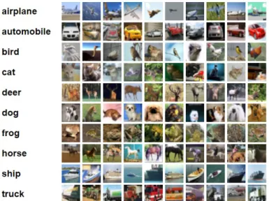
Image classification assigns a class label to an entire image. For example, if an image contains a truck as the salient object, it should be assigned the “truck” label regardless of its exact appearance or background. Figure 2 shows a classic dataset, CIFAR-10 [28], for image classification. In image classification, the challenge is to model the variety of a category of objects. For example, trucks should all have wheels and large space for cargo. In recent years, neural networks have achieved super-human performance (defined roughly as lower than 5.1% top-5 error rate) on certain datasets of image classification [11, 29], such as ImageNet [7].

Bounding box localization and classification, also known as object detection, takes im-age classification one step further. Its goal is to produce the exact location of the object of interest. By drawing a bounding box around the object, it also opens up the possibility of labelling multiple objects at the same time. For example, in Figure 3, there are multiple human faces in the image. The algorithm draws a bounding box around each face and clas-sifies it as “face.” Object detection is an active research area with the support from large datasets such as Microsoft COCO, PASCAL, and Labeled Faces in the Wild [30, 31, 32]. Object detectors generally fall into two categories, one-stage detectors such as [33, 34],

(14)

Figure 2: Image classification from CIFAR-10. Image from http://bit.ly/ 33Mspyw

and two-state detectors such as [35, 36, 37]. The difference is one-stage detectors output a fixed number of detections on a grid while two-stage detectors propose an arbitrary number bounding boxes and filter them in post-processing.

Figure 3: Face detection on multiple people [2]

Semantic segmentation takes image understanding to another level by assigning a class label to each pixel, achieving localization and classification at the finest granularity. For example, in Figure 4, the algorithm labels each pixel that belongs to the “person” class as red, drivable road as purple, sidewalk as pink, road signs as yellow, and street lights as orange. The actual colors do not matter as long as they are consistent for the same class. Modern semantic segmentation methods mostly rely on fully-convolutional neural

(15)

networks [15, 14]. Datasets like CityScape and KITTI [3, 38] provide large amounts of driver-view training data, mostly for autonomous driving research purposes.

Figure 4: Semantic segmentation on a street view in the CityScape dataset [3]

Instance segmentation looks beyond the semantic classification of the pixel and assigns a unique identity to each visible object within the same class. For example, in Figure 5, the pixels that belong to chairs are correctly identified and separated from all other objects in the scene, plus each chair has a distinct identity (illustrated with a unique color) consistent within its boundary. Some methods build on top of object detection and estimates the object mask within the bounding box [4, 39, 40], while the others take a bottom-up approach that assigns properties to pixels and cluster them later into instance masks [41, 42, 43].

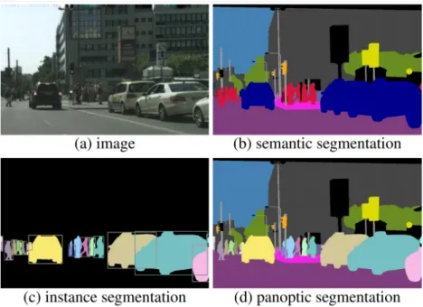
Panoptic segmentation combines semantic segmentation and instance segmentation into one task. The countable things are treated as instances where as the uncountable “stuff” is treated as semantic segmentation. It aims to assign a class and/or identity to every pixel in the image. It was first proposed by Alexander Kirillov et al. in 2018 [44], which also

Figure 5: Semantic instance segmentation on chairs. Image from http://bit.ly/ 2DRMRTW

(16)

Figure 6: A side-by-side comparison of different segmentation tasks. Image fromhttp: //bit.ly/34Xjuvm

introduced a new Microsoft COCO Panoptic dataset for the task. Others quickly followed up on improvements [45, 46, 47, 48, 49]. Figure 6 compares the relationship between semantic segmentation, instance segmentation, and panoptic segmentation.

Even though panoptic segmentation provides classification and identity for each pixel in the image, it is by no means the end of all pixel-level tasks. So far the focus has been on the visible portion of the image, but human beings have much stronger perceptive capability in the sense that they are also able to infer what is occluded. We don’t simply assume an object is cut in half just because we can only see half of it. We imagine where the rest of it is and what it looks like based on what we see. Amodal segmentation fulfills this need by explicitly estimating the complete mask based on the visible part. This is particularly useful in tasks such as multi-object detection and tracking because, ideally, objects should not be lost when briefly occluded.

Instance segmentation, either modal or amodal, traditionally has two general branches of techniques, top-down and bottom-up, as mentioned previously. The top-down approach, much like a two-state object detector, relies heavily on generating bounding boxes around

(17)

objects. The instance mask is then estimated strictly within the boundary of the box, as shown in Figure 7.

Figure 7: Sample instance segmentation result from Mask R-CNN [4]

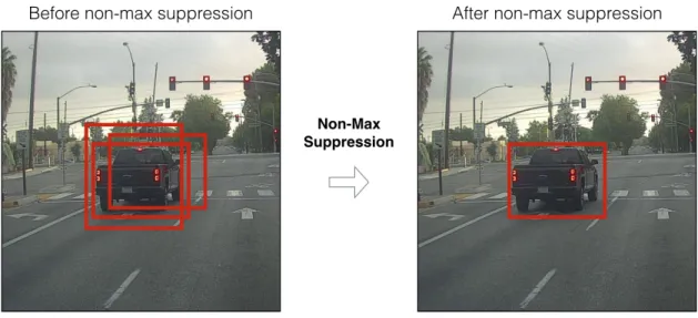
In cluttered scenes where a lot of objects are overlapping, it becomes challenging to generate bounding boxes for each object due to non-maximum suppression (NMS). NMS is a necessary step to filter out overlapping bounding boxes. It achieves this filtering typ-ically by calculating the intersection over union (IOU) between candidate boxes. IOU is designed to measure the extent of overlapping between two shapes. NMS sorts all bound-ing boxes by their confidence scores. When two boxes have an IOU over a pre-determined threshold, NMS discards the one with a lower confidence score and keeps the other. Figure 8 illustrates the definition of IOU.

Current bounding box proposal methods typically generate many more boxes than the actual number of objects, in the hopes that a post-processing algorithm will only keep the candidates that have both the highest confidence and the best overall fit for each object. Figure 9 demonstrates the effect of such post-processing. The problem with this approach is that, when objects are cluttered and overlapping, a lot of valid bounding boxes are treated

(18)

Figure 8: Intersection over union. Image frombit.ly/33RC9Yq

as false-positives and discarded. Figure 10 shows such a failure case. Several modifica-tions such as Soft NMS and Softer NMS are proposed to mitigate this issue [50, 51]. They improve benchmark scores but do not address the fundamental problem of bounding boxes – bounding boxes can repeatedly cover the same region multiple times and they intention-ally do so to systematicintention-ally cover important visual clues. Methods like [35] even explicitly allow ~2k bounding box proposals in the intermediate step to cover the image as much as possible. As long as bounding boxes are still part of the algorithm, this problem will persist.

Figure 9: The effect of non-max suppression. Image frombit.ly/2YjNe38

(19)

Figure 10: A failure case of non-max suppression. Image frombit.ly/355TkXi

for the salient object of the detected class and two objects are both visible in the bounding box, it can be confusing to decide which one is the targeted object. Technically, both of them are, so the algorithm ends up attempting to cover both objects with a strange shape. Examples of this type of error are shown in later chapters.

Other than the tasks mentioned above, there are other areas in computer vision that take advantage of videos instead of static images. Videos consist of multiple frames of highly correlated content. The fact that neighboring frames are taken within temporal and spatial proximity provides extra information.

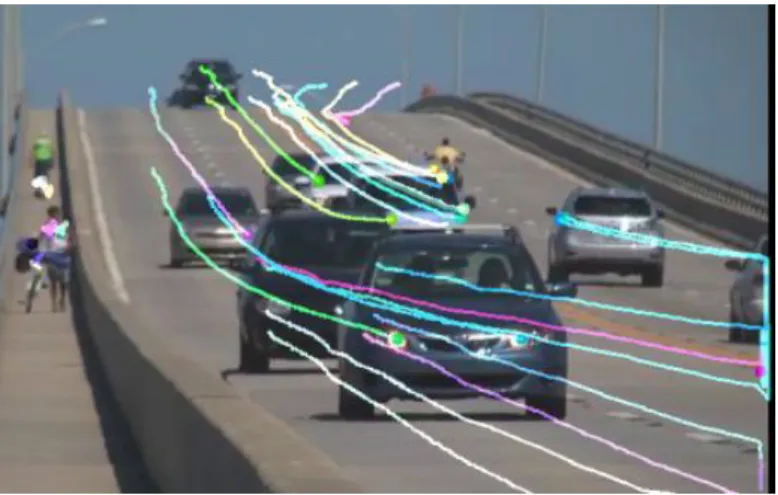
Optical flow is usually calculated to visualize pixel movement between consecutive video frames and help track object movement, as shown in Figure 11. Traditionally this is done through a differential method called the Lucas-Kanade method [52, 53]. Modern methods rely heavily on deep learning to estimate optical flow through either supervised learning [54, 55] or unsupervised learning [56]. Optical flow can also be jointly learned with other tasks such as depth estimation [57] and segmentation [58].

Human key-points estimation is usually done jointly with human detection [4] to pro-vide extra information to be used in pose estimation [59, 60] or fun applications such as synthesized dancing videos [61] or motion capture. Figure 12 demonstrates the task of

(20)

Figure 11: Optical flow, tracked through multiple frames and visualized on the last frame.

Image fromhttp://bit.ly/2PjjDTk

Figure 12: Human key-points estimation [5]

human key-points estimation.

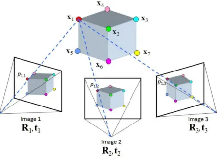
Three dimensional reconstruction is another area that leverages the power of videos. The concept is that a camera moves continuously in a 3D space, taking 2D images peri-odically. The appearances of objects warp based on their shape and distant to the camera. Structure from motion extracts feature points from frames and re-projects them into the 3D scene in order to reproduce the structure [62]. Stereo matching tackles the problems differ-ently. Stereo matching assumes that two cameras are side-by-side and calculates the depth at every pixel by measuring how much each pair of corresponding pixels shifts between the left and right image [63]. Figure 13 and 14 illustrate the two methods.

Among current research areas mentioned above, amodal instance segmentation and multi-object tracking are the two areas that strive for the highest level of scene

(21)

understand-ing. One describes the complete shapes of objects regardless of their visibility, the other preserves the identities of multiple objects, given their detections, across video frames. This thesis focuses on these two areas and proposes a unified method for both. The pro-posed method is intuitive yet powerful. It is easy to construct, with very few parameters to manually tune. Specifically, the contributions of this thesis include:

• Investigate the limitations of bounding boxes in highly crowded scenes for both in-stance segmentation and tracking;

• Propose a bounding-box-free method for amodal instance segmentation based on pixel embeddings;

• Extend the proposed method into a multi-object tracking method without motion modelling or complex identity matching post-processing;

• Compare the behaviors and trade-off between the proposed models and state-of-the-art models in the literature to highlight current issues in segmentation and tracking.

(22)

Figure 14: Stereo Matching. Top: left and right view. Bottom: color-coded depth map and 3D reconstructed scene. Image fromhttp://bit.ly/2LoAfrS

(23)

2 Related Work

2.1 Deep Learning and Computer Vision

2.1.1 Components of Deep Learning

Even though the new wave of deep learning interest only started in 2010s, the core compo-nents and fundamentals of deep learning are not young. This section reviews the develop-ment of deep learning from the last century and introduces the core concepts and techniques along with their history.

The foundational concept of perceptron [64] was first introduced in 1957. Frank Rosen-blatt proposed it as a binary classification algorithm that has the following rule:

f(x) =        1 ifw·x+b >0, 0 otherwise (1)

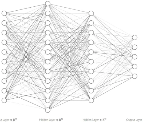
wherewandxare vectors of real values of the same length, and b is the bias. Today, the form ofw·x+bis still a fundamental computing rule in a fully connected network. The difference is that neural networks now are much more flexible than simple binary classifi-cation. Eachf(x)and the non-linear activation function after it are together considered a “neuron”. A generic architecture for fully connected neural networks is shown in Figure 15. In this case, the network has one input layer, two hidden layers, and an output layer. The dimensions of inputs and outputs are pre-defined by the problem, but there is a lot of flexibility for how many hidden layers and how many neurons per layer a network can have. Generally, the capacity of network increases as the network gets more complicated.

What is not shown in Figure 15 is the activation function. There is an activation function for every layer of the neural network. The function can have many designs to choose from, but it needs to be differentiable and nonlinear. The differentiability allows backpropagation, thus training, of the neural network. The nonlinearity provides the network with the ability

(24)

Figure 15: A generic architecture of fully connected networks. Image rendered byhttp: //bit.ly/2s28oa8

to model nonlinear relationships in data, which is what makes neural networks powerful. If there is no nonlinear activation function, then the entire fully connected network can be reduced to one matrix multiplication. In other words, there is no reason to have multiple layers without nonlinear activation functions.

Consider a two-layer fully connected network without activation functions. It can be represented as

f(x) = A1(A0x+b0) +b1,

which can be simplified as

(25)

LetA =A1A0andb=A1b0+b1, then we have

f(x) = Ax+b ,

which is the form of a one-layer fully connected network.

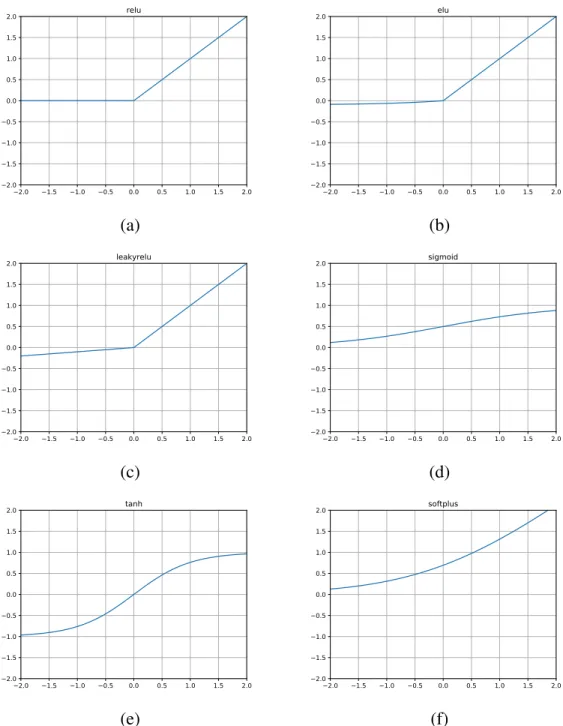
Common choices of nonlinear activation functions include ReLU (Rectified Linear Unit) [65], LeakyReLU [66], ELU (Exponential Linear Unit) [67], Sigmoid, Hyperbolic Tangent (tanh), and softplus [68]. Figure 16 shows each function listed above. Their equa-tions are as the following:

ReLU(x) =        x ifx >0, 0 otherwise , ELU(x) =        x ifx >0, α(ex₋₁₎ _otherwise , LeakyReLU(x) =        x ifx >0, αx otherwise , Sigmoid(x) = 1 1 +e(₋_x₎, tanh(x) = e x₋_e−x ex₊_e−x , softplus(x) = ln(1 +ex).

Fully connected networks work well with one dimensional data, sometimes two dimen-sional data if it is flattened to be one-dimendimen-sional but, in general, fully connected networks struggle to work well on two dimensions and beyond due to its input format limitations. By design, the input of a fully connected network is a one-dimensional vector of fixed size. Inputs of different shapes have to be cropped or padded, depending on whether they have more numbers or fewer. In contrast, convolutional neural networks solve this problem by

(26)

2.0 1.5 1.0 0.5 0.0 0.5 1.0 1.5 2.0 2.0 1.5 1.0 0.5 0.0 0.5 1.0 1.5 2.0 relu 2.0 1.5 1.0 0.5 0.0 0.5 1.0 1.5 2.0 2.0 1.5 1.0 0.5 0.0 0.5 1.0 1.5 2.0 elu (a) (b) 2.0 1.5 1.0 0.5 0.0 0.5 1.0 1.5 2.0 2.0 1.5 1.0 0.5 0.0 0.5 1.0 1.5 2.0 leakyrelu 2.0 1.5 1.0 0.5 0.0 0.5 1.0 1.5 2.0 2.0 1.5 1.0 0.5 0.0 0.5 1.0 1.5 2.0 sigmoid (c) (d) 2.0 1.5 1.0 0.5 0.0 0.5 1.0 1.5 2.0 2.0 1.5 1.0 0.5 0.0 0.5 1.0 1.5 2.0 tanh 2.0 1.5 1.0 0.5 0.0 0.5 1.0 1.5 2.0 2.0 1.5 1.0 0.5 0.0 0.5 1.0 1.5 2.0 softplus (e) (f)

(27)

Figure 17: Process of a convolutional filter convolving with the input. Note how the out-put location corresponds to the location of the inout-put. Image from http://bit.ly/ 2PkeSsz

utilizing small convolutional filters to convolve with the input. The input can be one, two, three, or higher dimensional. The most commonly used are two and three dimensional convolution filters. They are usually of size (3×3), (5×5), or (7×7). Bigger sizes are theoretically possible but rarely used. The size of each spatial dimension also needs to be an odd number in order to preserve the shape of the input. Figure 17 demonstrates the process of a two dimensional convolution. At the borders of the input image, the designer of the algorithm has a choice between zero-padding the border or leaving it as-is. Zero-padding will cause the output of convolution to have the same shape as the input, whereas leaving it as-is will cause the output to have a smaller shape. In the case of Figure 17, there is no zero-padding, so the input image changes from5×5to3×3

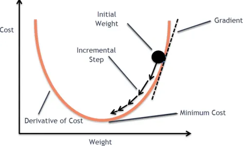
The convolutional layer has many variants. One of them is the atrous convolutional layer. It allows the layer to have explicit control over the output resolution by changing how “sparse” the atrous convolution filters are. Another variant is the convolution transpose layer. It increases the output resolution compared to the input in contrast to decreasing it in normal convolution layers. This is achieved by flipping the order of the input and the filter. To train a neural network, whether it is convolutional or fully connected, a core tech-nique called Stochastic Gradient Descent (SGD) was introduced. In 1951 and 1952, two

(28)

Figure 18: Procedure of Stochastic Gradient Descent. Image from http://bit.ly/ 2PkLSRP

papers were published that were considered the foundational works of SGD. It is an itera-tive optimization algorithm to minimize/maximize the value of a function. It works in the following stages: (1) start at a random location on the function value plane with random parameters; (2) find the gradient with respect to the parameters to decide the direction for its next step; (3) update by taking a step of predefined step size in that direction; (4) repeat step (2) and (3). Figure 18 shows the stages of SGD.

SGD requires the gradients of the function to be known. It is done through a technique called automatic differentiation (autodiff). In 1970, the earliest form of general automatic differentiation was developed by Seppo Linnainmaa [69, 70], even though it was not called “backpropagation” at the time. Modern deep learning frameworks use the reverse mode automatic differentiation for calculating gradients. The procedure is best shown through a toy example.

Assume we want to calculate the gradient for

(29)

with respect tox1, x2, x3 whereαandβare constants. In other words, we are interested in df dx1, df dx2, df

dx3. The algorithm breaksf down to basic units whose the gradient functions are

known and clearly defined. In this case,

y1 =x1x2,

y2 =x23,

y3 =αy1,

y4 =βy2,

y5 =y3+y4.

It then uses the commonly known Chain Rule to iteratively find the gradients with respect to the target parameters. As a reminder, the Chain Rule states that, if there are three variables

a, b, cwhere adepends band b depends onc, and we are interested in the derivative ofa

with respect toc, then it can be calculated as

da dc = da db · db dc.

In the case of the example, gradients for each intermediate step can be easily obtained as the following: dy5 dy3 = 1,dy5 dy4 = 1,dy3 dy1 =α,dy4 dy2 =β,dy1 dx1 =x2, dy1 dx2 =x1, dy2 dx3 = 2x3.

(30)

df dx2 = df dy3 · dy3 dy1 · dy1 dx2 = 1·α·x1, df dx3 = df dy4 · dy4 dy2 · dy2 dx3 = 1·β·2x3.

The exact values of these gradients can then be easily calculated when constant α, β

and the values ofx1, x2, x3are plugged in.

Many optimization algorithms proposed over the years. Among them, the most famous ones include Adamax [71], Adam [71, 72], RMSProp, AdaGrad [73], Adadelta [74], and Nadam [75]. They propose extensions on top of the original SGD by introducing ideas such as momentum, sliding window average of gradients, and adaptive learning rate. The choice of optimizer, together with learning rate, can be a deciding factor in machine learning. Therefore it should be carefully tested through a search algorithm.

In 1997, long-short term memory (LSTM) recurrent neural network was invented by Sepp Hochreiter and J¨urgen Schmidhuber [76]. LSTM is still one of the core modules in modern research of recurrent neural networks (RNN). To be able to appreciate LSTM, one first needs to understand the vanilla RNN design. RNNs are the backbone of natural lan-guage processing. They have the architectural advantage of being able to handle sequential data naturally. Language is one of the two manifestations of intelligence, together with visual understanding. Therefore, being able to understand human languages, translating them to one another, rephrasing with similar meanings attracted huge research interest in the community. Previously neural networks have been a state-less model, meaning that the content and ordering of previous inputs and outputs have no effect on the next inputs or outputs. Being able to retain information in a way that models human memory is desir-able in sequential data processing. The recurrent neural network was designed to solve this

(31)

Figure 19: A generic architecture of recurrent neural networks. Image from http:// bit.ly/2rUkou5

Figure 20: Flexible input/output for recurrent neural networks. Image from http:// bit.ly/2LqwsKw

particular problem. Figure 19 shows a generic architecture of a RNN.

In the figure, there is a hidden state, denoted as ht for time stept. The hidden state

is affected by the previous inputs so that it produces different outputs of the same input

xt+1 in time step t + 1 given different previous inputs from time step 0 to t. The right

hand side of the figure is the setup unrolled in time. This architecture is very flexible in its input/output arrangement. It can be one-to-one, one-to-many, to-one, many-to-many, with arbitrary input and output length. Figure 20 illustrates these input/output arrangements.

The computation of RNN is as follows. Let xtbe input at timet,ht be hidden state at

timet. The internal state is updated using both the previous hidden state and the input:

(32)

Figure 21: Architecture of LSTM recurrent neural networks. Image fromhttp://bit. ly/2rUkou5

and then the output is:

y=Whyht,

so one RNN unit keeps three parameter matrices:Whh, Wxh, Why.

The design works better than fully connected networks on sequential data, but it still has its problems. Researchers found that this design does not handle long-term dependencies in sequential data, such as language. In the original design, h was responsible for both (1) remembering particular information at a certain point in time and (2) carrying long term persistent information. LSTM mitigates this problem by explicitly introducing two memory states, cell state C and hidden state h, and extra gates to decide whether some information should be remembered or forgotten. Figure 21 illustrates the internal structure of a LSTM unit.

The first Sigma gate is the forget gateft

ft=Sigmoid(Wf[ht−1, xt] +bf)

where[,]means concatenation.

(33)

should be used to update the hidden state and how:

it =Sigmoid(Wi[ht−1, xt] +bi

e

Ct =tanh(WC[ht−1, xt] +bC).

The cell stateCtis then updated by

Ct =ftCt−1+itCet.

The last part of LSTM is to produce hidden stateht:

ot=Sigmoid(Wo[ht−1, xt] +bo)

ht=ot∗tanh(Ct).

The cell state C and hidden state h can be think of the long and short term memory, respectively. C is preserved between time steps and only updated when necessary. The update contains multiplication and addition, which help both gradient backpropagation and preserving information. his derived fromC at each time step and may be adjusted drasti-cally at any step.

2.1.2 Major Datasets

In 1998, Yann LeCun and his team released MNIST [6], a dataset of 32×32 greyscale images of hand-written digits from 0 to 9. It is commonly known today as a quick and easy-to-learn dataset for neural network sanity check. Figure 22 shows samples from the MNIST dataset.

In 2010, ImageNet was launched by Fei Fei Li’s team. With more than 14 million images from 20000 classes, it was the biggest dataset of image classification at the time,

(34)

Figure 22: Sample data from MNIST dataset [6]

(35)

Figure 24: Workflow diagram for VAE. Image fromhttp://bit.ly/2PkLS4b

and it inspired and challenged many researchers to focus on training on large amounts of data and modeling diverse environments. Pre-training on ImageNet is still a common technique for many computer vision tasks. Figure 23 shows samples from the ImageNet dataset.

2.1.3 Generative Models

In 1985, the autoencoder [77] was invented by Rumelhart et al. to utilize neural networks for self-supervised representational learning. The goal of an autoencoder is to take dataxas input and produce outputx0 as output such thatx=x0. The loss function can be as simple

as mean squared error (MSE). The network is forced to learn internal representations of the data. If the intermediate representation is forced to be lower dimensional than the data, then the network needs to learn efficient and robust representations. The encoder and decoder can then be used as data compression tools and the latent space representation can be seen as the encoded data.

In 2013, Variational Autoencoder (VAE) [27] was introduced by Kingma et al.. It is based on autoencoder but the model is meant to be generative. In other words, the output does not have to rely on a similar input. To do that, VAE puts constraints on the latent

(36)

distribution. The decoder then samples from this distribution and tries to reconstruct the input. Figure 24 illustrates this workflow.

Note that the sample is random therefore not guaranteed to be the same even when the input is the same. This forces the entire Gaussian distribution to be representative of the original data. When a VAE is successfully trained, any sample from the distribution should produce something that looks realistic. A property of such a network is that by gradually changing the sample point, the output also changes gradually, meaning that there are no sudden jumps. Figure 25 illustrates this continuous representation learned by VAEs on MNIST. In the middle row, as the two dimensional noise changes along their axes, the reconstructed image also continuously changes from 6 to 2, then to 0, 4, 9, and 7. Note how each number is realistic and slightly different from its neighbors.

To train a VAE, the loss function also needs to be adjusted from that of autoencoders. A simple reconstruction loss is no longer good enough. There also needs to be a distribution loss so that the distribution of the internal representation is close to the true prior distribu-tion, which is assumed to be Gaussian. Letzbe the hidden variable that generates observed datax, and letp(z|x)represents the true distribution ofz givenx. We approximatep(z|x)

with a trainable distributionq(z|x). The exact loss function is then formulated as:

Eq(z|x)logp(x|z)−KL(q(z|x)kp(z|x)), (2)

where the first term measures reconstruction loss, and the second term measures difference between the estimated distribution and true distribution through KL divergence.

The implementation of the sampling layer requires a reparameterization trick. A normal sampling layer does not allow gradients to backpropagate due to its randomness. The trick

(37)

Figure 25: Results of continuous sampling from VAE. Image from http://bit.ly/ 2YkLeaQ

(38)

Figure 26: Workflow diagram for GAN. Image fromhttp://bit.ly/2YnloCZ

is to set up the previous layer to explicitly produce a meanµand a variance σ. They are then combined together through

x=µ+·σ

where is a randomly sampled Gaussian noise with 0 mean and unit variance. This way the Gaussian sampling layer allows gradients to flow back throughµandσ, which tie the layers together.

In 2014, Goodfellow et al. invented Generative Adversarial Network (GAN) [78]. It is considered one of the most influential inventions in deep learning, as it inspired count-less research ideas and displayed the powerful creativity in neural networks. GANs are similiar to VAEs in the way that they are both generative models. The idea is to set up two networks, one serves the role of discriminatorD, the other serves the role of generator

G. The generator generates target output from a sample from a noise distribution, and the discriminator decides whether it is real or fake. This workflow is illustrated in Figure 26.

By providing desired outcome as real data and treating the generator’s outcome as fake data, the discriminator gets progressively better at separating those two sets. The discrim-inator in turn forces the generator to come up with progressively realistic imitation of the real data. The desired end goal is to have a generator that perfectly fools the discriminator

(39)

by producing results no different than the provided set. In [78], the generator tries to min-imize the loss function while the discriminator tries to maxmin-imize it. Letxbe real data and

zbe sampled noise from the distribution. The loss function is then defined as:

Ex[log(D(x))] +Ez[log(1−D(G(z)))]. (3)

In training, there is a trick that the authors recommended. In the GAN paper the au-thors mentioned that the minimax loss can make the network stuck in early stages, so they recommend changing the loss function for the generator from minimizing

log(1−D(G(z)))

to maximizing

log(D(G(Z))).

Later in the famous Wasserstein GAN paper [79], Arjovsky et al. propose to modify the loss function so thatDno longer performs binary classification of “real” vs “fake”. Instead,

Doutputs a real value number per image so that the number for real data is bigger than for fake data. This new metric is inspired by the Earth Mover Distance. This loosens up the restriction thatDhas to give a probability. As a result, equation 3 becomes less confusing and training is more stable.Dnow maximizes

D(x)−D(G(z))

where asGmaximizes

D(G(z))

Many applications and improvements of GANs were proposed after its invention. Gau-GAN [8] converts simple doodling into realistic beautiful pictures, as shown in Figure 27.

(40)

Figure 27: GauGAN. Note how the reflection matches the shape of the mountain and the color of the sky [8]

(a) (b)

Figure 28: Image In-Painting. (a) shows the processing of masking void areas; (b) shows the completed mask and repaired image [9]

Image in-painting [9] completes pictures with user-defined void areas in them, as shown in Figure 28. BigGAN [10] achieves ultra-realistic image generation with GAN, as shown in Figure 29.

2.1.4 Common Architectures

In 2015, Residual Neural Network (ResNet) [11] was proposed by Kaiming He et al. It introduced the novel idea of skip connections between layers to facilitate gradient flow and mitigate the vanishing gradients problem when training deep neural networks. With the help of the skip connections, the authors were able to train a network as deep as one thou-sand layers. ResNet was the first neural network to achieve 3.7% error rate on ImageNet, better than the human performance of 5%. Figure 30 illustrates the skip connections in ResNet.

(41)

Figure 29: Realistic images generated by BigGAN [10]. Yes they are all fake.

(42)

Figure 31: Connection in DenseNet [12]

The idea of using shortcut connections to facilitate gradient flows and boost perfor-mance were further explored in 2017 and 2019. Huang et al. [12] proposed to connect every convolutional layer with every other convolutional layer in the same “dense block” to form dense skip connections, as shown in Figure 31. Xie et al. took the idea to the extreme and randomly wired networks in many possible ways [13], as shown in Figure 32. Both show improvements in performance compared to sequentially layered networks.

(43)

(44)

categorical domain. Semantic segmentation separates pixels of one class from the rest of the image. It is the first step towards segmentation level image understanding. When an image contains multiple disjoint segments of the same category, the segments can easily be separated into unique instances.

The research progress in getting high-quality semantic segmentation results inspired many architectures and ideas. SegNet [14] proposes max-unpooling layer to perform up-sampling the same way downup-sampling is performed at the previous max-pooling layer. This is a novel way to recover information. Figure 33 shows the architecture of SegNet. Long et al. propose fully convolutional network (FCN) [15] to perform semantic segmenta-tion on arbitrary-size image by taking away the fully connected layers that are tradisegmenta-tionally at the end of the network for classification. Figure 34 shows the architecture of FCN.

Figure 33: Architecture of SegNet [14]

The DeepLab family of DeepLabV1, DeepLabV2, DeepLabV3, DeepLabV3+ [80, 81, 82, 23] of semantic segmentation models propose several novel ideas and improvements over the existing methods. Among the techniques used and popularized are atrous convo-lution, fully connected conditional random field (CRF), and atrous spatial pyramid pooling. Atrous convolution works by introducing gaps to the traditional convolution so that the receptive field of a convolution filter can be manually controlled without increasing size or parameters. Atrous spatial pyramid pooling processes input at different atrous dilation rate

(45)

Figure 34: Architecture of FCN [15]

and saves the output features at different scales. This helps detecting objects of different sizes. CRF is part of the post-processing step, thus making the method not end-to-end trainable. CRF is later dropped in DeepLabV3 and DeepLabV3+.

In reality, objects in scenes are rarely separated out perfectly without interference from other objects and/or the environment. Usually, the result of semantic segmentation can only be interpreted as a collection of ambiguous, inseparable blobs. Figure 35 (a, b, c) illustrates the limitations of semantic segmentation in cluttered scenes. With only pixels of the same class highlighted, it is impossible to separate out individual pedestrians. The best one can do is connected components, but it fails as soon as two people share border.

Instance segmentation extends semantic segmentation by distinguishing between ob-jects of the same class. Figure 35 (d) illustrates the result of instance segmentation. Each person has a unique color/identity assigned to him/her. This way, different instances of the same class can be distinctly separated.

However, as some people or objects move in front of others, they unavoidably occlude part of others’ appearance. Therefore, each object’s full spatial occupancy and depth or-dering — two properties that humans instinctively estimate — are not represented in the output. Full spatial occupancy means the entire mask of the object, regardless of how much of it is occluded by others in front of it. Depth ordering means how it ranks in terms of the

(46)

(a)

(b)

(c)

(d)

Figure 35: Semantic segmentation and instance-level segmentation of people (Cityscapes dataset [3], Hamburg image #036527): (a) original image; (b) semantic person segmenta-tion; (c) grouping via connected components; (d) person instance segmentation.

(47)

number of objects in front of it. If there is no object in front it, it should be ranked layer 1. The object behind it should be ranked layer 2. The process goes on until every object has a depth ordering.

Traditional instance segmentation does not consider full spatial occupancy or depth ordering. In contrast, when occluded regions are taken into consideration, it is referred to as amodal segmentation [83]. The normal instance segmentation that does not consider the occlusion is referred to as modal segmentation.

To successfully segment occluded regions, the method not only needs to know where occlusions happen, but also the shape of unseen object parts relative to what is observed. If the objects are non-rigid, there can be multiple plausible solutions. Imagine a hand behind a curtain. It could be making any shape without people knowing. Any valid shape it can make is technically a version of the ground truth. On top of the inherent difficulty of the task, the lack of amodal ground truth makes it difficult to develop and evaluate new methods. Li and Malik [83] composited training data from PASCAL VOC 2012 [84] by overlaying foreground masks. However, the resulting images are unnatural, with unrealistic lighting and object scales.

Zhu et al. [85] introduced the COCO Amodal dataset, consisting of thousands of amodal masks approximated by human annotators. It should be pointed out that the “ground truth” is never truly the ground truth and only estimated by human annotators. It is close to the ground truth, but the real spatial layout was unavoidably lost when the original providers of the modal version of the dataset decided to not record it. Ehsani et al. [16] introduced a synthetic dataset “DYCE” consisting of images rendered from various indoor graphics models at different angles. Unfortunately, fundamental flaws exist in the ground truth for both datasets. COCO Amodal uses inconsistent rules between annotators regarding am-biguous issues such as whether shadows should be considered part of the mask. In DYCE, there are systematic rendering bugs found in the ground truth masks, and the annotation appears unprofessional with typos and synonyms in the labels such as “coffeemachine”

(48)

commonly known admodal instance segmentation datasets were practically unusable at the time of writing.

image mask for “wall”

Figure 36: DYCE [16] image and ground truth mask for “wall”; it appears that the mask for light reflected off the wall is provided instead

Due to the reasons mentioned above, the methods in this thesis are trained and tested on our own synthetic dataset. The details of this dataset can be found in section 3.

(49)

re-Table 1: Typos and synonyms in class names ground truth in DYCE walls, wall rug, carpet mug, cup diningtable, table tray, plate

coffemachine, coffeemachine, coffemaker couch, sofa

painting, picture island, cabinet

lamp, light

Figure 37: KINS [17]

leased. They are called KINS and SAI-VOS. One is further annotated on top of KITTI, the other is rendered using GTA V game engine. We hope that these two datasets will inspire more research in the area. Figure 37 and Figure 38 show example data from these datasets. Because ground truth instance labels are permutation invariant, the common approach of training deep fully-convolutional networks (FCNs) to detect and segment objects faces the dilemma of an ambiguous target [15]. In semantic segmentation, each class label can be formatted as a one-hot encoding, such that the difference between two one-hot encoding vectors can be measured with categorical cross-entropy. Labels for instances can be repre-sented as integers in the ground truth save file, but not for the loss function. Integer instance labels unavoidably mean the distance between instance 1 and instance 2 is closer than that between instance 1 and 3. Instance segmentation cannot use one-hot encoding either be-cause the number of total instances is unknown, unlike semantic segmentation where the

(50)

Figure 38: SAIL-VOS [18]

classes to classify are predefined.

There are generally two categories of approaches used to achieve instance segmenta-tion. Top-down methods begin by finding the regions (often bounding boxes) that con-tain each instance, and then performing pixel-wise segmentation of the dominant instance within that region. For example, Mask R-CNN [4] extends Faster R-CNN [37] by adding a branch for segmentation mask prediction in parallel with the other branches (bounding boxes and classification). Li et al. [86] proposed an alternative that uses location-sensitive fully convolutional networks to partition bounding boxes into 3×3 grids, and then evaluates the likelihood that each partition contains the correct part relative to the other partitions. Top-down methods bypass the ground truth instance label problem because each instance is isolated in the bounding box. There are no other masks that it needs to be distinguished from because the bounding box already does that.

The second category, bottom-up methods, begin by assigning attributes to pixels and then clustering them into instances. Examples include those that use pixel embedding to

(51)

move the high-level detection stage to the end of the process [43, 41]. Fathi et al., [43] adopt this principle by training a network to evaluate pairwise pixel similarity. They train a separate model to generate seed points that represent the typicality of a pixel compared to other pixels in the area. Brabandere et al., [41] proposes a discriminative loss function to train pixel embeddings such that they are close within the same instance but far apart for different instances. The bottom-up methods solve the instance label problem by using clus-ters. Each cluster needs to be far enough away from other clusters, therefore eliminating the need for an integer-label-based metric.

The above methods propose a surjective mapping from pixels to instances. However, it is worth considering if this is an optimal representation of semantic instance segmentation. Computer vision often aims to reverse-engineer scenes from images/video, and an assign-ment of all visible parts to a single membership is an incomplete descriptor. In contrast, the full segmentation masks and relative depth ordering prior to image projection provides a more complete descriptor.

To this end, Yang et al. [87, 88] estimate layer ordering as part of instance segmenta-tion and introduce a learned predictor based on relative detecsegmenta-tion scores, posisegmenta-tion on the ground plane, and size. They acknowledge the benefits of full spatial segmentations of visible and occluded parts, but their method focuses on the benefits of depth ordering for instance grouping. Chen et al. [89] attempt to fill occluded regions by selecting similar non-occluded exemplar templates from a library; this improves instance segmentation of visible pixels. Uhrig et al. [90] propose to consider explicit depth ordering estimation for instance segmentation. Their method exploits ground truth depth information, but it does not attempt to recover occluded segments. While each of these methods uses the concept of occlusions to improve instance segmentation, none of them explicitly targets the full spatial extents and depth ordering of instances.

Li and Malik [83] use an iterative approach to gradually predict the amodal masks based on the bounding box and classification produced by an object detector. They compute the

(52)

calculated by other methods. However, their method focuses on crops with one salient object.

Amodal segmentation remains as a challenging task and very few studies and datasets exist. Current methods either focus on a special case of the general problem or extend upon top-down approaches. This thesis proposes an alternative bottom-up approach and examines some challenges associated with amodal segmentation.

(53)

2.3 Multi-Object Tracking

Multi-object tracking (MOT) has been a popular research area for a long time. The goal of MOT is to track all objects in a video. This requires the position and identity of objects to be preserved. The position is usually described by a bounding box in the format of

(top, lef t, bottom, right)or a centroid in the format of(x, y). The identity of the object is annotated as an object ID . The ID could be either an integer or a string, as long as it is unique.

Due to the strong demand of surveillance and autonomous driving, most multi-object tracking datasets contain only pedestrians. PETS 2009 [91] is an old dataset primarily targeting surveillance videos; MOTChallenge [92] is a large MOT dataset with data col-lected and released in 2015, 2016, and 2017. Tasks mostly include multi-people tracking, but more subsets such as 3D tracking and sports analysis are also coming soon; Pose-Track [93] contains human pose estimation and human pose tracking data, marking a shift towards more detailed human-oriented tracking tasks; NVIDIA AICity Challenge [94] con-tains multi-object detection and tracking data from surveillance cameras together with other tasks, such as vehicle speed estimation; Path Track [19] is a recently published dataset with diverse scenes from ball room to stadium; KITTI dataset [38] contains videos collected from car-mounted cameras, mostly from European cities. MOTS (Multi-Object Tracking and Segmentation) [21] is a 2019 dataset with both pedestrian tracking and segmentation data.

Despite the recent rise in popularity, multi-object tracking has been following a typi-cal procedure pipeline for a long time. Figure 39 shows the workflow of a general MOT algorithm. A MOT algorithm can be roughly divided into the detection stage and the as-sociation stage. In the detection stage, an object detector is applied to each frame of the video and produces object locations, sometimes together with extra descriptors such as color histogram features or appearance embeddings. Kalman filter [95], proposed in 1960, is a common tool in estimating and refining the object location predictions and often plays

(54)

Figure 39: MOT workflow [19]

a part in state-of-the-art methods. In the association stage, the tracking algorithm asso-ciates the detections in the current frame with the detections in the previous frames. Offline methods also have access to future data so they can perform two-way associations. The unmatched detections are initiated as new tracklets, and the undetected objects that are previously tracked will be marked lost after a period of time. The famous Hungarian Algo-rithm [96] is usually used in the association stage. Most MOT algoAlgo-rithms do not deviate too much from this protocol. Most of the work is done to improve the speed or performance of the stages.

To measure the performance of MOT algorithms in benchmarks and competitions, many metrics are proposed. A good metrics system should be able to measure the pro-posed method’s ability to precisely locate objects and consistently maintain their identities. It should also be intuitive to understand and easy to use, requiring as few parameters to choose as possible. Among the most commonly used are MOTA (Multi-Object Tracking Accuracy), MOTP (Multi-Object Tracking Precision), and IDF1 (Identity F1 Score). Both

(55)

MOTA and MOTP are proposed by Bernadin and Stiefelhagen in [97] as part of the pro-posed CLEAR MOT metrics system. Their propro-posed system fits the description of a good MOT metrics system above with the following rules: (1) all correspondences between a ground truth object and a hypothesis can only be considered when their distance is within a threshold, regardless of how this distance is computed; (2) when the tracker makes a mis-take by switching the identities of two objects that it is tracking, the metrics system only punishes the results once, regardless of when the identity switch happens. This ensures that the switch has a fixed punishment unrelated to the timing. An alternative metrics design that calculates the accumulated distance error between a ground truth object and a hypothe-sis would be unfair because it favors late mistakes rather than early mistake due to the error buildup; (3) when two object proposals are both within the distance threshold of a previous tracked object, the one with the same identity as the previous one will be favored, even if it has a longer distance, because identity consistency is more important than accurate localization.

The MOTP score is calculated as the following:

M OT P = P i,jd i t P tct , (4) wheredi

t is the distance between a ground truth object and its matched hypothesis, andct

is the number of matches in framet.

The MOTA score is calculated as the following:

M OT A= 1− P t(mt+f pt+mmet) P tgt , (5)

wheremt is the number of misses,f ptis the number of false positives, and mmet is the

number of mismatches.

MOTP measures the average distance between hypothesis and object. MOTA accounts for all object configuration errors made in the tracking process. It is therefore more

(56)

com-ground-truth and computed detections. It is proposed by Ristani et al. in [98]. The authors argue that it is more important to measure how well a tracker can correctly determine who is where at all times than how often it makes incorrect decisions, which is what CLEAR MOT measures. The calculation of IDF1 is a bit more involved than the other two, as described below: IDF N = X τ∈AT X t∈Tτ m(τ, γm(τ), t,∆) (6) IDF P = X τ∈AC X t∈Tγ m(τm(γ), γ, t,∆) (7) IDT P = X τ∈AT len(τ)−IDF N = X τ∈AC len(γ)−IDF P (8) IDF1 = 2IDT P

2IDT P +IDF P +IDF N , (9)

whereτ is a true trajectory,γ is a computed trajectory, AT is true identities,AC is com-puted identities,m(·)is misses,tis time, and∆is the intersection threshold of two detec-tion boxes.

IDF1 provides a balanced measure of precision and recall. According to the authors, the new proposed metrics system achieves the following properties similar to CLEAR MOT: (1) a correct match is one-to-one; (2) the matching is the most favorable to the tracker; (3) errors of any type are penalized in the same currency. Moreover, it also handles overlapping and disjoint fields of view in exactly the same way. This is a missing feature from other previous methods, but sometimes less useful. For example, in this focused area of this

(57)

thesis work, there are no multi-camera setups that require re-identification, therefore no disjoint or overlapping fields of view. Nevertheless, IDF1 serves as a robust and intuitive measurement in evaluation part of this thesis work.

The rich collection of people datasets in turn enabled many research works in people-oriented multi-object tracking. With the rise of deep learning, most methods are now using it in one aspect or more.

DeepMOT [99] makes the observation that most tracking algorithms rely on the Hun-garian Algorithm, which is non-differentiable. Differentiability is a key feature of a prob-lem that can be solved with deep learning. If the assignment algorithm can only be treated as a post-processing step, that means the tracking algorithm cannot be directly optimized based on the MOTA and MOTP metrics. The authors therefore propose a differentiable assignment algorithm that allows their tracking algorithm to be optimized end-to-end.

Bergmann et al. [100] approach the tracking problem in a surprisingly simple yet effec-tive way. They modify a Faster R-CNN to predict the bounding boxes of currently tracked objects in the next frame, on top of the regular detection results from the original Faster R-CNN, which are the bounding box locations and classifications for the current frame. This simple setup is coupled with a constant speed motion model and a Siamese network for appearance embedding. The input is formulated as a stacked array of frames in or-der to provide spatiotemporal information. The authors urge fellow researchers to focus on more challenging aspects of multi-object tracking because they discover that fancy and complex models do not significantly outperform their no-bell-and-whistle Faster R-CNN model (Tracktor++) on current datasets. If tracking-by-detection can be just as good, the authors ask, what is the real benefit of dedicated tracking methods? A brief investigation of success and failure cases for their method reveals that all existing methods tend to fail on occluded objects and small objects.

Wang et al. [20] proposes a model that integrates bounding box detection and visual embedding into a shared model. They argue that a shared model saves computation and

(58)

instances of different identities in a batch, instead of just a positive pair and a negative pair. Second, the authors uses the idea from [103] to make the weights of multiple loss terms trainable so that they are better balanced. They train a YOLO-like one-stage model to simultaneously output the location, classification, and embedding per grid location. In post-processing, each object’s visual embedding is updated with a weighted sum of previ-ous and current embedding, and its location adjusted with a Kalman filter. The tracker then performs the Hungarian Algorithm twice, once based on appearance similarity, the other based on location overlap.

Voigtlaende et al. [21] proposes a model (TrackR-CNN) to simultaneously perform detection, tracking and segmentation for multiple objects, together with a corresponding dataset that they annotated. They make the observation that bounding-box based perfor-mance has been saturating, based on recent tracking evaluations on common benchmarks. They point out that bounding box-level annotations are sometimes too coarse, which this thesis agrees with and investigates. The problem is that the salient object is rarely the only relevant element inside the bounding box. Other objects of the same or different category often appear partially within the bounding box as well. A visual descriptor will then fail to extract useful information due to competition, unless a mask is also provided. The authors therefore extend Mask R-CNN, which already provided instance segmentation and bound-ing box detection, with a head for 3D convolution to process temporal information and link object identities over time.

It can be argued that these algorithms can be generic enough to be migrated to other domains, such as cars or other categories. However, as the field advances, more algorithms are starting to tailor their tricks towards pedestrian-only applications. Wang et al. specify the anchor boxes in the detector to be exclusively 3:1 aspect ratio since humans are usually

(59)

standing upright [20]. This assumption does not hold for all objects; Tang et al. leverage techniques from person re-identification to help improve tracking performance [104].

The skewed focus on pedestrian tracking brings extra limitation to existing MOT meth-ods because not all objects can be differentiated based on appearance. For example, an-imals look very similar to each other because they do not wear clothes; cells are almost identical-looking because they are split from a common cell. Despite the visual similar-ity, humans still succeed in tracking multiple objects. We hypothesize that this is partially due to our perception of continuous movements. In other words, as long as the objects are moving continuously in a video with a reasonable frame rate, people can follow the ob-jects by extracting the spatiotemporal information even without the help of discriminative appearances.

(60)

3.1 Motivation

Methods relying on bounding box selection are inherently limited bya prioriregion selec-tion. When instances of similar size overlap with one another, the region selection phase often experiences one of three types of error: 1) due to non-maximum suppression, the algorithm ignores the bounding box of the occluded instance, as shown in Figure 40 (b); 2) the instance will be represented as a collection of separate partial instances with different labels, as shown in Figure 40 (c); 3) the segmentation model gets confused about which object should be segmented, so it segments many objects within the bounding box and produces a mixed mask.

The issues mentioned above indicate that bounding box is a low-quality descriptor of object orientation, shape, location, and depth ordering. To solve these issues, bounding box needs to be moved from the procedure and the workflow needs to be reworked from bottom up. Masks, on the other hand, naturally described the orientation, shape, precise location, and depth ordering of objects. To produce fine-grain masks, the network needs to produce pixel-level features based on a larger context region instead of the region defined by bounding boxes.

We propose a fully-convolutional, end-to-end trainable approach that jointly estimates

1 1 1 11

(a) (b) (c) (d) (e)

Figure 40: Instance segmentation output scenarios for two overlapping rectangles. Image rendered by the author.

(61)

the presence of occlusion and provides consistent instance labeling across foreground and occluded regions. The method is evaluated on an easily configurable synthetic dataset consisting of various types of shapes with occlusions with precisely known amodal masks. Results demonstrate that the method is capable of accurately estimating layered spatial occupancy and outperforming a state-of-the-art top-down alternative.

3.2 Method

The goal of the proposed method is to produce full instance masks for each segmented object as long as part of the object is visible in the image. To circumvent the limitations of DYCE and COCO Amodal datasets, a synthetically generated dataset of shapes is used. The advantages of this set include 1) full control of scene complexity; 2) access to pre-cise ground truth; and 3) rigid shapes where the ground truth is often unique given partial observations.

The dataset has three classes of shapes: triangles, rectangles, and circles. All shapes have a fixed size, but their locations, orientations, and depth orderings are randomized. Shapes have the same color as the background, only distinguished by their black outlines, so that the network cannot cheat by simply detecting color or intensity. This representation forces the network to rely on outlines and be aware of large regions for context.

For training and evaluation, the ground truth masks are arranged in the following man-ner: foreground semantic classification, occlusion semantic classification, foreground in-stance labels, and occlusion inin-stance labels. See Fig. 41 for a sample of training data. The proposed method generates the following four outputs: 1) foreground multi-class seman-tic segmentation, that labels pixels as background, foreground, or occluded; 2) occlusion multi-class semantic segmentation, that labels occluded pixels as one of the classes; 3) foreground embedding, used to cluster foreground pixels into instances; 4)occlusion em-beddings, that are consistent with visible instances. It is worth noting that occluded pixels are defined as those where one instance occludes another instance. While the method does