Deutsches Institut für Wirtschaftsforschung
www.diw.de
Rémi Piatek • Pia Pinger
Maintaining (Locus of) Control?
Assessing the impact of locus of control
on education decisions and wages
338
SOEPpapers
on Multidisciplinary Panel Data Research
SOEPpapers on Multidisciplinary Panel Data Research
at DIW Berlin
This series presents research findings based either directly on data from the German Socio-Economic Panel Study (SOEP) or using SOEP data as part of an internationally comparable data set (e.g. CNEF, ECHP, LIS, LWS, CHER/PACO). SOEP is a truly multidisciplinary household panel study covering a wide range of social and behavioral sciences: economics, sociology, psychology, survey methodology, econometrics and applied statistics, educational science, political science, public health, behavioral genetics, demography, geography, and sport science.
The decision to publish a submission in SOEPpapers is made by a board of editors chosen by the DIW Berlin to represent the wide range of disciplines covered by SOEP. There is no external referee process and papers are either accepted or rejected without revision. Papers appear in this series as works in progress and may also appear elsewhere. They often represent preliminary studies and are circulated to encourage discussion. Citation of such a paper should account for its provisional character. A revised version may be requested from the author directly.
Any opinions expressed in this series are those of the author(s) and not those of DIW Berlin. Research disseminated by DIW Berlin may include views on public policy issues, but the institute itself takes no institutional policy positions.
The SOEPpapers are available at
http://www.diw.de/soeppapers Editors:
Georg Meran (Dean DIW Graduate Center) Gert G. Wagner (Social Sciences)
Joachim R. Frick (Empirical Economics) Jürgen Schupp (Sociology)
Conchita D’Ambrosio (Public Economics)
Christoph Breuer (Sport Science, DIW Research Professor) Anita I. Drever (Geography)
Elke Holst (Gender Studies)
Martin Kroh (Political Science and Survey Methodology) Frieder R. Lang (Psychology, DIW Research Professor) Jörg-Peter Schräpler (Survey Methodology)
C. Katharina Spieß (Educational Science)
Martin Spieß (Survey Methodology, DIW Research Professor) ISSN: 1864-6689 (online)
German Socio-Economic Panel Study (SOEP) DIW Berlin
Mohrenstrasse 58 10117 Berlin, Germany
Maintaining (Locus of ) Control?
∗
Assessing the impact of locus of control on
education decisions and wages
R´emi Piatek
University of Chicago
[email protected]
Pia Pinger
University of Mannheim
ZEW, IZA
[email protected]
AbstractThis paper establishes that individuals with an internal locus of control, i.e., who believe that reinforcement in life comes from their own actions instead of being de-termined by luck or destiny, earn higher wages. However, this positive effect only translates into labor income via the channel of education. Factor structure models are implemented on an augmented data set coming from two different samples. By so doing, we are able to correct for potential biases that arise due to reverse causality and spurious correlation, and to investigate the impact of premarket locus of control on later outcomes.
JEL Classification: C31, J24, J31. PsycINFO Classification: 2223, 3120.
Keywords: locus of control, wages, latent factor model, data set combination.
∗The authors are very grateful to James Heckman and the members of his research group at the University
of Chicago, as well as to Gerard van den Berg, Fran¸cois Laisney, Winfried Pohlmeier, Friedhelm Pfeiffer, Arne Uhlendorff, Tim Kautz, Christian Goldammer, Verena Niepel and Ina Drepper for very helpful comments and stimulating discussions. Pia Pinger’s research was supported by the Network “Noncognitive Skills: Acquisition and Economic Consequences” funded by the Leibniz Association. This paper was written while R´emi Piatek was working at the Chair of Economics and Econometrics at the University of Konstanz. Financial support by the State of Baden-W¨urttemberg (LGFG-scholarship) and by the German Academic Exchange Service (DAAD) is gratefully acknowledged.
1 Introduction
Does it make a difference if you thinkyou can make a difference? Will it affect your decision making, or even your productivity? In response to such kinds of questions, the economic literature has recently come to acknowledge the considerable importance ofpersonality traits
in explaining education choices, as well as a large variety of labor market outcomes. The present paper focuses on locus of control, one dimension of personality that measures the extent to which individuals believe that what happens to them in life is related to their own actions and decisions, or on the contrary to fate and luck. We contribute to the existing literature on personality traits by investigating the impact of locus of control on wages, while making a distinction between the direct—orproductive—impact of locus of control, and the indirect—or behavioral—impact that works through education decisions.
We find that locus of control is an important predictor of the decision to obtain higher education. Furthermore, we find that premarket locus of control, defined as locus of control measured at the time of schooling—before the individual enters the labor market—does not significantly affect later wages after controlling for education decisions. In light of the existing literature, which finds mostly positive effects of contemporaneous locus of control measures on wages, this indicates that it is important to distinguish betweenpremarket skills and those that are already influenced by labor market experience and age. Last, simulation of our model shows that moving individuals from the first to the last decile of the locus of control distribution significantly shifts the distribution of schooling choices, thus indirectly affecting later wages.
From a methodological point of view, there are two major econometric problems at stake in the economic literature on personality traits: measurement error and endogeneity (Bowles and Gintis, 2002; Borghans et al., 2008). First, measurement error arises because certain traits or characteristics are measured by questions or tests that are imperfect proxies of the true latent ability. Yet, in general, most psychological measures are designed to
capture a particular latent trait or skill, such that factor analytical approaches can be used to distinguish true latent abilities from measurement error (Borghans et al., 2008;Heckman et al., 2006b; Hansen et al., 2004). Second, endogeneity arises in the study of the impact of locus of control on labor market outcomes for two reasons. On the one hand, the results may be flawed by reverse causality, as (anticipated) labor market outcomes may affect locus of control (e.g., see Trzcinski and Holst, 2010; Gottschalk, 2005). For this reason, locus of control measures may reflect, rather than cause, the outcomes they are supposed to predict (Borghans et al., 2008). In this case, the coefficient on locus of control is biased, because of nonzero covariance between the measures and the error term. On the other hand, both outcomes and measures may be affected by past labor market experiences, which are usually not accounted for. The consequence is, again, an overestimation of the locus of control coefficient due to spurious correlation.
In the literature, four main strategies have been adopted to address this endogeneity issue. First, Duncan and Morgan (1981) and Duncan and Dunifon (1998) using the PSID, extract measures of personality traits as measured 15-25 years prior to earnings. A similar strategy has been adopted byHeckman et al.(2006b), who use locus of control measurements in the NLSY taken at age 14-22 to explain later outcomes. Second, Bowles et al. (2001), using the National Longitudinal Survey of Young Women (NLSYW), employ contemporary measurements of locus of control, which they purge of past wage influences. Third, Osborne
(2000) uses past skills to instrument for contemporaneous skill measures. Last, Cunha and Heckman (2008) explicitly model development and accumulation of skills as a technology of skill formation, in which investments in one period affect the productivity of investments in subsequent periods. However, their focus is mainly on early childhood development of skills, and not on the impact of labor market experiences and various life-time shocks on skill development and income.
Using data from the German Socioeconomic Panel (SOEP), we address the problem of measurement error by extracting a latent factor reflecting locus of control. In addition, we account for the problem of reverse causality and truncated life-cycle data in that we combine information on both young individuals, who have not yet entered the labor market, and on older, working-age individuals. Our estimation approach follows the work byHeckman et al.
(2006b), Hansen et al. (2004), Carneiro et al. (2003) in that we use Markov chain Monte Carlo (MCMC) methods to simulate the parameters of the model. Specifically, we use a Gibbs sampler with flat priors that sequentially draws the parameters of interest from their respective conditional distributions. Furthermore, we build on a strategy developed inCunha et al. (2005), which allows us to retrieve the distribution of locus of control from a sample of young individuals, and to estimate its impact on outcomes in a sample of older individuals. The contribution of this paper is twofold. First, we apply novel econometric methods and show that Bayesian factor structure models can be a solution to endogeneity problems if researchers are confronted with truncated life cycle data, as is very often the case in the fields of personality and economics. Second, embedding our empirical results in a simple theoretical framework, we establish that locus of control only affects the psychic cost of education but is not directly rewarded on the labor market of young professionals.
The paper proceeds as follows. Section 2 provides an overview of the existing literature on locus of control. In Section 3, a simple framework is introduced to help understand the potential impact of locus of control on education decisions and labor market outcomes. Section 4 describes our estimation strategy relying on data set combination to identify the full likelihood. The Bayesian approach used to sample the parameters of interest is outlined, and an overview of the data is provided. Section 5 presents the results of our analysis. Section 6 concludes.
2 Locus of Control
Since the seminal works of Mincer (1958) and Becker (1964), human capital is defined as the stock of knowledge and personal abilities an individual possesses, and is perceived as a factor of production that can be improved through education, training and experience. The focus usually lies on estimating returns to education, training, experience or cognitive skills (Psacharopoulos, 1981;Card, 1999; Heckman et al., 2006a).1 However, this concept mainly
refers to the cognitive abilities of an individual, while more recently other facets of human capital have come to the forefront. Bowles and Gintis (1976) were among the first to point out what seems intuitively obvious: economic success is only partly determined by cognitive abilities and knowledge acquired in schools. Personality, incentive-enhancing preferences and socialization are other important components of human capital (Heckman et al.,2006b;
Heineck and Anger, 2010).2 Furthermore, a vast literature in experimental economics is
currently emerging, which analyzes the economic impact of risk aversion, reciprocity, self-confidence and time preference (Dohmen et al., 2010; Falk et al., 2006; Frey and Meier,
2004).
We decide to focus on locus of control, one of the measures of personality traits that is prominent also in the economic literature (Heckman et al., 2006b; Judge and Bono, 2001;
Andrisani,1977;1981;Osborne,2000). Originally, locus of control is a psychological concept, generally attributed to Rotter (1966), that measures the attitude regarding the nature of the causal relationship between one’s own behavior and its consequences. In this concept, which is related to self-efficacy, people who believe that they can control reinforcements in their lives are calledinternalizers. People who believe that fate, luck, or other people control reinforcements, are termedexternalizers. Generally, externalizers (in this taxonomy, the
low-1
SeeGebel and Pfeiffer (2010),Pischke and Von Wachter(2008),Lauer and Steiner(2000),Flossmann and Pohlmeier(2006) for estimates of returns to education or skills in the German context.
2
For an overview of the interrelationships between different psychological and economic concepts, see Borghans et al.(2008).
ability types) do not have much confidence in their ability to influence their environment, and do not see themselves as responsible for their lives. Therefore, these individuals are generally less likely to trust their own abilities or to push themselves through difficult situations. Conversely, internalizers (the high-ability types) perceive themselves as more capable of altering their economic situation.
Mostly on empirical grounds, many studies agree that locus of control affects a variety of economic choices individuals make (behavioral impact). This is particularly true for ed-ucation decisions, which most researchers find to be highly influenced by locus of control.3
For instance,Coleman and DeLeire (2003) present a model of locus of control and education decisions, where locus of control is viewed as a behavioral trait that affects education deci-sions, because it has an impact on personal beliefs about the effect of education on expected earnings. Using the National Education Longitudinal Study (NELS), the authors find locus of control to have a high and significant impact on schooling decisions, as well as on ex-ante expected earnings conditional on schooling. Similarly, recent evidence by Caliendo et al.
(2010) on German unemployment data shows that locus of control is a behavioral trait that affects the subjective probability of finding a job, which in turn leads to an increased search effort and higher reservations wages. Contrary to this, using the National Longitudinal Sur-vey of Youth (NLSY), Cebi (2007) concludes that locus of control has a productive impact on labor market outcomes and no effect on education choices.
Evidence on the effect of locus of control on labor market returns is mixed (productive impact). For example, Andrisani (1977), using the National Longitudinal Study (NLS), finds a positive effect of locus of control on several measures of earnings and occupational attainment of young and middle-aged men. Yet, Duncan and Morgan (1981) find mostly non-significant effects of locus of control on the change in hourly earnings of individuals in
3
Already 40 years ago, the famous Coleman report (Coleman,1968) reported that locus of control was not only an important predictor of academic performance, but even a more important determinant of educational achievement than any other factor in a student’s background (Coleman and DeLeire,2003).
the Panel Study of Income Dynamics (PSID). To our knowledge, an analysis of the impact of locus of control on wages using German data has only been conducted byHeineck and Anger
(2010), as well as by Flossmann et al.(2007), with both studies finding positive effects.4 We
add to this literature by using factor structure models to account for measurement error and endogeneity issues caused by the use of contemporaneous measurements.
3 Empirical Model
Consider a simple model where each individual chooses between obtaining higher education or not. Premarket locus of control, as imperfectly measured by a set of response variables, is captured by a latent factorθ, which influences both schooling decisions and labor market outcomes. The concept of locus of control and its potential impact on education decisions and labor market outcomes is explained in Section3.1, while the empirical setup of the model is detailed in Section 3.2.
3.1 How locus of control impacts education and labor market outcomes
In this section, we present a theoretical framework for how premarket locus of control may affect labor market returns. We assume that the role of locus of control for wages is poten-tially twofold. First, it may indirectly affect wages through its effect on education decisions, and secondly, it may have a direct influence on labor market returns after the education decision is controlled for.
In our study, locus of control is a latent variable, denoted by θ, that is continuously distributed in the range (−∞,+∞), where smaller values represent a more external locus and larger values a more internal locus of control. We assume that an individual’s psychic costs of education and wage are both functions of θ. Hence, individuals with θ → −∞ are
4
Furthermore,Gallo et al. (2003) andUhlendorff (2004) use German data to investigate the impact of locus of control on transitions from unemployment to employment.
likely to have higher psychic costs of education and earn lower wages, while individuals with
θ →+∞ incur lower costs of obtaining a degree and earn more.
In a typical model of human capital investment, individuals decide on the level of ed-ucation based on the expected returns to the respective choice, net of the costs associated with this choice. In this framework, locus of control may affect the perceived psychic costs of education, e.g., because individuals with a more external locus of control believe ex ante that they would need to work harder than internalizers to feel well-prepared for the exams (behavioral impact). Furthermore, locus of control may be viewed as a skill with a direct im-pact on wages, for example because employers value having employees who exhibit a higher locus of control (productive impact).
Assume that there are two education levels, denoted by S = 0,1, and that agents max-imize the latent utility associated with education to make their decision. Let U∗ denote this latent utility. The arguments of this function will be specified later. Hence, individuals attend higher education, S = 1, if:
U∗ ≥ 0,
and S = 0 otherwise. The latent utility from obtaining higher education is a function of discounted future earnings and of education costs. If wages ws
t in period t conditional on
schoolings, as well as the costs of educationC, can all be modeled in an additively separable manner, we can specify:
w0t = Xwtβ0+θα0+ε0t,
w1t = Xwtβ1+θα1+ε1t,
with E[ε1|Xwt, θ] = E[ε0|Xwt, θ] = E[εC|XC, θ] = 0. Hereαs,βs (withs∈ {0,1}) andαC,βC
measure the impact of premarket locus of controlθ and observable characteristics (Xwt, XC) on wages and education costs, respectively. Since locus of control is determined before the individual enters the labor market, it does not depend on timet in our model. Moreover, εst
and εC are random and independent idiosyncratic shocks. The total utility from education, accounting for the discounted flow of ex post earnings, is then:
U∗(Xw, XC, θ, δ, t 1) = T X t=t1 δt(Xwtβ1 +θα1+ε1t) − T X t=0 δt(Xwtβ0 +θα0+ε0t) −(XCβC+θαC+εC), (3.1)
where Xw = (Xw1, . . . , XwT), t1 represents the time required to achieve higher education, T
is the life horizon, and δ denotes the discount rate, which for simplicity is assumed to be constant over time.
By differentiating Equation (3.1) with respect to θ, it appears that a ceteris paribus change in locus of control affects education decisions as follows:
∂U∗(Xw, XC, θ, t 1) ∂θ = α1 T X t=t1 δt−α0 T X t=0 δt−αC.
Given thatα1andα0 are independent oft, and making use of revealed education choices, our
goal is to identifyα1,α0andαC. More precisely, we are investigating whether locus of control
enters the education decision and outcomes both directly as a skill, in which case we would have α1 >0 andα0 >0, or only indirectly via the costs of education, in which case αC <0.
We cannot identifyαC directly, because we do not observe education costs. However, we can make inference on the overall impact of locus of control on education choices, and given the
identification ofα1 andα0, we can retrieveαC. More specifically, if we find thatα1 =α0 = 0,
we know that any impact of locus of control on education choices must work through αC. The empirical model we specify in the next section is an approximation to this very simple theoretical framework. By combining different subsamples and using revealed schooling decisions, we are able to identify the impact of premarket locus of control on wages, and thus to make inferences about its productive or behavioral impact, respectively.
3.2 Specification of the model
To investigate the impact of premarket locus of control on schooling decisions and later outcomes, we use a factor structure model in the spirit of Heckman et al. (2006b), where a single latent factor is assumed to capture the latent trait of interest. The overall simultaneous equation model consists of different sets of equations using continuous, dichotomous and ordered response variables. The latent factor is common across all equations, and therefore represents the only source of dependence between the outcomes, conditional on the observed covariates.
3.2.1 Education decision
Each agent is assumed to choose the level of schooling that maximizes her utility. The utility derived from higher education S⋆, where higher education is defined as staying in
school beyond compulsory education, is supposed to linearly depend on a vector of personal characteristics XS and on the latent factor θ:
S = 1l[S⋆ >0], S⋆ =X
SβS +θαS+εS, εS ∼ N(0; 1),
(3.2)
whereβS denotes the vector of parameters related to personal characteristics, αS represents the factor loading associated with θ, and εS is an idiosyncratic error term assumed to be
independent of the covariates and of the latent factor. The indicator function 1l[·] is equal to 1 if the corresponding condition is verified, and to 0 otherwise. Conditional on θ, this model is a standard probit when the distribution of the error term is assumed to be standard normal.
3.2.2 Labor market outcomes
Individuals with different levels of schooling become active on different segments of the labor market, where their personal characteristics, as well as their level of locus of control, may be valued differently. Labor market outcomes are modeled as a two-stage process: people first select into the labor market, and then a wage equation is estimated for those actually working. Observed characteristics and locus of control are allowed to play a role in both stages. Estimating the two equations simultaneously makes it possible to correct for potential sample selection bias that might affect the parameters if only the wage equation for working people were estimated (Heckman, 1979).
The labor market participation decision is assumed to be a threshold-crossing model for each level of education s∈ {0,1}, where the latent utility of working (E⋆
s) linearly depends
on a set of covariates XE through a vector of parameters βE,s, and on the latent factor θ
with its associated factor loading αE,s:
Es= 1l[Es⋆ >0],
Es⋆ =XEβE,s+θαE,s+εE,s, εE,s∼ N(0; 1),
(3.3)
The idiosyncratic error term εE,s is assumed to be standard normal and independent of XE
and θ for identification purposes. Nevertheless, this equation should not be regarded as a usual employment equation, but rather considered in a broader sense. People participating in the labor market (E = 1) are those who are actually active and declare a positive wage, while the group of non-participating people encompasses unemployed people, but also adult
individuals who are not on the market. Therefore, this equation should be interpreted with care,5 and serves more as a technical means to tackle the selection problem into the sample
of people declaring a positive wage.
For wages, a log-linear specification with education group specific parameters is assumed:
Ys=XYβY,s+θαY,s+εY,s for s = 0,1, (3.4)
where Ys represents the log hourly wage (lnws), XY is a set of observed covariates with the associated vector of returns βY,s, αY,s denotes the return to locus of control, and εY,s is an idiosyncratic error term such that εY,s ⊥⊥ (θ, XY). For the specification of the error term, we relax the usual normality assumption by specifying a mixture of h normal distributions with zero mean:
εY,s ∼ h X j=1 πs,jN µs,j; ωs,j2 , E[εY,s] = h X j=1 πs,jµs,j= 0, (3.5)
for s = 0,1, where πs,j, µs,j and ω2
s,j denote, respectively, the weight, mean and variance
of mixture component j. Mixtures of normals are widely used as a flexible semiparametric approach for density estimation (Ferguson,1983;Escobar and West,1995). In our empirical application, we find that a three-component mixture (h= 3) for the error term of the wage equation is crucial to achieve a good fit to our data. It allows us to capture unobserved heterogeneity that arises because individuals work in different areas or sectors of modern complex labor markets.6
Within this specification, premarket locus of control can affect labor market outcomes both directly and indirectly. The direct effect is measured by the factor loadings αE,s and
5
Especially for the people who achieve higher education, since in this subsample some individuals who do not participate in the labor market are still enrolled in the education system.
6
In a frequentist approach,Dagsvik et al. (2010) also find that Gaussian mixtures improve the fit of heavy-tailed log earnings distributions compared to normal distributions.
αY,s, for s = 0,1, while the indirect effect operates through the schooling decision. Two different models are considered. First, we estimate the employment and wage equations without conditioning on education, to capture the total effect of locus of control on wages. To achieve this, individuals from both schooling groups are pooled, and the subscript s is therefore dropped from Equations (3.3) to (3.5). In a second stage, both direct and indirect effects are separately accounted for by specifying the model as stated above. Comparing the results from these two approaches turns out to be instructive to understand through which channels premarket locus of control affects labor market outcomes.
3.2.3 A measurement system for locus of control
In our data, as in most empirical applications, variables measuring latent locus of control come from a psychometric test using Likert scales with a small number of categories. Al-though techniques to deal with ordinal variables in a multivariate context have a long history in statistics and are now well-documented (seeJ¨oreskog and Moustaki, 2001, for a survey of different approaches), a widespread approach in empirical research consists of ignoring ordi-nality and treating the manifest items as continuous. This can however distort the results in several ways, especially when the number of categories is limited, and/or the distributions of the answers show high kurtosis.
In this paper, the ordinal nature of the K measurements is explicitly accounted for by specifying that each individual has a latent level of agreement Mk⋆ with the corresponding
statement k of the corresponding test, for k = 1, ..., K. This latent level of agreement is assumed to linearly depend on some covariatesXM and on the factorθ, and is discretized by a set of cut-points {γk} to produce the observed measurement, with C different alternative ordered answers as follows:
Mk⋆ =XMβM,k+θαM,k+εM,k, for k= 1, ..., K, (3.6)
whereβM,k denotes the vector of parameters associated withXM,αM,k represents the factor loading, and the idiosyncratic error term εM,k is assumed to be standard normal and inde-pendent of θ andXM. Assuming standard normality for the error term is the usual solution adopted to guarantee invariance of the latent response variable to scale transformation. As for the cut-points, they are such that γk,0 =−∞< γk,1 = 0< ... < γk,C−1 <+∞=γk,C.
3.2.4 Latent factor for locus of control
To complete the specification of the model, one last distributional assumption is required for the latent factor θ. In a similar framework, Carneiro et al. (2003),Hansen et al. (2004) achieve nonparametric identification of the latent factors thanks to some independence and support assumptions. When the measurement system consists of a combination of discrete and continuous outcomes, they first nonparametrically identify the joint distribution of the observed and latent measurements, before turning to the identification of the latent factors and error terms using a theorem proposed byKotlarski(1967). In our case, this identification strategy cannot be applied, insofar as the measurements are all discrete. Nonparametric identification of the latent factor distribution, as well as of the error term distributions, would only be possible if we first managed to nonparametrically identify the joint distribution of the latent measurements. However, the lack of variability and of exclusion restrictions for each measurement make nonparametric identification and the use of more flexible distributional assumptions such as mixtures impossible. For these reasons, and for the sake of simplicity, we specify a normal distribution and make the following independence assumption:
θ∼ N 0; σθ2
, θ ⊥⊥(X, ε),
Since the variance of the latent factor is not constrained, we need to impose one restriction to set the scale of θ. For this purpose of identification, we fix one of the factor loadings to a given value in the measurement system.
4 Estimation strategy
In this section, we present the identification strategy that relies on data set combination in Section 4.1, as well as our estimation method and data in Section 4.2. The parameters of interest are simulated through the implementation of Bayesian Markov chain Monte Carlo techniques.
4.1 Combining data sets to identify the model likelihood
Ideally, we would have access to a data set where individuals are observed at different periods of their life cycle. The likelihood of the model for such an hypothetical sample can be expressed as L(ψ|S, E, Y, M, X) = Z Θ 1 Y s=0 Pr(S =s|XS, θ, ψ)f(Es|XE, θ, ψ)f(Ys|XY, θ, ψ)1l[S=s] × K Y k=1 f(Mk|XM, θ, ψ) dFθ(θ), (4.1)
where ψ represents the vector containing all model parameters, f(·) invariantly denotes a
density function, andFθ(·) is the cumulative distribution function (cdf) of the latent factor
θ on the support Θ. In our case, this would require information on people’s labor market outcomes and personal background, as well as on their premarket locus of control. Estimation based on the likelihood (4.1) would be straightforward.
Unfortunately, the structure of the SOEP only offers this opportunity for a subsample of the population, which turns out to be too small to conduct any relevant analysis. Although the SOEP is a longitudinal study, youth are surveyed since 2000 only, and many of them still
have not entered the labor market in 2008. We therefore have to face a major dilemma: on the one hand, we have a large data set of working-age people (adult sample), but without any information on their locus of control at the time of schooling. On the other hand, a sample of 17-year-olds is available (youth sample), including premarket locus of control measurements, but labor market outcomes only for a very small group of mostly low-educated individuals. The adult and the youth samples can nevertheless be combined to overcome this problem. We rely on an idea implemented in Cunha et al. (2005), which consists of identifying one part of the likelihood in each subsample, getting rid of the unobserved response variables by integrating them out of the likelihood.
To understand the mechanisms of the data set combination, consider the following sketch of proof. First, derive the contribution to the likelihood of a person with higher education. Since her future labor market participation and wage cannot be observed, they are integrated out to provide Z Θ Pr(S= 1|XS, θ, ψ) Z Z f(E1|XE, θ, ψ)f(Y1|XY, θ, ψ) dFE1(E1) dFY1(Y1) × K Y k=1 f(Mk|XM, θ, ψ) dFθ(θ) = Z Θ Pr(S = 1|XS, θ, ψ) K Y k=1 f(Mk|XM, θ, ψ) dFθ(θ),
whereFW(·) represents the cdf of the corresponding random variable W. As a consequence,
the parameters of the measurement system and of the schooling equation can be identified from the youth sample. However, due to the small sample size of youth who already earn a wage on the labor market, identification and estimation of the parameters of the labor market participation and wage equations from this sample is impossible.
In a similar fashion, consider a person without higher education from the adult sample, whose measurements for premarket locus of control are not observed. Her contribution to
the likelihood is Z Θ Pr(S = 0|XS, θ, ψ)f(E0|XE, θ, ψ)f(Y0|XY, θ, ψ) × ( K Y k=1 Z f(Mk|XM, θ, ψ) dFMk(Mk) ) dFθ(θ) = Z Θ Pr(S = 0|XS, θ, ψ)f(E0|XE, θ, ψ)f(Y0|XY, θ, ψ) dFθ(θ),
and is obtained by integrating out the locus of control measures. Full identification of the model is clearly infeasible in this subsample, since no observations on premarket locus of control are available for the adults. However, since we are combining the two data sets and estimating the overall model simultaneously, the distribution of the latent factor is already identified from the youth sample.
Full identification of the model rests on the education equation, which is the only source of common information for most of the sample, and therefore the bridge between the two samples. Although our model can in theory be identified from two non-overlapping samples of youth and adults, in practice we found it helpful to use all available information—i.e., measurement, schooling and labor market information—for the small sample of individuals for whom both labor market outcomes and locus of control measurements are available.
4.2 Estimation
A fully Bayesian approach is used for the estimation of our model. Since the equations are independent once θ is conditioned on, the estimation can be divided into several pieces, and MCMC methods are particularly suited for this kind of problem. In the wake ofCunha et al.
draws the parameters of interest from their respective conditional distributions, using flat priors to remain as general as possible.7
Data augmentation procedures (Tanner and Wong,1987) make it possible to simulate the latent outcomes of the measurement system, of the schooling and labor market participation equations, as well as the latent factorθ.8 Besides the practical convenience of the approach,
augmenting the observed data with the latent variables has another major advantage in our case: the simulated latent factors and outcomes can be saved during the sampling process, and used for post-processing analyses, such as simulations.9 In Section5.2for instance, these
simulated variables are used to assess the fit of the model, and to conduct some formal tests. Bayesian inference for ordinal variable models can be challenging. Slow convergence and high autocorrelation of the parameter chains are typical symptoms of the algorithm failing to cover the entire posterior distribution of the parameters. As noted by Cowles (1996), the high correlation between the cut-points and the latent response variable results in a poor mixing of the Markov chain for the parameters of Equation (3.6). In the end, this can lead to overinflated standard errors of the parameters, or even worse, to wrong estimates (in terms of bias) if the chain is not long enough to provide a representative sample of the conditional distribution. To remedy this problem, several technical improvements have been proposed.10 We opt for the group transformation approach introduced by Liu and Sabatti
(2000), which speeds up convergence and enhances the mixing of the chain, while being less computationally burdensome than other methods. We run a chain of 1,010,000 iterations for each gender. After a burn-in period of 10,000 iterations, 10,000 iterations are saved every 100th sweep of the Gibbs sampler for post-processing inference. We observe a fast
7
For technical details on the Gibbs sampler in this framework, see Piatek (2010) where all posterior distributions are derived.
8
Data augmentation procedures are increasingly used in applied labor market and education research (for recent examples seeHorny et al.,2009;Koop and Tobias,2004;Li,2006).
9
Seevan Dyk and Meng(2001) for a review of data augmentation.
10
Cowles(1996) introduces a Hastings-within-Gibbs step in the algorithm to draw the cut-points and the latent response variable simultaneously, whileNandram and Chen(1996) propose a simple reparameterization that proves to be particularly effective, especially in the three-category case.
convergence to the stationary distribution, and a good mixing of the chain thanks to the implementation of the group transformation.
4.2.1 Sample construction
We draw a combined sample of 1,534 youth (age 17-24) and 1,192 ‘young adults’ (age 26-35) from recent waves of the SOEP.11 The special feature of the youth sample is that for
these youth, premarket measures of locus of control were administered when they were 17 years of age. In the German education system, individuals decide at around the age of 17 whether to finish their studies with a vocational high school certificate, or to continue their schooling with academic high school credentials. Only the latter entitles agents to attend higher education. Hence, our binary education variable reflects this choice of obtaining a vocational or an academic high school degree. Summary statistics of the education variable in the two samples are presented in Table B.1. For a small part of our youth sample (about 280 individuals), also wage and employment information is available. However, because these individuals can be at most 24 years of age, most of them did not achieve higher education. Furthermore, separate estimations by gender and schooling considerably reduce the available sample size. Hence, as explained in the previous section, we augment the youth sample with a second sample of young adults, whose education and labor market outcomes can be assumed to be generated by the same data generating process. Summary statistics on wages and employment participation of the combined sample can be found in Table B.2. The table displays that males earn higher wages than females, and that the observed wage gap between high and low educated individuals is higher for males than for females. The low levels of labor market participation arise because many individuals still participate in education or training. To fully account for gender differences in the impact of locus of control
11
on education decisions and outcomes, all estimates are obtained separately for males and females.
In order to be able to identify different parts of the likelihood from different samples, we make the assumption that both samples are generated by the same underlying data generating process (DGP). Specifically, we assume that if premarket locus of control and labor market outcomes were available for both youths and adults, we would expect to obtain the same estimated coefficients. This assumption is restrictive in the sense that Table B.1
shows that among the youth sample, there is a slightly higher fraction of highly educated individuals. In order to deal with this problem, we include age and cohort dummies as covariates in the education, employment and wage equations, so as to capture possible time trends or cohort effects.
4.2.2 Locus of control measurements
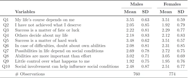
Table 1: Locus of control, youth sample
Males Females
Variables Mean SD Mean SD
Q1 My life’s course depends on me 3.55 0.63 3.51 0.59
Q2 I have not achieved what I deserve 2.05 0.85 1.92 0.79
Q3 Success is a matter of fate or luck 2.22 0.81 2.29 0.77
Q4 Others decide about my life 2.18 0.83 2.12 0.83
Q5 Success is a matter of hard work 3.48 0.62 3.51 0.57
Q6 In case of difficulties, doubt about own abilities 2.08 0.81 2.31 0.85 Q7 Possibilities in life depend on social conditions 2.69 0.78 2.72 0.75
Q8 Abilities are more important than effort 3.02 0.71 3.05 0.69
Q9 Little control over what happens to me 1.92 0.75 1.95 0.76
Q10 Social involvement can help influence social conditions 2.48 0.87 2.51 0.77
# Observations 760 774
In the SOEP youth questionnaire, locus of control is measured by a 10-item question-naire. Each question is answered on a Likert scale ranging from 1 (“disagree completely”) to 4 (“agree completely”). Table 1 gives an overview of the questions and items we use.
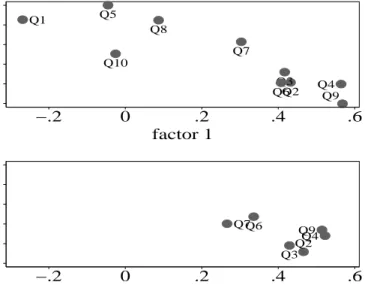
We check whether, given these measurements, locus of control can indeed be represented by a single factor. Conducting a principal component analysis, and calculating the eigen-values of the correlation matrix, we find two eigeneigen-values larger than 1. Hence, the Kaiser criterion (eigenvalue<1) is violated. However, the scree plot analysis displayed in Figure
B.1 reveals an early flattening of the curve, suggesting no more than one or two underlying factors. Furthermore, locus of control is usually conceptualized as referring to a unidimen-sional continuum, ranging from external to internal. Hence, we think that we are making a reasonable decision by extracting a single factor. A scatter plot of the respective factor loadings (FigureB.2), with the first two principal factors on the axis, shows that some items load very highly on the extracted locus of control factor (factor 1), while some other items have a loading close to zero (Q1, Q5, Q8 and Q10). Furthermore, the items with a close to zero loading are items that capture an internal attitude, while the other items mostly capture the external dimension of locus of control. Consequently, we can draw two conclu-sions from this exploratory factor analysis. First, researchers who use an index, constructed for example as the standardized mean of the items, instead of a latent factor, force each of the measurement items to enter the index with an equal weight. Doing this yields a locus of control measure that is flawed by measurement error, and the coefficients are likely to be biased downward due to attenuation bias. Second, in our paper we mostly capture the external attitude dimension of locus of control. For ease of interpretation, in our empirical application we normalize the model such that lower scores of the latent factor are associated with an external locus of control, and higher scores with an internal locus of control. To ensure that our results are not distorted by the inclusion of those items that have a low loading on the locus of control factor, we have conducted robustness checks using only those items loading highly on the first factor. We find that the use of the externalizing items only does not have a major impact on the results.12
12
Results of the robustness check using only the externalizing items can be obtained from the authors upon request.
4.2.3 Covariates
Table2summarizes the covariates used for our analysis, and also shows how the two samples are linked by the schooling equation. To account for family background, socioeconomic sta-tus and labor market conditions, we control for a large range of background variables, as well as for local unemployment rates at the time of education decisions and labor market out-comes, respectively. In addition, Germany has an education system where tracking already takes place after the fourth grade. Hence, to proxy cognitive skills, and to account for the fact that these cognitive skills might affect the items revealing premarket locus of control, we include the primary school teacher track recommendation as a control variable in the measurement system. Because locus of control is estimated from the residual variance net of covariates in the measurement system, covariates included in the measurement equation are a means to purge locus of control of their influence. However, the inclusion of track recom-mendation only proxies cognitive skills and the resulting track type. It cannot account for other conflicting effects such as school quality. Hence, locus of control, as identified in this paper, only captures premarket locus of control, and not necessarily pre-compulsory-school
locus of control. Thus we control for track recommendation, parental education and a large set of other background variables to capture school quality, home investment and cognitive ability. Summary statistics of control variables in the measurement and outcome equations can be found in Tables B.3 and B.4.13
5 Empirical results
The results are presented and discussed in two stages. We first provide a description of the main findings in Section 5.1, with an emphasis on the statistical significance of the impact of locus of control on the different outcomes, and on the fit of our model. Then, we gain
13
Table 2: Samples and included covariates for the measurement system, education, employment and wage equations
Typea Meas. Educ. Empl. Wage
Samples
Youth sample X X (X)b (X)b
Adult sample — X X X
Covariates
Number of siblings D X — — —
% of time in broken family C X X — —
Father dropout B X X X X
Father grammar school B X X X X
Mother dropout B X X — —
Mother grammar school B X X — —
Region: Northc B X X X X
Region: Southc B X X X X
Childhood in large cityd B X X X X
Childhood in medium cityd B X X X X
Childhood in small cityd B X X X X
Track recommendation (highest)e B X — — —
Track recommendation (lowest)e B X — — —
Local unemployment rate C — — X X
Local unemployment rate (edu)f C — X — —
Age of individual C — — X X Cohort 26/30 B — X — X Cohort 31/35 B — X — X Married B — — X X Number of Children C — — X X a
B = Binary, C = Continuous, D = Discrete.
b
Only a small subsample available for these equations.
cBase category isWest Germany. d
Base category isChildhood in countryside.
e
Base category isRecommendation for middle track.
f
more insights in Section 5.2 by conducting some simulations that make it possible to better grasp the magnitude of the impact of locus of control.
5.1 MCMC results
Factor loadings. The factor loadings express how the different measurements and
out-comes are affected by the latent factor. The larger the magnitude of the loadings, the higher the contribution of the corresponding measurements to the distribution of the latent factor. In the education, employment and wage equations, the loadings measure the impact of the factor on the respective outcomes. Cross-model comparisons should however be carefully done: the factor loadings of the different models cannot be directly compared, as their mag-nitude and their sign depend on the normalization retained to set the scale of the factor. We normalize the factor loading of the fourth indicator to −1 in all models, which is a way of anchoring the factor distribution in a real measurement (Cunha and Heckman, 2008).14
However, contrary to Cunha and Heckman (2008), who anchor the factor in earnings, we cannot give an interpretable metric to the latent factor, because of the ordinal nature of the measurement. Moreover, the respective item of the questionnaire used for the normalization might be perceived differently by males and females, and gender comparisons are therefore not straightforward.
Table3summarizes the estimation results for the factor loadings of the different models. The results of the measurement system are in line with our expectations. Typical questions associated with an external locus of control such as ‘Success is a matter of fate or luck’ (Q3) or ‘I have not achieved what I deserve’ (Q2) have negative factor loadings, whereas statements reflecting an internal locus of control, such as ‘My life’s course depends on me’ (Q1), have a positive factor loading. Also, the heterogeneity of these factor loadings is worth noting, as well as the fact that some of them are not significantly different from zero.
14
Table 3: Factor loadings of the model estimated by conditioning labor market outcomes on education [(2) and (4)] and without conditioning on education [(1) and (3)]
Males Females
(1) (2) (3) (4)
Measurement system: Locus of control items
Q1 0.354∗∗∗ (0.087) 0.364∗∗∗ (0.086) 0.423∗∗∗ (0.095) 0.440∗∗∗ (0.101) Q2 -0.735∗∗∗ (0.119) -0.729∗∗∗ (0.116) -0.895∗∗∗ (0.132) -0.938∗∗∗ (0.143) Q3 -0.741∗∗∗ (0.118) -0.743∗∗∗ (0.116) -0.619∗∗∗ (0.107) -0.650∗∗∗ (0.113) Q4 -1.000 — -1.000 — -1.000 — -1.000 — Q5 0.013 (0.074) 0.024 (0.075) 0.026 (0.085) 0.025 (0.089) Q6 -0.640∗∗∗ (0.108) -0.605∗∗∗ (0.102) -0.890∗∗∗ (0.134) -0.916∗∗∗ (0.139) Q7 -0.559∗∗∗ (0.099) -0.565∗∗∗ (0.099) -0.581∗∗∗ (0.105) -0.617∗∗∗ (0.112) Q8 -0.195∗∗∗ (0.072) -0.197∗∗∗ (0.072) -0.107∗ (0.078) -0.112∗ (0.082) Q9 -1.045∗∗∗ (0.175) -1.035∗∗∗ (0.175) -1.781∗∗∗ (0.309) -1.858∗∗∗ (0.332) Q10 -0.122∗∗ (0.067) -0.140∗∗ (0.068) 0.143∗∗ (0.078) 0.146∗∗ (0.080) Education choice S 0.634∗∗∗ (0.134) 0.404∗∗∗ (0.118) 0.444∗∗∗ (0.123) 0.364∗∗∗ (0.127)
Labor market participation
E 0.055 (0.136) -0.021 (0.131) E0 0.757∗∗∗ (0.287) 0.357∗∗ (0.222) E1 -0.126 (0.331) -0.268 (0.286) log Wages Y 0.181∗∗∗ (0.041) 0.121∗∗∗ (0.048) Y0 0.007 (0.060) 0.058 (0.064) Y1 -0.072 (0.086) 0.020 (0.087)
Variance of the latent factor
σ2
θ 0.635∗∗∗ (0.138) 0.622∗∗∗ (0.135) 0.446∗∗∗ (0.092) 0.411∗∗∗ (0.088)
Notes:Factor loading of item 4 (statement reflecting an external locus of control) fixed to -1 to set the scale of the latent factor. Standard errors in brackets. Significance check: */**/*** if zero lies outside the 90%/95%/99% confidence interval of the posterior distribution of the corresponding parameter.
In the outcome system of equations, the factor loading of the education equation is always significant and positive, indicating an actual impact of locus of control. When we do not control for education [columns (1) and (3)], wages appear to be affected by locus of control, whereas this impact vanishes when education is controlled for [columns (2) and (4)]. Hence, with respect to the theoretical framework laid out in Section 3.1, we can conclude that the impact of premarket locus of control on w0t and wt1, denoted by α0 and α1 respectively, is
zero. However, we find that locus of control does have an impact on education decisions (P(S = 1)), and thus on wages in the end. Hence, reverting to Equation (3.1), we can conclude that locus of control does not affect education decisions via higher expected wages (α0,α1), but instead through its impact on the cost of education αC.
So far, no firm conclusions have been made as to the magnitude of the impact of locus of control on education decisions and overall wages. In the following Section5.2, the simulations we conduct make it possible to unravel and quantify the actual impact of locus of control on the different outcomes of interest.
Model fit to actual data. Our model provides a good fit to the data, and especially to
the distribution of wages. Figure 1 displays the observed distribution of wages, along with their posterior predictive distribution for the different specifications. The actual distribution is quite well approximated by the posterior predictive distribution, particularly in the case where the two schooling groups are pooled for the estimation of the wage equation (panels1a
and 1b). When the wage equation is estimated by level of schooling (panels 1c, 1d, 1e and
1f), the fit is somewhat less good. Nevertheless, the Kolmogorov-Smirnov tests we conduct to compare the actual distribution and the posterior predictive distribution never reject the null hypothesis of equal distribution. This result is in great part due to the use of normal mixtures for the error term, allowing for a flexible approximation of the true distribution.
Figure 1: Goodness-of-fit check for wages: posterior predictive (dashed) vs. actual distri-bution (solid) and Kolmogorov-Smirnov test for equal distridistri-butions.
−1 0 1 2 3 4 5 0.0 0.2 0.4 0.6 0.8 1.0 1.2 log wages density KS-test: 0.026 (0.745)
(a) Males, all education levels
−1 0 1 2 3 4 5 0.0 0.2 0.4 0.6 0.8 1.0 1.2 log wages density KS-test: 0.027 (0.799)
(b) Females, all education levels
−1 0 1 2 3 4 5 0.0 0.2 0.4 0.6 0.8 1.0 1.2 log wages density KS-test: 0.042 (0.418)
(c) Males, no higher education
−1 0 1 2 3 4 5 0.0 0.2 0.4 0.6 0.8 1.0 1.2 log wages density KS-test: 0.085 (0.072)
(d) Males, with higher education
−1 0 1 2 3 4 5 0.0 0.2 0.4 0.6 0.8 1.0 1.2 log wages density KS-test: 0.047 (0.479)
(e) Females, no higher education
−1 0 1 2 3 4 5 0.0 0.2 0.4 0.6 0.8 1.0 1.2 log wages density KS-test: 0.055 (0.398)
(f) Females, with higher education
Notes: Model estimated by conditioning labor market outcomes on education (panels1cto1f) and without conditioning on education (panels1aand1b). Kernel density estimation implemented using a Gaussian kernel with bandwidth selected using Silverman’s rule of thumb (Silverman,1986) with the variation proposed byScott(1992). Wages predicted from their posterior distribution using 1,000 replications of the sample. Shaded area represents 95% confidence interval of posterior predictive distribution. Kolmogorov-Smirnov test: Two-sample KS-test with null hypothesis that the actual sample and the posterior predictive sample have the same distribution. p-values in brackets. Exact p-values could not be computed due to ties in the distribution of actual wages.
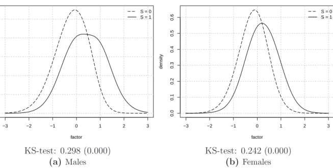
Figure 2: Latent factor distribution by levels of education: people with higher education (S = 1) and without higher education (S = 0).
−3 −2 −1 0 1 2 3 0.0 0.1 0.2 0.3 0.4 0.5 factor density S = 0 S = 1 KS-test: 0.298 (0.000) (a) Males −3 −2 −1 0 1 2 3 0.0 0.1 0.2 0.3 0.4 0.5 0.6 factor density S = 0 S = 1 KS-test: 0.242 (0.000) (b) Females
Notes: Simulation from the estimates of the model using 1,000 replications of the posterior sample. Model estimated without conditioning labor market outcomes on education. Predicted levels of education used (Pr(S= 1) > .5). Kernel density estimation implemented using a Gaussian kernel with bandwidth selected using Silverman’s rule of thumb (Silverman,1986) with the variation proposed byScott(1992). Kolmogorov-Smirnov test: Two-sample KS-test with null hypothesis that the two distributions are the same. p-values in brackets. Exactp-values could not be computed due to ties in the distribution of the latent factor.
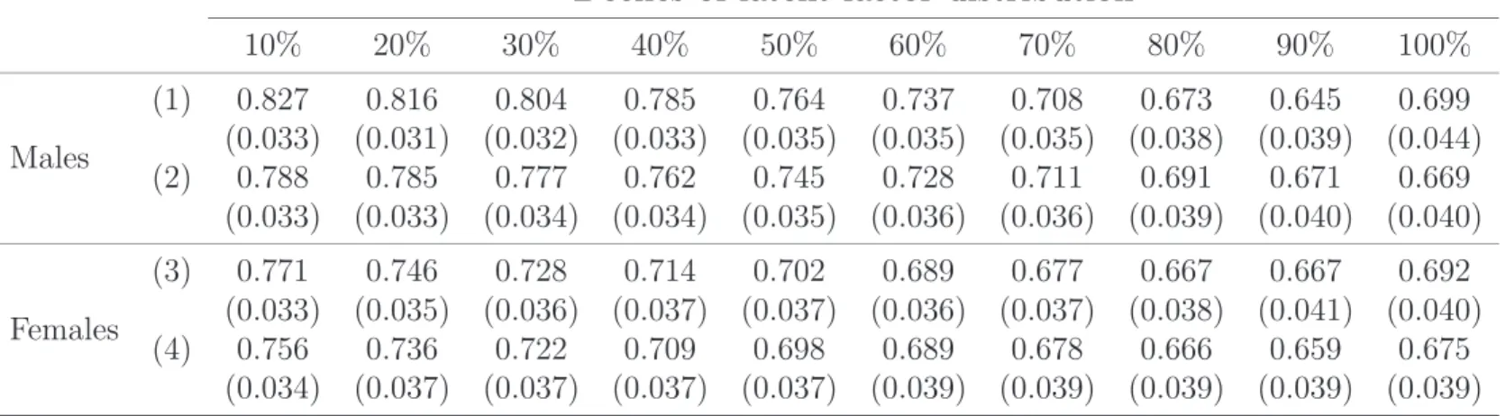
To assess the goodness of fit to the education decision, Table 4 shows the proportion of correct predictions of education achievement for each decile of the latent factor distribution. The fit appears good overall, especially for the lower deciles of the distribution.
5.2 Simulation of the model
To shed more light on the implications of our model, we need to go beyond the mere inter-pretation of the factor loadings. Their statistical significance reveals an impact of locus of control on the outcomes, but is quite uninformative regarding the magnitude of this impact (McCloskey and Ziliak, 1996; Ziliak and McCloskey, 2004). Since the effects of premarket locus of control are intertwined and potentially operate through different channels on wages, the best way to understand our model is to simulate it.
Table 4: Goodness-of-fit check: proportion of correct predictions of education achievement for each decile of the latent factor distribution
Deciles of latent factor distribution
10% 20% 30% 40% 50% 60% 70% 80% 90% 100% Males (1) 0.827 0.816 0.804 0.785 0.764 0.737 0.708 0.673 0.645 0.699 (0.033) (0.031) (0.032) (0.033) (0.035) (0.035) (0.035) (0.038) (0.039) (0.044) (2) 0.788 0.785 0.777 0.762 0.745 0.728 0.711 0.691 0.671 0.669 (0.033) (0.033) (0.034) (0.034) (0.035) (0.036) (0.036) (0.039) (0.040) (0.040) Females (3) 0.771 0.746 0.728 0.714 0.702 0.689 0.677 0.667 0.667 0.692 (0.033) (0.035) (0.036) (0.037) (0.037) (0.036) (0.037) (0.038) (0.041) (0.040) (4) 0.756 0.736 0.722 0.709 0.698 0.689 0.678 0.666 0.659 0.675 (0.034) (0.037) (0.037) (0.037) (0.037) (0.039) (0.039) (0.039) (0.039) (0.039)
Notes: Model estimated by conditioning labor market outcomes on education [(2) and (4)] and without conditioning [(1) and (3)]. Proportions of correct predictions computed for each MCMC replication, corresponding means and standard errors (in brackets) are reported.
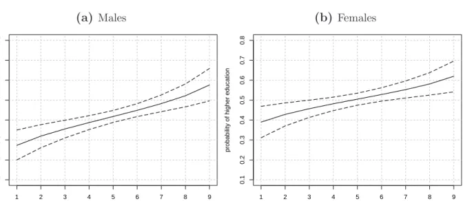
Figure 3: Probability of achieving higher education for each decile of the factor distribution (a) Males 1 2 3 4 5 6 7 8 9 0.1 0.2 0.3 0.4 0.5 0.6 0.7 0.8 deciles
probability of higher education
(b) Females 1 2 3 4 5 6 7 8 9 0.1 0.2 0.3 0.4 0.5 0.6 0.7 0.8 deciles
probability of higher education
Notes: Simulation from the estimates of the model using 10,000 replications of the posterior sample. Model estimated conditioning labor market outcomes on education. 95% confidence band between dashed lines.
Figure 2 plots the estimated posterior distribution of the latent factor by levels of ed-ucation, and shows that people who achieve higher education have a more internal locus of control. For males, the gap between the two schooling groups is even wider, revealing some gender differences in the way locus of control influences education decisions. The Kolmogorov-Smirnov test confirms that the discrepancy between the two distributions is statistically significant for both genders.
To get more insight on the impact of premarket locus of control on later outcomes, we can investigate how the wage of a given individual would be affected if she were exogenously moved along the distribution of the latent factor, for a given set of observed characteristics
XY (Heckman et al., 2006b). For this purpose, we compute the expected wage for different quantiles of the distribution of the factor, conditional on a given set of covariates XY. The Gibbs algorithm we implement to estimate our model generates a sample of the model parameters from their conditional distribution that can be used as follows to approximate
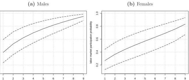
Figure 4: Probability of labor market participation for people without higher education for each decile of the factor distribution
(a) Males 1 2 3 4 5 6 7 8 9 0.2 0.4 0.6 0.8 1.0 deciles labor mar k et par ticipation probability (b) Females 1 2 3 4 5 6 7 8 9 0.2 0.4 0.6 0.8 1.0 deciles labor mar k et par ticipation probability
Notes: Simulation from the estimates of the model using 10,000 replications of the posterior sample. Model estimated
conditioning labor market outcomes on education. 95% confidence band between dashed lines.
the expected wage for each quantile qθ of the factor distribution: 1 M M X m=1 XYβY(m)+qθ(m)α(Ym),
for a set of M simulated parameters (βY(1), αY(1)), . . . ,(βY(M), α(YM)). The quantile of the la-tent factor qθ(m) also has a superscript (m), since it depends on the variance of the factor
σθ2(m), and therefore varies during the MCMC sampling. Similarly, the schooling and labor market participation probabilities in the qth quantile of the latent factor distribution can be
approximated by: 1 M M X m=1 ΦXSβ (m) S +q (m) θ α (m) S , 1 M M X m=1 ΦXEβ (m) E +q (m) θ α (m) E ,
respectively, where Φ(·) denotes the cdf of the standard normal distribution. More
specifi-cally, the simulations we present rely on the deciles of the distribution. In the following, our simulations are performed for the mean individual of the corresponding sample.
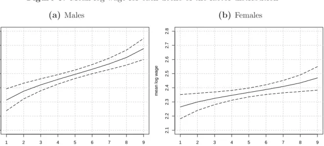
Figure 5: Mean log wage for each decile of the factor distribution (a) Males 1 2 3 4 5 6 7 8 9 2.1 2.2 2.3 2.4 2.5 2.6 2.7 2.8 deciles mean log w age (b) Females 1 2 3 4 5 6 7 8 9 2.1 2.2 2.3 2.4 2.5 2.6 2.7 2.8 deciles mean log w age
Notes:Simulation from the estimates of the model using 10,000 replications of the posterior sample. Model estimated without conditioning labor market outcomes on education. 95% confidence band between dashed lines.
From Figure 3, locus of control appears to have a large impact on the schooling decision, since moving the mean individual from the first to the last decile of the distribution results in a 0.30 point increase in the probability of achieving higher education for males, and a 0.23 point increase for females. Similarly, Figure4shows that in the group of people who did not achieve higher education, locus of control has a huge impact on labor market participation. This effect is more or less linear for females, whereas for males the concavity of the curve indicates that people in the low deciles are more affected than people in the higher deciles of the distribution. Concerning wages, Figure 5 shows that if the mean individual could be moved exogenously from the first to the 9th decile of the locus of control distribution, this
would corresponds to an increase in hourly wages of roughly 4.40 Euros for the mean male individual, and of roughly 2.20 Euros for the mean female individual.
At first sight, the effect of locus of control on education choice and labor market outcomes seems large. For instance, the mean male individual would earn 36% more in the last decile than in the first one. However, it is unrealistic to see an individual move all the way across the distribution. People are more likely to make small moves from one decile to the adjacent
ones, and Figures 3 to 5 show that in the middle of the distribution, the locus of control effect is much smaller.
5.3 Some remarks on the results
In summary, we find an effect of locus of control on schooling probabilities, where males are more affected than females. Moving the mean individual in the distribution of the latent factor substantially changes her/his wage. However, this overall effect only operates through the channel of schooling. This finding that premarket locus of control influences schooling is in line withColeman and DeLeire(2003), although in their paper the mechanism through which locus of control affects schooling is different, as it only works through wage expectations.
Our results seem somewhat contrary to the more direct link between locus of control and wages that been found in some of the literature (Heckman et al.,2006b;Heineck and Anger,
2010). Three different answers can be put forward to address this apparent contradiction. First, the term ‘noncognitive skills’ is very often used as a generic expression encompassing a lot of different personal abilities and traits, sometimes leading to confusion. A compar-ison of results is possible only if the same concept is used. For instance, Heckman et al.
(2006b) find a significant effect of noncognitive skills on wages. However, they use a single underlying factor for noncognitive skills constructed from two psychometric tests, namely the Rosenberg self-esteem scale and the Rotter scale. This composite factor thus captures a different dimension than our factor, especially since it loads more on the self-esteem scale than on the locus of control scale in their empirical study. Second, and more importantly, we focus on premarket locus of control as a measure of locus of control that is independent of labor market experience. As a consequence, our findings differ from the results presented by Heineck and Anger (2010) who find a strong and significant impact of locus of control on wages, even after controlling for education. One reason could be that the authors do not
estimate separate models by education level. More likely, however, the difference in results arises because of the use of contemporaneous measurements in their study, while we focus on the impact ofpremarket locus of control. Third, we only look at a sample of young labor market entrants. At this stage, wage setting is likely to be merely a function of formal qual-ifications. Hence, only after individuals have entered the labor market, a complex dynamic interaction process begins. While working on-the-job, individuals learn about their abilities, while at the same time employers adapt their knowledge about an individual’s locus of con-trol. As a result, a positive interdependence between locus of control and wages may arise (such as the one found by Heineck and Anger, 2010). Additional analyses not displayed in this paper show that the correlation between locus of control and wages does indeed increase with age and experience of the agents. Whether this is the result of reverse causality or learning of employers is an interesting topic left for future research. One explanation may be that although early locus of control does not influence wages directly, it may influence late locus of control which in turn is directly rewarded on the labor market. We leave it for future research to find out whether there exists a constant and invariable component to personality traits in general, and to locus of control in particular. Such a component may be extracted using dynamic factor models, and would require repeated measurements of locus of control over large parts of the life-cycle.
6 Conclusion
In this paper, we use Bayesian factor structure models to investigate how locus of control influences education decisions and wages. Using advanced econometric methods, we show that such recent methods can serve as a solution measurement error and endogeneity prob-lems, especially if researchers are confronted with truncated life cycle data, as is very often the case for research at the intersection of psychology and economics.
We establish that an individual’spremarket locus of control substantially raises the prob-ability of choosing higher education. We also show that locus of control influences wages through schooling, but that there is no direct impact on wages once schooling is controlled for. Thus, in a framework where schooling decisions depend on relative lifetime earnings returns for each schooling level, net of the costs of obtaining either level of education, we can infer from our results that premarket locus of control, as measured at the age of 17, is not directly rewarded as a skill on the labor market. Instead, it is a personality trait that influences the non-pecuniary costs of education.
Our work conveys important policy implications. If some personality traits, such as locus of control, influence the cost of education but not outcomes directly, these individual characteristics may keep individuals from studying who, once they reach the labor market, are no less successful than other individuals. If these individuals are at high risk of dropping out of school, early personality tests and targeted mentoring of students with an external locus of control are a means to countervail skill shortages in society.
References
Andrisani, P. J. (1977): “Internal-External Attitudes, Personal Initiative, and the Labor Market Experience of Black and White Men,”Journal of Human Resources, 12, 308–328. ——— (1981): “Internal-External Attitudes, Sense of Efficacy, and Labor Market
Experi-ence: A Reply to Duncan and Morgan,” Journal of Human Resources, 16, 658–66. Becker, G. S.(1964): Human Capital: A Theoretical and Empirical Analysis, With Special
Reference to Education, New York: National Bureau of Economic Research.
Borghans, L., A. L. Duckworth, J. J. Heckman, and B. ter Weel (2008): “The
Economics and Psychology of Personality Traits,”Journal of Human Resources, 43, 972– 1059.
Bowles, S. and H. Gintis (1976): Schooling in Capitalist America: Educational Reform and the Contradictions of Economic Life, Routledge.
——— (2002): “Schooling in Capitalist America Revisited,” Sociology of Education, 75, 1–18.
Bowles, S., H. Gintis, and M. A. Osborne (2001): “The Determinants of Earnings: A Behavioral Approach,” Journal of Economic Literature, 39, 1137–1176.
Caliendo, M., D. A. Cobb-Clark, and A. Uhlendorff (2010): “Locus of Control
and Job Search Strategies,” Institute for the Study of Labor (IZA) Discussion Paper No. 4750.
Card, D.(1999): “The causal effect of education on earnings,”Handbook of labor economics, 3, 1801–1863.
Carneiro, P., K. Hansen, and J. J. Heckman (2003): “Estimating Distributions of Treatment Effects with an Application to the Returns to Schooling and Measurement of the Effects of Uncertainty on College Choice,” International Economic Review, 44, 361–422.
Cebi, M.(2007): “Locus of Control and Human Capital Investment Revisited,” Journal of Human Resources, 42, 919–932.
Coleman, J. S. (1968): “Equality of Educational Opportunity,” Equity & Excellence in Education, 6, 19–28.
Coleman, M. and T. DeLeire (2003): “An Economic Model of Locus of Control and the Human Capital Investment Decision,” Journal of Human Resources, 38, 701–721.
Cowles, M. K. (1996): “Accelerating Monte Carlo Markov Chain Convergence for
Cumulative-Link Generalized Linear Models,” Statistics and Computing, 6, 101–111. Cunha, F. and J. J. Heckman (2008): “Formulating, Identifying and Estimating the
Technology of Cognitive and Noncognitive Skill Formation,” Journal of Human Re-sources, 43, 738–782.

![Table 3: Factor loadings of the model estimated by conditioning labor market outcomes on education [(2) and (4)] and without conditioning on education [(1) and (3)]](https://thumb-us.123doks.com/thumbv2/123dok_us/491677.2558218/27.1263.261.932.204.724/factor-loadings-estimated-conditioning-outcomes-education-conditioning-education.webp)