2018
Random forest robustness, variable importance,
and tree aggregation
Andrew Sage
Iowa State UniversityFollow this and additional works at:https://lib.dr.iastate.edu/etd
Part of theStatistics and Probability Commons
This Dissertation is brought to you for free and open access by the Iowa State University Capstones, Theses and Dissertations at Iowa State University Digital Repository. It has been accepted for inclusion in Graduate Theses and Dissertations by an authorized administrator of Iowa State University Digital Repository. For more information, please [email protected].
Recommended Citation
Sage, Andrew, "Random forest robustness, variable importance, and tree aggregation" (2018).Graduate Theses and Dissertations. 16453.
by
Andrew John Sage
A dissertation submitted to the graduate faculty in partial fulfillment of the requirements for the degree of
DOCTOR OF PHILOSOPHY
Major: Statistics
Program of Study Committee: Ulrike Genschel, Co-major Professor
Dan Nettleton, Co-major Professor Daniel Nordman
Craig Ogilvie Vivekananda Roy
The student author, whose presentation of the scholarship herein was approved by the program of study committee, is solely responsible for the content of this dissertation. The
Graduate College will ensure this dissertation is globally accessible and will not permit alterations after a degree is conferred.
Iowa State University Ames, Iowa
2018
DEDICATION
To my family and friends who encourage me with their words and inspire me with their example.
TABLE OF CONTENTS
Page
ACKNOWLEDGEMENTS . . . vi
ABSTRACT . . . vii
CHAPTER 1. GENERAL INTRODUCTION . . . 1
1.1 Background . . . 1
1.2 Overview . . . 2
1.2.1 Partitioning and Tree Aggregation . . . 2
1.2.2 Variable Importance . . . 3
1.2.3 Robustness . . . 3
1.3 Role of Authors . . . 4
CHAPTER 2. TREE AGGREGATION FOR RANDOM FOREST CLASS PROBA-BILITY ESTIMATION . . . 5
2.1 Introduction . . . 6
2.2 Random Forest Fundamentals . . . 8
2.2.1 Partitioning . . . 8 2.2.2 Tree Aggregation . . . 10 2.2.3 Tuning Parameters . . . 15 2.3 Simulation Study . . . 16 2.4 Data Applications . . . 25 2.5 Conclusions . . . 33
CHAPTER 3. RANDOM FOREST VARIABLE IMPORTANCE IN THE
PRES-ENCE OF MISSING DATA . . . 37
3.1 Introduction . . . 38
3.2 Variable Importance and Missing Values . . . 41
3.2.1 Permutation Importance . . . 41
3.2.2 Imputation of Missing Values . . . 42
3.3 Simulation Study . . . 47
3.3.1 Design . . . 47
3.4 Data Applications . . . 53
3.5 Conclusions . . . 58
CHAPTER 4. A ROBUST RESIDUAL-BASED APPROACH TO RANDOM FOR-EST REGRESSION . . . 63
4.1 Introduction . . . 64
4.2 Background . . . 67
4.2.1 Random Forest Background . . . 67
4.2.2 Prior Robust Aggregation Approaches . . . 67
4.2.3 Prior Robust Splitting . . . 71
4.3 RF-LOWESS Method . . . 71
4.3.1 Motivation and Algorithm . . . 71
4.3.2 Illustrative Example . . . 75
4.3.3 Parameter Tuning . . . 80
4.4 Simulations & Real Data Results . . . 82
4.4.1 Simulation Study . . . 82
4.4.2 Impact of Weighted Cross-Validation . . . 91
4.5 Conclusions . . . 98
4.6 APPENDIX: Additional Details and Results . . . 102
4.6.1 Li & Martin’s Huber Forest Algorithm . . . 102
4.6.2 Additional Simulation Results . . . 103
CHAPTER 5. GENERAL CONCLUSION . . . 107
ACKNOWLEDGEMENTS
I would like to acknowledge several members of the Iowa State University faculty who have been influential in my studies and research. I am especially grateful to my Co-major Professors Ulrike Genschel and Dan Nettleton for their valuable advice, which extends far beyond the writing of this dissertation. I would like to thank Professors Cinzia Cervato and Craig Ogilvie for giving me the opportunity to apply my research in an important and meaningful context. I am grateful to Professors Ogilvie, Daniel Nordman, and Vivekananda Roy for serving on my committee and to Professors Nordman and Roy, whose courses in-creased my understanding and appreciation of statistical theory. I would also like to thank Professor Stephen Vardeman, whose course in statistical machine learning greatly enhanced my understanding of the topics at the heart of this dissertation.
I am also grateful to those who were influential in my learning prior to my studies at Iowa State. Professor Stephen Wright of Miami University first introduced me to the excitement of performing original research. Professors Jim Hartman, Pam Pierce, and John Ramsay of The College of Wooster helped inspire my interest in learning mathematics and statistics as an undergraduate.
Finally, I would like to acknowledge the students I have had the pleasure of teaching at Iowa State University, Miami University, and Bloomfield High School. Working with them has provided me with energy that fuels my research.
ABSTRACT
Random forest methodology is a nonparametric, machine learning approach capable of strong performance in regression and classification problems involving complex datasets. In addition to making predictions, random forests can be used to assess the relative importance of explanatory variables. In this dissertation, we explore three topics related to random forests: tree aggregation, variable importance, and robustness. In Chapter 2, we show that the method of tree aggregation used in one popular random forest implementation can lead to biased class probability estimates and that it is often beneficial to combine the tree partitioning algorithm used in one implementation with the aggregation scheme used in another. In Chapter 3, we show that imputing missing values proir to assessing variable importance often leads to inaccurate variable importance measures. Using simulation studies, we investigate the impact on variable importance of six random-forest-based imputation techniques and find that some techniques are prone to overestimating the importance of variables whose values have been imputed, while other techniques tend to underestimate the importance of such variables. In Chapter 4, we propose a new robust approach for random forest regression. Adapted from a popular approach used in polynomial regression, our method uses residual analysis to modify the weights associated with training cases in random forest predictions, so that outlying training cases have less impact. We show, using simulation studies, that this approach outperforms existing robust techniques on noisy, contaminated datasets.
CHAPTER 1.
GENERAL INTRODUCTION
1.1
Background
Since its creation by Breiman (2001), random forest methodology has emerged as a pow-erful nonparametric, machine learning approach for regression and classification. Based on ensembles of decision trees, random forests routinely handle nonlinear relationships and inter-actions, making them a popular choice for predictions involving complex datasets. Random forests are implemented in severalR (R Core Team, 2016) packages includingrandomForest
(Liaw and Wiener, 2002), randomForestSRC (Ishwaran et al., 2008; Ishwaran and Kogalur, 2007, 2016), and party (Hothorn et al., 2006a; Strobl et al., 2007, 2008).
Random forests consist of many individual classification or regression trees (Breiman et al., 1984), which are grown by recursively performing binary splits on training data. Individual decision trees are low bias, high variance predictors. Averaging predictions across a large number of trees, as is done in a random forest, reduces the variance of the resulting predictor, while maintaining low bias. In order to ensure that trees differ substantially enough to achieve this variance reduction, randomness is introduced in the tree-growing process in the following two ways:
1. Each tree is grown from a different bootstrap sample of the training data.
2. For each split, a randomly selected subset of explanatory variables is considered, rather than considering all explanatory variables.
Let{(x1, y1),(x2, y2), . . . ,(xn, yn)}, represent a set of training data, which are the result
distribution. In a regression setting, a random forest provides an estimate of the conditional mean, E(Y|x). In a classification problem, a random forest can be used to predict the most likely response category, or to estimate P(Y =c|x) =E[1(Y =c)|x], the conditional probability thatY takes on response categoryc. Note that1(·) represents a generic indicator function.
Meinshausen (2006) showed that a random forest prediction for a new case can be ex-pressed as a weighted average of y1, y2, . . . yn. This insight provides a method for estimating
quantiles of the conditional distribution of Y givenx. Such estimates can be obtained using the quanregForest package (Meinshausen, 2016) inR.
1.2
Overview
1.2.1 Partitioning and Tree Aggregation
Several techniques have been proposed for determining splits in training data when grow-ing decision trees. The randomForestand randomForestSRC packages implement the Clas-sification and Regression Tree (CART) algorithm (Breiman et al., 1984). Although widely popular, this approach has been shown to favor splits based on explanatory variables that take on many different values, and potentially fails to take advantage of information provided by categorical predictors (Hothorn et al., 2004, 2006a,b). The party package implements conditional inference trees (Hothorn et al., 2006b), in which splits are determined using per-mutation tests. In addition to the differences in partitioning, tree predictions are aggregated differently in party than in randomForest. In Chapter 2, we show that the aggregation scheme used by party can result in biased class probability estimates in classification prob-lems. Using two real datasets, in which probability estimates are of interest, we show that combining the partitioning approach used in party with the aggregation technique imple-mented inrandomForest yields results that outperform either technique individually.
1.2.2 Variable Importance
One popular feature of random forests is their ability to quantify the importance of explanatory variables in prediction. Roughly speaking, the importance of an explanatory variable Xj is estimated by considering the decrease in predictive accuracy when values of
Xj are randomly permuted, thereby removing any association between Xj and Y. A more
thorough description of this process is given in Chapter 3.
Measuring variable importance becomes increasingly complicated when data are missing. Hapfelmeier et al. (2012, 2014a,b) introduce an approach for estimating variable importance in such settings. This approach is intended to capture the value of the information provided by the data present, and variables with large amounts of missing data are often ranked as less important than they would be if complete data were available. While this is not unreasonable, there are many applications in which a practitioner might wish to estimate how important a predictor variable would be if complete data were available. In these situations, missing values are often imputed before variable importance is estimated via random forests. In Chapter 3, we consider six popular random forest imputation techniques and show that some of these are prone to underestimating, or perhaps more surprisingly, overestimating the importance of variables whose missing values have been imputed. Our study provides insight on which imputation approaches are most appropriate when the primary objective is to measure the importance of explanatory variables.
1.2.3 Robustness
Because random forest predictions are highly local, they are not as susceptible to the in-fluence of outliers as other techniques such as linear regression. However, Roy and Larocque (2012) showed that improvements in performance can be achieved when robust measures are implemented in random forest regression. The estimated 0.5 quantile of the conditional
distribution for Y given X is a robust predictor (Meinshausen, 2006; Roy and Larocque, 2012). Li and Martin (2017) showed that modifying the training case weights described by Meinshausen potentially improves robustness. We further explore this idea, introducing a new robust approach for iteratively adjusting training case weights in Chapter4 of this dis-sertation. Our approach is motivated by the robust approach for locally weighted polynomial regression introduced by Cleveland (1979). We use residual analysis to identify and down weight training cases with outlying response values, and show through simulations that this approach achieves strong performance on noisy, contaminated training data.
1.3
Role of Authors
Andrew Sage performed the investigations and was the primary author for all papers included in this dissertation. Ulrike Genschel and Dan Nettleton provided advice on the direction of the research and contributed to editing each of the manuscripts.
CHAPTER 2.
TREE AGGREGATION FOR RANDOM
FOREST CLASS PROBABILITY ESTIMATION
A paper submitted to Statistical Analysis and Data Mining Andrew J. Sage, Ulrike Genschel, and Dan Nettleton
Abstract
In classification problems, random forests are often used to estimate the probability of a new case falling into each of C possible categories. These probabilities are routinely of interest, for example, in risk analysis. Different methods have been proposed for both growing random forests and aggregating predictions from individual trees, but comparative studies are limited. In this paper, we compare and contrast prominent random forest tech-niques, with particular emphasis on the aggregation of tree predictions. We consider two real datasets where class probability estimates are of interest, and demonstrate that com-bining the partitioning algorithm used in one approach with the aggregation technique used in another can result in performance that is superior to either approach individually.
2.1
Introduction
Random forest methodology is a well-known approach for classification and regression problems that is especially useful when there are a large number of predictor variables, or when many possible interactions exist. Introduced by Breiman (2001), random forests can be used to estimate the probability of an unobserved categorical response variable Y taking on category c forc= 1,2, . . . , C.
Two of the most popular approaches for growing random forests are implemented using the randomForest(Liaw and Wiener, 2002) andparty (Hothorn et al., 2006a; Strobl et al., 2007, 2008) packages inR(R Core Team, 2016). TherandomForestpackage grows individual trees using Breiman’s Classification and Regression Tree (CART) algorithm (Breiman et al., 1984). ThecForestfunction in theparty package grows random forests using permutation tests to determine splits. Hothorn et al. (2006b) refer to trees grown in this manner as conditional inference trees.
Hothorn et al. (2006b) and Strobl et al. (2007) show that CART leads to biased vari-able selection, favoring continuous predictors or categorical predictors with many possible categories. Strobl et al. (2007) show that unbiased measures of variable importance can be obtained with cForest, when trees are grown from subsamples, rather than bootstrap samples, of the training data. Conditional inference trees have been employed extensively in the applied literature, especially when measuring variable importance (c.f. Scott et al. (2011); Arpaci et al. (2014)). While it stands to reason thatcForestshould benefit from its ability to utilize information contained in predictor variables that take on only a few values, its predictive performance relative to randomForest, under specific loss functions, has not been extensively studied.
The randomForest and party packages differ not only with respect to partitioning, but also in the way that information from individual trees is aggregated to obtain probability
estimates. A description of thecForestapproach can be found in Hothorn et al. (2004) while Meinshausen (2006) discusses the algorithm used by randomForest. These papers focus primarily on regression and survival analysis. Less attention has been given in the literature to the effect of aggregation schemes on probability estimates in classification problems.
In this work, we examine probability estimates resulting from the aggregation schemes implemented by randomForest and cForest in classification problems. We show that the different aggregation approaches sometimes result in considerable discrepancies between the probability estimates, even if applied to the exact same forest. While thecForest partition-ing approach is capable of superior performance in applications with a mix of categorical and numerical predictors, it is prone to overestimating the probability of the most likely re-sponse, while underestimating the probability of less likely outcomes. This bias results from a disproportionate influence of large, pure terminal nodes. Systematically underestimating the probability of unlikely events can result in serious consqeuences when the probability estimates are used, for example, to assess the risk of risk of defect or failure of large invest-ments.
We further show that overestimation of the probability of the most likely outcome is most severe when tuning parameters are set to allow for deep trees with small terminal nodes. Requiring terminal nodes much larger than cForest defaults helps mitigate this concern, but does not eliminate it entirely. We demonstrate that combining the cForestpartitioning algorithm with the aggregation approach used by randomForest can lead to performance superior to either technique individually. Finally, we show that optimal settings for tuning parameters pertaining to terminal nodesize depend heavily on the aggregation approach used and that the randomForest aggregation approach is less sensitive to the choice of tuning parameters than the cForestapproach.
We structure the remainder of the manuscript as follows. In Section 2.2, we provide an overview of the partitioning algorithms employed by randomForest and by cForest. We
continue with a detailed discussion of the aggregation approaches utilized by each package, and conclude the section with a discussion of random forest tuning parameters. In Section
2.3, we conduct a simulation study and demonstrate that the cForest aggregation scheme can lead to biased probability estimates. In Section 2.4, we assess the performance of the
randomForest and cForest partitioning and aggregation approaches on two real datasets, where class probabilities are of interest. We summarize our conclusions in Section 4.5.
2.2
Random Forest Fundamentals
Although we focus primarily on tree aggregation in this study, we begin with a brief overview of the partitioning algorithms under consideration to grow a random forest on a set of training data, consisting of n observations on ppredictor variables.
2.2.1 Partitioning
The CART algorithm, implemented in randomForest, grows each individual tree using a newly generated bootstrap sample of the training set. Let 1(·) denote a generic indicator function that takes value one if the condition specified within parentheses is true and zero otherwise. A node is split, i.e. partitioned into two resulting subnodes, based on the values of a function of the form 1(x ∈ S), where x is one of the predictor variables and S is a set of the form (−∞, τ], τ ∈ R, if x is quantitative or a subset of categories if x is categorical. The variable x and the set S are selected so that the two resulting subnodes achieve maximal homogeneity with respect to the response variable. Although homogeneity of the response values in a node can be measured in multiple ways, the most common approach for a categorical response variable involves the use of the Gini index as a measure
of impurity. The Gini index for a node P is defined as IP =nP · C X c=1 πP(c)[1−πP(c)], (2.1)
wherenP denotes the number of training cases in nodeP, andπP(c) represents the proportion
of cases in P with response c, c= 1,2, . . . , C. If all training cases in node P have the same response, IP = 0, while the value of IP increases as the node becomes less pure. Let L and
R denote the nodes resulting from a possible split. Then the decrease of impurity (increase in homogeneity) associated with the split can be measured by
∆I(P, L, R) =IP −(IL+IR). (2.2)
For each split in a tree, a new subset of m < p predictor variables is randomly selected. Considering each variable in the randomly selected subset, all possible splits are evaluated, and the split that maximizes ∆I(P, L, R) is selected. Partitioning continues until all nodes are either pure, or smaller than a predetermined size, or until all training cases have identical values for the predictor variables randomly selected for the split.
When a set of predictor variables contains both continuous and categorical variables, the CART algorithm has been shown to favor splits on continuous predictors or categorical predictors with many possible categories. Because relatively many splits are possible for such variables, high values of ∆I(P, L, R) can often be achieved even for a variable not strongly associated with the response. As a consequence, CART-based partitioning sometimes fails to effectively utilize information provided by predictor variables with only a few possible splits. This issue is illustrated by Hothorn et al. (2006b) and Strobl et al. (2007).
Hothorn et al. (2006b) address the variable selection bias shown by CART using permu-tation tests, rather than Gini index, to determine the best split for each node. Specifically, within each node, upon randomly selecting a subset of predictor variables, permutation tests are used to first identify the predictor variable having the strongest association with the re-sponse variable and then to determine the best split on that variable. Because the choice of
which variable to split on is based on performing a single permutation test for each variable, regardless of the number of possible splits on that variable, this method does not suffer from the selection bias that affects CART-based partitioning. Strobl et al. (2007) show that while conditional inference trees reduce variable selection bias, compared to CART, this bias is not removed entirely unless trees are grown from subsamples, rather than bootstrap samples. This modification is implemented as the default setting for the cForest function.
Regardless of the method used to grow trees, once trees have been grown, predictions are made by moving a new case through each tree in accordance with its predictor variable values and the splitting rules determined from the training data. Once a case lands in a terminal node, response categories of training cases in that terminal node are used to estimate the probability of the new case taking on each possible response category. There are, however, multiple ways that this information is combined across trees to estimate each probability. These aggregation techniques are discussed in Subsection2.2.2.
2.2.2 Tree Aggregation
In the following, we describe three different aggregation approaches used by therandomForest
and cForest algorithms. We begin by introducing notation applicable to all three aggrega-tion approaches.
Let {(x1, y1),(x2, y2), . . . ,(xn, yn)} denote a set of training data of size n, where yi ∈ {1,2, . . . , C} for i = 1, . . . , n; that is yi falls into one of C possible response categories.
Given a new case (x∗, Y∗), where Y∗ is unknown, we seek to estimate P(Y∗ = c), the probabilityY∗ takes the value associated with response category cfor c∈ {1,2, . . . , C}. For
each aggregation scheme, an estimate of P(Y∗ =c) is given by b P(Y∗ =c|x∗) = T X t=1 wt(x∗)ht(x∗, c) T X t=1 wt(x∗) , (2.3)
for some functions wt and ht, where wt represents the weight given to tree t and ht
rep-resents a prediction or probability estimate associated with tree t. Choices for wt and ht
differ by aggregation scheme and will be discussed in more detain in sections2.2.2.1–2.2.2.3. Expressions forwt and ht depend on additional quantities that are defined as follows.
Let bt(j) denote the number of times training case j occurs in the bootstrap sample or
subsample used to grow treetfort= 1,2, . . . , T. For each treet and new casex∗, letNt(x∗)
denote the collection of indices of training cases lying in the same terminal node asx∗. That is,
Nt(x∗) = {j : (xj, yj) is in the same terminal node as x∗ for tree t, j = 1,2, . . . n}.
Let
at(x∗, c) = X
j∈Nt(x∗)
bt(xj)1(yj =c), (2.4)
denote the number of categoryc responses in the terminal node containingx∗ in tree t.
2.2.2.1 Equal Weighting of Tree Proportions (EW)
Since each tree produces an estimate of P(Y∗ =c|x∗), which is given by the proportion of training cases in the same terminal node as x∗ that have response category c, an overall random forest estimate can be found by averaging these proportions across trees. All trees
are given equal weight so wt(x∗) = 1, resulting in the estimate b PEW(Y∗ =c|x∗) = T X t=1 ht(x∗, c) T , (2.5)
where ht(x∗, c) represents the proportion of training cases in the same terminal node as x∗
that take on responsec, in tree t, i.e.,
ht(x∗, c) = at(x∗, c) X j∈Nt(x∗) bt(xj) . (2.6)
For a binary response variable, Y, this aggregation approach can be implemented using the randomForest package by treating Y as a numeric variable, taking on values 0 and 1. When the response variable is numeric, i.e., in regression, randomForest predicts the value of a response variableY∗, by averaging the response values for all training cases in the same terminal node as x∗ followed by averaging these predictions across all trees. Estimating the expected response, E (1(Y∗ =c|x∗)), in this manner results in the estimatePbEW(Y∗ =c|x∗)
given in (2.5).
We note that in regression problems, randomForest determines the best split using a mean square error loss function, instead of the Gini index, which is used for classification. However, mean square error and Gini index are equivalent for binary response variables. Therefore, this approach can be implemented directly, using random forest regression when C = 2. For C > 2, one can grow a random forest using Gini index, and then calculate probability estimates in accordance with (2.5) and (2.6).
2.2.2.2 Proportional Weighting of Tree Proportions (PW)
ThecForestaggregation approach assigns weights to individual training cases according to the number of times a training case lands in the same terminal node asx∗. This approach
is equivalent to averaging proportions given by individual trees, except the weight of tree t is proportional to the number of training cases in the same terminal node as x∗ in tree t.
Let ht(x∗, c) be defined as in (2.6). Then
wt(x∗) = X
j∈Nt(x∗)
bt(xj). (2.7)
An estimate of P(Y∗ =c|x∗) is given by
b PP W(Y∗ =c|x∗) = T X t=1 wt(x∗)ht(x∗, c) T X t=1 wt(x∗) . (2.8)
The probability estimate in (2.8) can be equivalently obtained by pooling, across all trees in a forest, the contents of the terminal nodes containingx∗ and then finding the proportion of all response values in the pool equal to c.
2.2.2.3 Tree Voting (TV)
For completeness, we include a description of a third possible aggregation approach that is implemented in the randomForest package when the response variable is categorical.
In this approach, each tree predicts the response category for a new case by taking the most frequently occurring response in the terminal node containing x∗. That is, each tree casts a “vote” for the response category it determines to be most probable. The function ht(x∗, c) in (2.3), can be written as
ht(x∗, c) =1(at(x∗, c)> at(x∗, c0) for all c0 6=c). (2.9)
In the case of a tie, i.e., if max{(at(x∗, c) : c = 1, . . . , C} is achieved for more than once
choice of c, let ˜c represent the class that is randomly chosen from the maximizers and set ht(x∗,˜c) = 1, and ht(x∗,˜c) = 0 for all c6= ˜c.
The probability that a new case takes on response category c is estimated by the pro-portion of trees voting for categoryc. Predictions from each tree are given equal weight, so wt(x∗) = 1 fort= 1. . . T and for all x∗. Therefore, equation (2.3) results in the probability
estimate b PT V(Y∗ =c|x∗) = T X t=1 ht(x∗, c) T , (2.10) where ht(x∗, c) is as defined in (2.9).
While this technique is popular when the task is simply classification (i.e. determining the most likely response category), it is ill-suited for class probability estimation. This method only considers the most likely response from each tree, without accounting for the proportion of cases taking on a particular response category. These proportions contain valuable information when class probability estimates are of interest. For the remainder of the paper, we therefore focus on the aggregation approaches described in sections2.2.2.1and
2.2.2.2.
2.2.2.4 Proposed Method
It is important to note that any aggregation approach can be used with any parti-tioning algorithm. While cForest implements proportional weighting of tree proportions, this choice is independent of the cForest partitioning algorithm. We propose combining the cForest partitioning approach, which implements conditional inference trees, with the equally weighted tree aggregation approach used by randomForestfor regression. We show, in the ensuing sections, that this combined approach can be advantageous. Code for obtain-ing estimates in this manner is available on Github (Sage, 2017).
Before we study and compare performance of the partitioning and aggregation algorithms discussed in this section, we briefly explain the role of tuning parameters, necessary for the
implementation of randomForest and cForestin R. These tuning parameters must be set carefully in order to achieve each method’s optimal performance.
2.2.3 Tuning Parameters
An important consideration in the use of random forest methodology is the choice of tuning parameters. In randomForest, there are two parameters that must be set with care. The first is the number of explanatory variables to consider for each split. The second is a terminal nodesize parameter, which is defined so that nodes smaller than this value are not split any further. These parameters are called mtry and nodesize, respectively. In
cForest, there are three related tuning parameters. Themtry parameter is defined the same way in cForest as in randomForest, and the minsplit parameter in cForest is analagous to nodesize. In addition, cForest uses a parameter called minbucket which specifies the smallest nodesize allowed for a terminal node. For the remainder of the paper, we refer to the nodesize, minsplit, and minbucket collectively asterminal nodesize parameters.
Tuning parameters control the complexity of a random forest model. It is important to choose parameters that appropriately reflect the complexity of the datset being considered, thereby yielding optimal performance. Individual trees can be thought of as low bias, high variance predictors. This is especially true when terminal nodesizes are small. By averaging predictions of many different trees, random forests are intended to reduce variance while maintaining low bias. The mtry parameter is motivated by the need for each tree to be different in order to benefit from averaging across trees. If mtry is too large, trees will be similar to one another, and averaging estimates will do little to reduce variance. If the mtry value is small, then important variables might not be considered for splits sufficiently often, resulting in poor predictive performance. If terminal nodesizes are too large, then terminal nodes will contain many cases that are very different thanx∗, resulting in a biased
prediction. On the other hand, if terminal nodesizes are too small, the random forest is prone to overfitting.
The optimal choices for tuning parameters vary considerably between applications and tuning needs to be done for each dataset on which predictions are to be made. Because trees are grown on bootstrap samples or subsamples of the training data, not every case is used to grow each tree. The cases that do not occur in the sample used to grow a tree are referred to as out-of-bag (OOB) cases and are used to assess performance, in a manner similar to cross-validation. This procedure was originally suggested by Breiman (2003) and although subsequent literature (Bylander, 2002; Mitchell, 2011; Janitza, 2017) has shown that OOB error is often pessimistic, it is still a reasonable predictor of test error and can be used to guide the choice of tuning parameters. By default,randomForestuses values of mtry=p/3 and nodesize= 5 for regression problems, while cForest uses mtry = 5,minsplit = 20, and minbucket=minsplit/3.
As we assess the performance of different aggregation techniques, it is important to consider the impact of tuning parameters. In Sections2.3 and2.4, we show that the optimal settings for these parameters differ considerably depending on whether equal or proportional weighting is used, and that proportionally weighted tree aggregation is more sensitive to suboptimal nodesize settings than equal weighting. We also provide examples in which optimal performance is obtained using terminal nodesize settings much larger than their defaults.
2.3
Simulation Study
In this section, we illustrate the differences between equal and proportional weighting of trees when aggregating proportions. We use a very simple simulation scenario that helps to clarify issues with the cforest aggregation technique. Section 4 presents an evaluation
of methods in more complex, application-driven scenarios. Throughout this section, we generate data from the model
Yi ∼Ber(πi), logit(πi) =β0+X1i, Xji iid ∼ N(0,1), 1≤j ≤4,1≤i≤n, (2.11)
where Ber(πi) denotes a Bernoulli distribution with success probability πi, and N(0,1)
denotes a standard normal distribution. Although we include four predictors,Xj,1≤j ≤4,
which are independent and identically N(0,1) distributed, only X1 is associated with the response. Throughout this section, we will call the event Y = 1 a success and the event Y = 0 a failure.
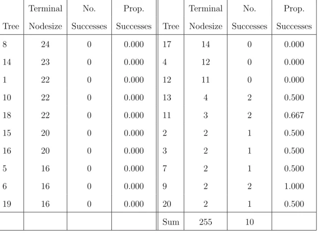
We begin by illustrating a situation in which the two aggregation schemes result in consid-erably different probability estimates. Since our intent for this section is to study differences in aggregation approaches, we only consider trees grown by the cForestpartitioning tech-nique. We simulated a training set of sizen= 100 from model (2.11) withβ0 =−2, and grew a small forest of 20 trees, using tuning parameters mtry=2, minsplit=5, and minbucket=1. We then made a prediction for a single new case with x1 = 0.6207, x2 = 1.8119, x3 = 1.9120, x4 =−1.3638. Table2.1 shows a summary of the terminal nodes containing the new case for each of the 20 trees.
Table 2.1: A summary of the terminal nodes containing a new case in a forest of 20 trees. The largest terminal nodes are the ones containing large numbers of training cases in the majority class. Table entries are ordered by terminal nodesize from largest to smallest.
Terminal No. Prop. Terminal No. Prop.
Tree Nodesize Successes Successes Tree Nodesize Successes Successes
8 24 0 0.000 17 14 0 0.000 14 23 0 0.000 4 12 0 0.000 1 22 0 0.000 12 11 0 0.000 10 22 0 0.000 13 4 2 0.500 18 22 0 0.000 11 3 2 0.667 15 20 0 0.000 2 2 1 0.500 16 20 0 0.000 3 2 1 0.500 5 16 0 0.000 7 2 1 0.500 6 16 0 0.000 9 2 2 1.000 19 16 0 0.000 20 2 1 0.500 Sum 255 10
The largest nodes containing this test case are all pure nodes and consist of cases from the majority class. The estimated success probabilities for the new case arePbEW(y∗ = 1)≈
0.2083, andPbP W(y∗ = 1) = 25510 ≈0.0392. Note that PbP W(y∗ = 1) is considerably lower as a
consequence of the trees with large, pure terminal nodes receiving more weight than those with small terminal nodes in the calculation of this estimate. Based on model (2.11), the true success probability is 1+exp(exp(−−2+02+0.6207).6207) ≈0.2011.
The preceding example is intended merely for illustrative purposes. In practice, forests much larger than 20 trees should be grown, and their performance needs to be evaluated on
more than one test case. Still, the example shows that large, pure terminal nodes affect pro-portional tree aggregation more than they affect aggregation by equal weighting, potentially resulting in very different probability estimates in the classification setting. This is typically not a concern in regression, as the response variable takes on many different values, allowing splitting to continue into approximately equally sized terminal nodes.
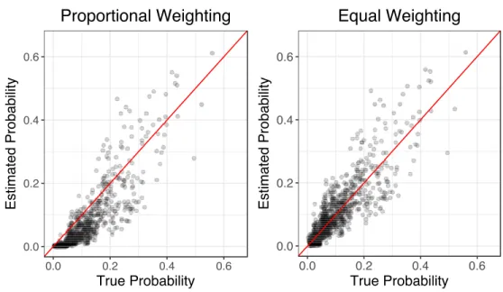
To further investigate the calibration of estimates produced by each aggregation ap-proach, we simulated a training set of size 10,000 from model (2.11), using a value of β0 = −2.564. This value was selected to create a dataset with an average true success probability of approximately 0.1. A random forest, consisting of 500 trees, was grown using
cForest with default paramter settings of minsplit = 20, and minbucket = 7. The mtry parameter was set to 2. Figure 2.1 displays the probability estimates, plotted against the true probabilities, determined from model (2.11).
0.0 0.2 0.4 0.6 0.0 0.2 0.4 0.6 True Probability Estimated Probability Proportional Weighting 0.0 0.2 0.4 0.6 0.0 0.2 0.4 0.6 True Probability Estimated Probability Equal Weighting 0.0 0.2 0.4 0.6 0.0 0.2 0.4 0.6 True Probability Estimated Probability Proportional Weighting 0.0 0.2 0.4 0.6 0.0 0.2 0.4 0.6 True Probability Estimated Probability Equal Weighting
Figure 2.1: Probability estimates using equal and proportional weighting for the aggregation of tree predictions and defaultcForestparameter settings,minsplit = 20 andminbucket= 7.
We see in Figure 2.1 that proportional aggregation typically underestimates the success probabilities. This is especially true for cases whose true success probabilities are less than 0.1, which constitute the majority of the test cases. The smaller than expected probabilities are the result of large pure terminal nodes in trees yielding a success probability estimate of 0, heavily influencing the proportionally weighted probability estimates. On the other hand, the equally weighted approach results in estimates that do not appear to be systematically too high or too low. In fact, the mean success probability for the 1,000 test cases was 0.0984, from model (2.11). The mean estimated success probability from proportional weighting is a substantially lower 0.0619, while the mean estimate, resulting from equal weighting, was 0.0994, which is right on target. Depending on the application at hand, underestimating the risk of a rare event by almost 4 percentage points can result in significant losses.
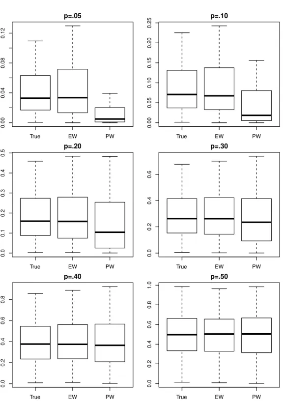
The values of β0 used in the preceding examples were selected in order to produce a dataset with far more failures than successes. In the literature, problems where one outcome is much more likely than another are referred to as as unbalanced classification problems. As is seen in Table 2.1, the pure terminal nodes that predict a failure are much larger than the pure terminal nodes that predict a success. A natural question is how the degree of imbalance affects probability estimates. To examine this question, values ofβ0, given in Table
2.2, were chosen to create datasets based on model (2.11) with mean success probabilities set to p = 0.05, p = 0.10, p = 0.20, p = 0.30, p = 0.40, and p = 0.50. To get a clear sense of the distribution of conditional probability estimates, we simulated 10,000 cases for both the training and test data. The same values ofX1,X2, X3, andX4 were used for each value of β0. Due to randomness, the true proportions of successes in the training and test sets vary slightly from the selected values of p (see Table 2.2). Random forests, consisting of 500 trees, were grown using defaultcForestparameter settings forminsplit and minbucket, and also using minbucket = minsplit = 1 to grow trees of maximal depth. We continue to
use mtry = 2. Based on the simulated data sets and random forests grown, we obtained probability estimates using each aggregation scheme.
Table 2.2: In the Bernoulli response example the proportion of successes in each training and test set for different imbalance ratios. Due to random variability, these differ slightly from the expected success probability, given by p.
β0 p Train Prop. Test Prop. -3.371 0.05 0.0541 0.0496 -2.564 0.10 0.1066 0.1026 -1.650 0.20 0.2002 0.1978 -1.018 0.30 0.3030 0.2983 -0.490 0.40 0.3994 0.3953 0 0.50 0.5049 0.5021
Figure 2.2 displays boxplots of the distributions of the true success probabilities, from model (2.11), and estimated probabilities for each imbalance ratio, using default cForest
settings, for both equal (EW) and proportional (PW) aggregation. It is immediately ap-parent that the median PW probability estimate is consistently less than the true median probability, while the distribution of EW estimates closely resembles the distribution of true probabilities. For PW, the extent of the difference appears to be related to the size of the imbalance between probability of success and failure.
True EW PW 0.00 0.04 0.08 0.12 p=.05 True EW PW 0.00 0.05 0.10 0.15 0.20 0.25 p=.10 True EW PW 0.0 0.1 0.2 0.3 0.4 0.5 p=.20 True EW PW 0.0 0.2 0.4 0.6 p=.30 True EW PW 0.0 0.2 0.4 0.6 0.8 p=.40 True EW PW 0.0 0.2 0.4 0.6 0.8 1.0 p=.50
Figure 2.2: Distribution of true and estimated probabilities using various degrees of imbal-ance and the default cForest terminal nodesize parameter settings of minsplit = 20 and minbucket= 7.
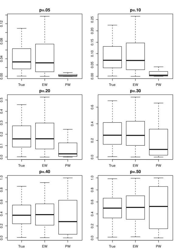
While concerns stemming from proportional weighted averaging are most obvious in unbalanced situations, it is inappropriate to dismiss this concern in more balanced settings. We see in Figure 2.2 that as the data become more balanced, and the distribution of PW estimates becomes more appropriately centered, it still exhibits more variability than the distribution of true probabilities. The increased spread is a result of the PW estimates being pulled toward the extremes by large pure nodes. This issue becomes more apparent when trees of maximal depth are grown, as is seen in Figure 2.3. Even for p = 0.5, large pure terminal nodes influence PW predictions heavily, pulling the probability estimates for cases more likely to result in successes toward 1 and for cases more likely to result in failure toward 0. In either case PW estimates lead to underestimation of the uncertaintly associated with a prediction.
Figures 2.2 and 2.3 suggest that problems arising from the PW aggregation scheme are more severe when trees of maximal depth are grown. Intuitively speaking, the sizes of large pure terminal nodes are unaffected by parameters restricting terminal nodesize, while nodes that are allowed to be small are given less weight, allowing the large pure terminal nodes to dominate PW probability estimate. While this suggests that we might be able to improve PW predictions by specifying large values for minsplit and minbucket, a downside is that an increase in these values might increase bias in tree predictions, which would be based on a large number of training cases, rather than just those most similar to the case being predicted. We address this topic in more detail in Section 2.4.
True EW PW 0.00 0.04 0.08 0.12 p=.05 True EW PW 0.00 0.05 0.10 0.15 0.20 0.25 p=.10 True EW PW 0.0 0.1 0.2 0.3 0.4 0.5 p=.20 True EW PW 0.0 0.2 0.4 0.6 p=.30 True EW PW 0.0 0.2 0.4 0.6 0.8 1.0 p=.40 True EW PW 0.0 0.2 0.4 0.6 0.8 1.0 p=.50
Figure 2.3: Distribution of true and estimated probabilities using various degrees of imbal-ance and terminal nodesize parameter settings of minsplit=minbucket= 1.
2.4
Data Applications
We have seen that aggregating tree predictions using a weighted average of tree pro-portions, as is done in cForest, potentially results in overestimation of the probability of the most likely response. This is especially a concern when working with unbalanced data. Possible remedies include requiring large terminal nodesizes, or weighting each tree equally when averaging. In this section, we explore the performance of the EW and PW aggregation approaches as well as the impact of increasing terminal nodesize using two real datasets in which class probability estimation is of interest.
The first dataset we consider is the credit card default (CCD) (Yeh and Lien, 2009) dataset available in the UCI machine learning repository (Lichman, 2013). The dataset consists of observations on 30,000 credit card holders in Taiwan. The response is binary, indicating whether the holder defaulted on a payment. Among the 23 predictor variables are numeric and categorical ones. The number of defaulting credit card holders is 6,636, accounting for 22.12% of observations.
The second dataset contains information on 8,748 students who declared a major in science, technology, engineering, or mathematics (STEM) at the beginning of their first year at a large public university between Fall 2011 and Fall 2014. The response variable is again binary, indicating whether the student left a STEM major by the start of the second year of enrollment. Note that students who left the institution before the start of the second year are not included in the dataset. The 30 predictor variables include numerical variables, such as standardized test scores, and categorical variables, such as gender and type of STEM major (e.g. biological sciences, engineering, etc.). While the original dataset is larger, we only consider a subset of the data containing the 8,748 students with complete data. A total of 873 students (9.98%) left STEM majors during their first year.
We used cross-validation to assess the performance of each partitioning and aggregation technique. We randomly divided the CCD dataset into 10 folds, each of size 3,000. Each fold was withheld once, and random forests, consisting of 500 trees, were trained on the remaining 27,000 observations and used to predict the 3,000 withheld cases. An analagous procedure was applied to the STEM dataset, using 9 folds of equal size. We examine performance using the partitioning and aggregation approaches employed bycForestandrandomForest
(for regression), along with our proposed method of combining the cForest partitioning algorithm with the randomForest regression aggregation approach. Table 2.3 summarizes the partitioning and aggregation approaches we considered.
Table 2.3: A summary of the partitioning and aggregation approaches we considered. Method Partitioning Algorithm Aggregation Algorithm
cForest Permutation Tests Proportional Weighting
randomForest CART (Gini Index) Equal Weighting Combined Permutation Tests Equal Weighting
We evaluate the performance of each partitioning and aggregation algorithm based on various terminal nodesize settings (minsplit in cForest and nodesize in randomForest), which are given in Table 2.4. Because an initial exploration showed that the default 3:1 ratio of minsplit to minbucket is often optimal and results are largely insenstive to changes inminbucket, we kept the default ratio.
Predictions are evaluated using a log loss function, which for vectors of estimates bp and true responses Y, is defined as
L(pb,y) =− n X
i=1
wherepbi =P(Yb i = 1|xi). This loss function is a popular choice for evaluating class probability
estimators. It is a proper scoring rule in the sense that its expectation is minimized by letting
b
pi = P(Yi = 1|xi) for each i. Other proper scoring rules for class probability estimation
include Brier score, which is equivalent to sum of squared errors when the response variable is binary, and boosting loss (Buja et al., 2005).
Table 2.4: Values of tuning parameters considered using cross-validation. Parameter Values Considered for CCD Values Considered for STEM
mtry 4, 8, 16 3, 5, 10, 20
minsplit (or nodesize) 1, 10, 25, 50, 100, 1, 5, 10, 25, 50, 75, 100, 150, 200, 300, 500 200, 250, 300, 400, 500
For each of the three prediction methods, and each terminal nodesize, we determined the optimal mtry value by minimizing L(pb,y) on OOB cases. Since each test case is predicted exactly once, we expect the mean estimated credit card default probability and the mean estimated probability of leaving STEM to be close to 0.2212, and 0.0998, respectively, when averaging across all folds. Average probability estimates that differ from these suggest a calibration problem.
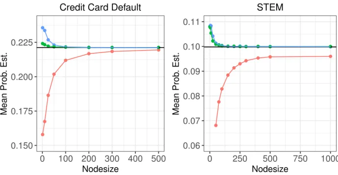
Figure2.4shows, as a function of terminal nodesize, the average estimated probability of a customer defaulting on credit card loans, or a student leaving STEM for each technique. We see that cForestseverly underestimates these probabilities when the terminal nodesize parameter is small. The disparity decreases as the terminal nodesize grows, but does not completely vanish. This behavior is especially pronounced in the STEM application, where even a terminal nodesize setting of 500 results in an average probability of leaving STEM that is about one-half of one percentage point lower than expected. Conversely therandomForest
defaulting on a loan, or leaving STEM when the terminal nodesize is small, but quickly converge to the proportions seen in the training data as nodesize grows.
0.150 0.175 0.200 0.225 0 100 200 300 400 500 Nodesize Mean Prob . Est.
Credit Card Default
0.06 0.07 0.08 0.09 0.10 0.11 0 250 500 750 1000 Nodesize Mean Prob . Est.
STEM
Method cForest Combined randomForest
Figure 2.4: The average estimated probability of default or leaving STEM is plotted against the value of the terminal nodesize parameter. The averagecForestestimates are consistently low, especially for small terminal nodesizes.
Figure2.5 shows the values of the log loss function on the holdout sets, averaging across folds. Plots (a) and (b) include a large enough range on the vertical axis to display all values, while plots (c) and (d) focus on regions of interest. The convex shape is consistent with the discussion of tuning parameters and model complexity in Section 2.2.3. We see that cForestperforms poorly when small terminal nodesize parameters are used, while the combined approach is less sensitive to small nodesizes. In the CCD dataset, the proposed approach achieves the best performance for each terminal nodesize, with a clear advantages
for small terminal nodesizes. In the STEM dataset, the cForestand combined approaches outperform randomForest. The combined approach performs best for terminal nodesizes less than 200, and is approximately equivalent to cForestfor terminal nodesize settings of 200 or greater. Optimal performance is obtained using nodesizes considerably larger than thancForestandrandomForestdefault values of 20 and 5, respectively. As nodesizes grow very large, performance deteriorates for all three methods.
1300 1350 1400 1450 1500 1550 0 100 200 300 400 500 Nodesize
Sum of Log Loss
Credit Card Default
a)
300 325 350 375 0 250 500 750 1000 NodesizeSum of Log Loss
STEM
b)
1280 1290 1300 1310 1320 0 100 200 300 400 500 NodesizeSum of Log Loss
Credit Card Default
c)
290 295 300 305 0 250 500 750 1000 NodesizeSum of Log Loss
STEM
d)
Method cForest Combined randomForest
Figure 2.5: The total log loss is plotted against the value of the terminal nodesize parameter. Figures (c) and (d) provide different versions of Figures (a) and (b), focusing the vertical axis on a narrower range.
Through Figures 2.4 and 2.5 we sought to study the performance of each algorithm as a function of nodesize. In practice, however, we are required to determine the appropriate nodesize parameter setting in addition to the mtry setting based on the OOB error in the
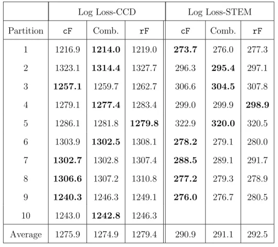
training data. Accordingly, we determined the best nodesize, mtry combination for each technique, within each fold, and used those values to obtain predictions for the holdout set. Table 2.5 gives the resulting log loss values on the holdout set for each partition, and each application. Values in boldface indicate the lowest log loss value among the three methods under consideration.
Table 2.5: Total log loss on each partition using cross validation for the CCD and STEM datasets.
Log Loss-CCD Log Loss-STEM
Partition cF Comb. rF cF Comb. rF
1 1216.9 1214.0 1219.0 273.7 276.0 277.3 2 1323.1 1314.4 1327.7 296.3 295.4 297.1 3 1257.1 1259.7 1262.7 306.6 304.5 307.8 4 1279.1 1277.4 1283.4 299.0 299.9 298.9 5 1286.1 1281.8 1279.8 322.9 320.0 320.5 6 1303.9 1302.5 1308.1 278.2 279.1 280.0 7 1302.7 1302.8 1307.4 288.5 289.1 291.7 8 1306.6 1307.2 1310.8 277.2 279.3 278.9 9 1240.3 1246.3 1249.1 276.0 276.7 280.5 10 1243.0 1242.8 1246.3 Average 1275.9 1274.9 1279.4 290.9 291.1 292.5
We see that the the permutation test based partitioning methods appear to achieve superior performance to CART, which is consistent with the claim that these techniques better utilize information provided by predictor variables that take on only a few values. Our combined method appears to achieve slightly more favorable performance on the CCD
dataset, while cForest performs slightly better in the STEM application. The differences between cForestand the combined approach are small.
The similar performance of cForest and our combined method is a result of the large terminal nodesize settings that are optimal in this problem. For the CCD dataset, the average terminal nodesizes, as determined using OOB log loss, were 140 for cForest, 150 for randomForest, and 120 for the combined method. For the STEM dataset, these values were 211.1, 83.3, and 130.6, respectively. However, applications can occur in which requiring large terminal nodes is undesirable.
Requiring large terminal nodes often prevents the separation of cases most likely to result in a credit card holder defaulting on a loan, or a student leaving STEM, from cases in which these outcomes are moderately likely. Suppose that the cost of failing to predict a credit card customer defaulting on a payment, or a student leaving STEM is higher than the cost of wrongly predicting such an occurrence. In these situations, a loss function that heavily penalizes failing to detect defaulting on a payment, or leaving STEM is appropriate. Let
Lα(pb,y) =− n X
i=1
[αI(Yi = 1)log(bpi) +I(Yi = 0)log(1−pbi)]
for α≥1. When it is especially important to accurately estimate probabilities for the cases carrying the highest risk (high P(Yi = 1) in our examples), this can be achieved by setting
α >1.
Table2.6shows how the average optimal terminal nodesize, determined using OOB error, changes as α increases, for each application. We see that the optimal terminal nodesize de-creases substantially for both randomForest and the combined approach. Smaller terminal nodesizes allow for splits that separate cases with very high risk, from those with moder-ately high risk, decreasing bias in probability estimates for the cases of greatest interest. However, optimal nodesizes increase for cForest. This results from the cForest
aggrega-tion scheme underestimating the probability of customer default or a student leaving STEM when nodesizes are allowed to be small. The cost of this underestimation outweighs the ben-efit of growing deeper trees, preventingcForestfrom taking advantage of finely partitioned training data.
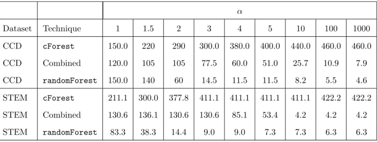
Table 2.6: Average terminal nodesize for each α, for the CCD and STEM datasets.
α Dataset Technique 1 1.5 2 3 4 5 10 100 1000 CCD cForest 150.0 220 290 300.0 380.0 400.0 440.0 460.0 460.0 CCD Combined 120.0 105 105 77.5 60.0 51.0 25.7 10.9 7.9 CCD randomForest 150.0 140 60 14.5 11.5 11.5 8.2 5.5 4.6 STEM cForest 211.1 300.0 377.8 411.1 411.1 411.1 411.1 422.2 422.2 STEM Combined 130.6 136.1 130.6 130.6 85.1 53.4 4.2 4.2 4.2 STEM randomForest 83.3 38.3 14.4 9.0 9.0 7.3 7.3 6.3 6.3
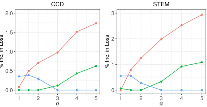
Figure 2.6 shows the percent increase in the Lα value incurred for each technique
com-pared to that of the optimal technique, for each value of α. As we observed previously, there is little difference between cForest and the combined approach when α = 1. How-ever, the relative performance of cForest begins to deteriorate quickly as α increases, due to its inability to finely partition training data without underestimating the probability of default or leaving STEM. For each dataset, the combined approach achieves the best perfo-mance for α = 1.5, and α = 2, and continues to outperform cForestfor larger α. In these applications, the randomForest algorithm performs best for large α. This is due to the fact that randomForest tends to overestimate the probability of default or leaving STEM when terminal nodesizes are small, as seen in Figure 2.4. There is no reason to believe that
randomForestis systematically likely to overestimate or underestimate the probability of an unlikely event in general, and its superior performance for large α is likely just an artifact
of these data. However, it is clear that the combined method is preferable to cForest for large α due to its ability to more accurately estimate probabilities for high-risk cases.
0.0 0.5 1.0 1.5 2.0 1 2 3 4 5 α % Inc. in Loss
CCD
0 1 2 3 1 2 3 4 5 α % Inc. in LossSTEM
Method cForest Combined randomForest
Figure 2.6: The percent of increase in loss for each technique relative to the best technique for a given penalty parameter α is plotted against α.
2.5
Conclusions
We have seen that random forests grown using conditional inference trees, implemented in the party package in R, are capable of achieving performance superior to those grown using the CART algorithm inrandomForest, especially in situations involving a mix of con-tinuous and categorical explanatory variables. We have further shown that the aggregation scheme employed by partytends to overestimate the probability of the most likely outcome,
a behavior that is especially prominent in unbalanced classification problems, though not restricted to this scenario.
When the depth of the trees is limited by use of a large minsplit value, the difference in performance between equally weighted tree aggregation and proportional weighting of trees is mostly negligible. When deep trees with small terminal nodes are desirable, equal weighting achieves superior performance to proportional weighting. The equal weighting aggregation scheme is less sensitive to changes in terminal nodesize settings than proportional weighting. This is a result of large, pure terminal nodes receiving disproportionate weight in proportional tree aggregation when when other nodes are allowed to be small. The appropriate teminal nodesize setting is context dependent, and careful use of cross-validation and OOB error when setting tuning paramters is essential.
In both data applications, trees grown incForestoutperform those grown inrandomForest. While cForest employs proportional weighting, it is possible to use equally weighted tree aggregation on random forests grown using cForest. In our applications, the performance of this combined approach is at worst on par withcForestand is better in some situations. We recommend using equally weighted tree aggregation in situations where deep trees with small terminal nodes are desirable, or when accurately estimating the mean success proba-bility for a large number of cases is important. If a dataset contains a mix of categorical and numerical predictor variables, then combining this aggregation scheme with thecForest par-titioning approach has the potential to produce better probability estimates than cForest
or randomForest individually. Combining the cForest partitioning approach with the re-gressionrandomForestaggregation technique allows users to take advantage of partitioning based on permutation tests and aggregation that is not disproportionately influenced by large pure terminal nodes, in order to more accurately estimate class probabilities.
Bibliography
Arpaci, A., Malowerschnig, B., Sass, O., and Vacik, H. (2014). Using multi variate data mining techniques for estimating fire susceptibility of tyrolean forests. Applied Geography, 53:258–270.
Breiman, L. (2001). Random forests. Machine Learning, 45(1):5–32.
Breiman, L. (2003). Manual—setting up, and understanding random forests V4.0.
Breiman, L., Friedman, J., Stone, C. J., and Olshen, R. A. (1984). Classification and regression trees. CRC press.
Buja, A., Stuetzle, W., and Shen, Y. (2005). Loss functions for binary class probability estimation and classification: Structure and applications. Working draft, November.
Bylander, T. (2002). Estimating generalization error on two-class datasets using out-of-bag estimates. Machine Learning, 48(1-3):287–297.
Hothorn, T., B¨uhlmann, P., Dudoit, S., Molinaro, A., and Van Der Laan, M. J. (2006a). Survival ensembles. Biostatistics, 7(3):355–373.
Hothorn, T., Hornik, K., and Zeileis, A. (2006b). Unbiased recursive partitioning: A condi-tional inference framework.Journal of Computational and Graphical Statistics, 15(3):651– 674.
Hothorn, T., Lausen, B., Benner, A., and Radespiel-Tr¨oger, M. (2004). Bagging survival trees. Statistics in Medicine, 23(1):77–91.
Janitza, S. (2017). On the overestimation of random forests out-of-bag error. Technical Report.
Liaw, A. and Wiener, M. (2002). Classification and regression by randomforest. R News, 2(3):18–22.
Lichman, M. (2013). UCI machine learning repository.
Meinshausen, N. (2006). Quantile regression forests. The Journal of Machine Learning Research, 7:983–999.
Mitchell, M. W. (2011). Bias of the random forest out-of-bag (oob) error for certain input parameters. Open Journal of Statistics, 2011.
R Core Team (2016). R: A Language and Environment for Statistical Computing. R Foun-dation for Statistical Computing, Vienna, Austria.
Sage, A. J. (2017). Github Repository.
Scott, S. B., Jackson, B. R., and Bergeman, C. (2011). What contributes to perceived stress in later life? a recursive partitioning approach. Psychology and Aging, 26(4):830.
Strobl, C., Boulesteix, A.-L., Kneib, T., Augustin, T., and Zeileis, A. (2008). Conditional variable importance for random forests. BMC Bioinformatics, 9(1):1.
Strobl, C., Boulesteix, A.-L., Zeileis, A., and Hothorn, T. (2007). Bias in random forest variable importance measures: Illustrations, sources and a solution. BMC Bioinformatics, 8(1):1.
Yeh, I.-C. and Lien, C.-h. (2009). The comparisons of data mining techniques for the pre-dictive accuracy of probability of default of credit card clients. Expert Systems with Ap-plications, 36(2):2473–2480.
CHAPTER 3.
RANDOM FOREST VARIABLE IMPORTANCE
IN THE PRESENCE OF MISSING DATA
A paper in preparation
Andrew J. Sage, Ulrike Genschel, and Dan Nettleton
Abstract
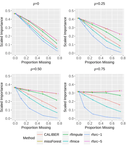
The ability to assess variable importance is a popular feature of random forest method-ology. Missing values in predictor variables are often imputed prior to making predictions and measuring variable importance. Numerous random-forest-based imputation techniques have been proposed. We assess the impact of these techniques on a random-forest-based measure of variable importance. After some imputation techniques are applied, the variable importance measure produces inflated estimates of importance for variables with many miss-ing observations. Other imputation techniques lead to deflated measures of importance for such variables. We compare the impact of six random-forest-based imputation techniques on measurements of variable importance, considering various possibilities for the number of missing values, and the correlation between predictor variables. Our work provides guidance on the choice of imputation technique for researchers who are interested in assessing variable importance when missing values are a concern.
3.1
Introduction
Random forest methodology is a nonparametric machine learning approach that uses recursive partitioning to make predictions in classification and regression problems. Random forests routinely handle situations where it is difficult to specify a parametric model because of many predictor variables, unknown nonlinear relationships between the predictors and the response, unknown high-order interactions, or a variety of other model complexities.
An important feature of random forest methodology is its ability to measure the impor-tance of predictor variables, which is often of interest in model selection or interpretation. Measuring variable importance can be challenging when a dataset contains missing values, especially if certain predictor variables are more prone to missingness than others. Complete case analysis, in which cases with missing values are ignored altogether, is widely considered a poor choice as it discards potentially useful information. When data are missing, researchers are likely to be interested in knowing which predictor variables would be most important in predicting a response if the data could have been fully observed. This information might, for example, be used to justify an increased effort to collect additional data on the most important predictors.
Missing values are often imputed prior to making predictions. Multiple imputation, a process by which missing values are imputed repeatedly in order to obtain several imputed datasets, is a popular approach that allows for an assessment of the variability associated with imputation. Numerous imputation approaches that make use of random forests are available (e.g. Breiman (2001); Ishwaran et al. (2008); Stekhoven and B¨uhlmann (2012); Doove et al. (2014); Shah et al. (2014)). Ideally, the measure of a predictor variable’s importance should not be affected by missingness and subsequent imputation. That is, the estimated importance of a predictor variable, when measured on the imputed dataset,
should be approximately the same, relative to other variables, as the importance estimate that would have been obtained if the complete data were available.
Numerous random-forest-based variable importance measures have been discussed in the literature. Most prominant is permutation importance (Breiman, 2003), which measures the loss in predictive accuracy when values for a predictor variable are randomly permuted. A less prominent measure, Gini Importance, (Breiman, 2001) determines the net decrease in impurity resulting from splits on a given predictor variable for classification problems. For datasets with missing values, Hapfelmeier et al. (2014b) developed an alteration to permutation importance that randomly allocates cases to nodes, rather than permuting values whenever a split is performed on the variable whose importance is being measured. Strobl et al. (2008) demonstrate that when permutation importance is used, variables that are correlated with important predictors tend to be considered important themselves, even if they do not add any new information beyond that provided by the correlated variable. Strobl et al. (2008) introduce a conditional variable importance measure that is intended to measure the value of adding a predictor variable when all other predictors are already included.
In the literature, there has been considerable attention given to developing random-forest-based imputation techniques and assessing the quality of the resulting imputed values. Tang and Ishwaran (2017) assess the performance of random-forest-based imputation techniques, finding these approaches to be generally robust. However, little attention has been given to the effect of imputation on measures of variable importance. Hapfelmeier et al. (2014b) in-troduce a self-contained variable importance measure that results from random forests grown in a way that handles missing values automatically. However, this procedure is intended to reflect the importance of a predictor variable given the data present, and missing observa-tions negatively impact a predictor variable’s importance estimate. When the objective is to assess the importance of a predictor variable if the variable had been able to be observed
completely, Hapfelmeier et al. (2014a) recommend using imputation prior to assessing vari-able importance, and present a case study comparing the results of one popular imputation technique to those obtained using their self-contained measure and a complete case analysis. In this study, we assess the impact of six random-forest-based imputation techniques on Breiman’s popular permutation importance measure of variable importance. Our objective is to assess the impact of imputation on the measure of an explanatory variable’s importance, rather than assessing the accuracy of the imputed values themselves, as is done by Tang and Ishwaran (2017). We demonstrate that some imputation techniques lead to a reduction in the estimated importance of variables with many missing values, while other techniques, somewhat paradoxically, result in inflated estimates of importance for such variables. In-flated estimates of variable importance can be especially problematic, as they might lead a researcher to incorrectly conclude that an unimportant variable with many missing values is important.
We structure the remainder of the manuscript in the following way. In Section 3.2, we provide a description of the popular random forest permutation importance measure, an overview of missing value terminology, and summaries of each imputation technique considered. In Section 4.4.1, we present a simulation study that demonstrates the effect of each imputation technique on the permutation variable importance measure, accounting for different proportions of missingness and various correlations between predictor variables. In Section 3.4, we analyze the effect of imputation on the permutation variable importance measure using real datasets in which variable importance is likely to be of interest. Finally, we summarize our conclusions in Section 3.5.
3.2
Variable Importance and Missing Values
3.2.1 Permutation Importance
We begin this section with a discussion of the permutation variable importance measure. In a random forest, each tree is typically grown using a bootstrap sample of the training data, so some cases are not used in the process of growing any given tree. These are known as out-of-bag (OOB) cases and are useful for assessing predictive performance and variable importance.
Let Ot be the subset of indices corresponding to the OOB cases for tree t, and let I(·)
denote a generic indicator function. Let | · | denote the number of elements in a set. The process of calculating the variable importance for a predictor variableXj can be summarized
in the following steps.
1. Grow a random forest on the set of training data. 2. For t = 1. . . , T, perform the following steps.
(a) For each i ∈Ot, predict the response for case i using tree t. Call this prediction
ˆ yit.
(b) For a regression problem, calculate MSEt = |O1t| X i∈Ot (yi−yˆit)2. For classification problems, calculate MCRt = |O1t| X i∈Ot I(yi 6= ˆyit).
(c) Randomly permute the values of Xj for all OOB cases and predict OOB cases
again. Call these predictions ˆy(itp).
(d) For a regression problem, calculate MSE(tp)= |O1
t| X i∈Ot (yi−yˆ (p) it ) 2.For classification problems, calculate MCR(tp)= |O1 t| X i∈Ot I(yi 6= ˆy (p) it ).
(e) Calculate the difference in predictive performance, Dt= MSE
(p)
t −MSEt or Dt=
3. Average the values obtained in (2e) across all trees to obtain a overall variable impor-tance score for Xj equal to T1
T X
t=1
Dt.
If permuting the values does not harm predictive performance, then Xj is considered
unimportant. On the other hand, if prediction accuracy decreases substantially, i.e. mean square error increases substantia