Full Terms & Conditions of access and use can be found at
http://www.tandfonline.com/action/journalInformation?journalCode=tssc20
Download by: [Cranfield University] Date: 08 July 2016, At: 03:24
Systems Science & Control Engineering
An Open Access Journal
ISSN: (Print) 2164-2583 (Online) Journal homepage: http://www.tandfonline.com/loi/tssc20
Nonlinear process fault detection and
identification using kernel PCA and kernel density
estimation
Raphael Tari Samuel & Yi Cao
To cite this article: Raphael Tari Samuel & Yi Cao (2016) Nonlinear process fault detection and identification using kernel PCA and kernel density estimation, Systems Science & Control Engineering, 4:1, 165-174, DOI: 10.1080/21642583.2016.1198940
To link to this article: http://dx.doi.org/10.1080/21642583.2016.1198940
© 2016 The Author(s). Published by Informa UK Limited, trading as Taylor & Francis Group
Accepted author version posted online: 16 Jun 2016.
Published online: 28 Jun 2016. Submit your article to this journal
Article views: 41
View related articles
SYSTEMS SCIENCE & CONTROL ENGINEERING: AN OPEN ACCESS JOURNAL, 2016 VOL. 4, 165–174
http://dx.doi.org/10.1080/21642583.2016.1198940
Nonlinear process fault detection and identification using kernel PCA and kernel
density estimation
Raphael Tari Samuel and Yi Cao
Oil and Gas Engineering Centre, School of Water, Energy and Environment, Cranfield University, Cranfield, UK
ABSTRACT
Kernel principal component analysis (KPCA) is an effective and efficient technique for monitoring nonlinear processes. However, associating it with upper control limits (UCLs) based on the Gaussian distribution can deteriorate its performance. In this paper, the kernel density estimation (KDE) tech-nique was used to estimate UCLs for KPCA-based nonlinear process monitoring. The monitoring performance of the resulting KPCA–KDE approach was then compared with KPCA, whose UCLs were based on the Gaussian distribution. Tests on the Tennessee Eastman process show that KPCA–KDE is more robust and provide better overall performance than KPCA with Gaussian assumption-based UCLs in both sensitivity and detection time. An efficient KPCA-KDE-assumption-based fault identification approach using complex step differentiation is also proposed.
ARTICLE HISTORY
Received 4 March 2015 Accepted 4 June 2016
KEYWORDS
Fault detection and identification; process monitoring; nonlinear systems; multivariatestatistics; kernel density estimation 1. Introduction
There has been an increasing interest in multivariate statistical process monitoring methods in both academic research and industrial applications in the last 25 years
(Chiang, Russell, & Braatz,2001; Ge, Song, & Gao,2013;
Russell, Chiang, & Braatz,2000; Yin, Ding, Xie, & Luo,2014;
Yin, Li, Gao, & Kaynak,2015). Principal component
analy-sis (PCA) (Jolliffe,2002; Wold, Esbensen, & Geladi,1987)
is probably the most popular among these techniques. PCA is capable of compressing high-dimensional data with little loss of information by projecting the data onto a lower-dimensional subspace defined by a new set of derived variables (principal components (PCs))
(Wise & Gallagher,1996). This also addresses the problem
of dependency between the original process variables. However, PCA is a linear technique; therefore, it does not consider or reveal nonlinearities inherent in many real industrial processes (Lee, Yoo, Choi, Vanrolleghem, &
Lee,2004). Hence, its performance is degraded when it
is applied to processes that exhibit significant nonlinear variable correlations.
To address the nonlinearity problem, Kramer (1992)
proposed a nonlinear PCA based on auto-associative
neu-ral network (NN). Dong & McAvoy (1996) suggested a
nonlinear PCA that combined principal curve and NN. Their approach involved: (i) using principal curve method to obtain associated scores and the correlated data,
CONTACT Yi Cao y.cao@cranfield.ac.uk
(ii) using an NN model to map the original data into scores, and (iii) mapping the scores into the original vari-ables. Nonlinear PCA methods have also been proposed
by (Cheng & Chiu, 2005; Hiden, Willis, Tham, &
Mon-tague,1999; Jia, Martin, & Morris,2000; Kruger, Antory,
Hahn, Irwin, & McCullough,2005). However, most of these
methods are based on NNs and require the solution of a nonlinear optimization problem.
Scholkopf, Smola, & Muller (1998) proposed Kernel
PCA (KPCA) as a nonlinear generalization of the PCA. A number of studies adopting the technique for nonlin-ear process monitoring have also been reported in the
literature (Cho, Lee, Choi, Lee, & Lee,2005; Choi, Lee, Lee,
Park, & Lee,2005; Ge et al.2013). KPCA is performed in two
steps: (i) mapping the input data into a high-dimensional feature space, and (ii) performing standard PCA in the feature space. Usually, high-dimensional mapping can seriously increase computational time. This difficulty is addressed in kernel methods by defining inner products of the mapped data points in the feature space, then expressing the algorithm in a way that needs only the values of the inner products. Computation of the inner products in the feature space is then done implicitly in the input space by choosing a kernel that corresponds to an inner product in the feature space. Unlike NN-based methods, KPCA does not involve solving a nonlinear opti-mization problem; it only solves an eigenvalue problem.
© 2016 The Author(s). Published by Informa UK Limited, trading as Taylor & Francis Group.
This is an Open Access article distributed under the terms of the Creative Commons Attribution License (http://creativecommons.org/licenses/by/4.0/), which permits unrestricted use, distribution, and reproduction in any medium, provided the original work is properly cited.
In addition, KPCA does not require specifying the num-ber of PCs to extract before building the model (Choi et al.,2005).
Similar to the PCA, the Hotelling’sT2statistic and the
Qstatistic (also known as squared prediction error, SPE)
are two indices commonly used in KPCA-based process
monitoring. TheT2 is used to monitor variations in the
model space while theQstatistic is used to monitor
vari-ations in the residual space. In a linear method such as PCA, computation of the upper control limits (UCLs) of
T2andQstatistics is based on the assumption that
ran-dom variables included in the data are Gaussian. The
actual distribution ofT2andQstatistics can be analytically
derived based on this assumption. Hence, the UCLs can also be derived analytically. However, many real indus-trial processes are nonlinear. Even though the sources of randomness of these processes could be assumed as Gaussian, variables included in measured data are non-Gaussian due to inherent nonlinearities. Hence, adopt-ing UCLs for fault detection based on the multivariate Gaussian assumption in such processes is inappropri-ate and may lead to misleading results (Ge & Song, 2013).
An alternative solution to the non-Gaussian prob-lem is to derive the UCLs from the underlying proba-bility density functions (PDFs) estimated directly from
the T2 and the Q statistics via a non-parametric
tech-nique such as kernel density estimation (KDE). This approach has been suggested in various linear tech-niques, such as PCA (Chen, Wynne, Goulding, & Sandoz,
2000; Liang, 2005), independent component analysis
(Xiong, Liang, & Qian,2007), and canonical variate
anal-ysis (Odiowei & Cao, 2010). It is even more important
to adopt this kind of approach to derive meaningful UCLs for a nonlinear technique such as the KPCA. This is because the Gaussian-assumption-based UCLs for latent variables obtained through a nonlinear technique will not be valid at all. Unfortunately, this issue has not attracted enough attention in the literature. In this work, the KDE approach is adopted to derive UCLs for PCA and KPCA. Then, their fault detection performances in the Tennessee Eastman (TE) process are compared with their Gaussian-assumption-based equivalents. The results show that the KDE-based approaches perform better than their coun-terparts with Gaussian-assumption-based UCLs. The con-tributions of this work can be summarized as follows:
• To combine the KPCA with KDE for the first time to
show that it is not appropriate to use the Gaussian-assumption-based UCLs with a nonlinear approach such as the KPCA.
• To compare the robustness of KPCA–KDE and KPCA
associated with Gaussian-assumption-based UCLs.
• Propose an efficient KPCA-KDE-based fault
identifica-tion approach using complex step differentiaidentifica-tion. The paper is organized as follows. The KPCA algorithm, KPCA-based fault detection and identification, and the
KDE technique are discussed in Section2. Application of
the monitoring approaches to the TE benchmark process
is presented in Section3. Finally, conclusions drawn from
the study are given in Section4.
2. KPCA–KDE-based process monitoring
2.1. Kernel PCA algorithm
Givenmtraining samplesxk∈ n,k=1,. . .,m, the data
can be projected onto a high-dimensional feature space
using a nonlinear mapping, φ:xk∈ n→φ(xk)∈ F.
The covariance matrix in the feature space is then com-puted as CF = 1 m m j=1 φ(xj),φ(xj), (1)
whereφ(xj), forj=1,. . .mis assumed to have zero mean
and unit variance. To diagonalize the covariance matrix, we solve the eigenvalue problem in the feature space as
λa=CFa, (2)
whereλis an eigenvalue ofCF, satisfyingλ≥0, anda∈
Fis the corresponding eigenvector (a=0).
The eigenvector can be expressed as a linear combina-tion of the mapped data points as follows:
a=
m
i=1
αiφ(xi). (3)
Usingφ(xk)to multiply both sides of Equation (2) gives
λφ(xk),a = φ(xk),CFa. (4) Substituting Equations (1) and (3) in Equation (4) we have
λ m i=1 αiφ(xk),φ(xi) = 1 m m i=1 αi φ(xk), m j=1 φ(xj) φ(xj),φ(xi). (5)
Instead of performing eigenvalue decomposition directly
onCF in Equation (1) and finding eigenvalues and PCs,
we apply the kernel trick by defining anm×m(kernel)
matrix as follows:
[K]ij=Kij= φ(xi),φ(xj) =k(xi,xj) (6)
for alli,j=1,. . .,m. Introducing the kernel function of
the formk(x,y)= φ(x),φ(y)in Equation (5) enables the
SYSTEMS SCIENCE & CONTROL ENGINEERING: AN OPEN ACCESS JOURNAL 167
computation of the inner productsφ(xi),φ(xj)in the
feature space as a function of the input data. This pre-cludes the need to carry out the nonlinear mappings and the explicit computation of inner products in the feature
space (Lee et al.,2004; Scholkopf et al.,1998). Applying
the kernel matrix, we re-write Equation (5) as λ m i=1 αiKki= 1 m m i=1 αi m j=1 KkjKji. (7)
Notice thatk=1,. . .,m, and therefore, Equation (7) can
be represented as
λmKα=K2α. (8)
Equation (8) is equivalent to the eigenvalue problem
mλα=Kα. (9) Furthermore, the kernel matrix can be mean centred as follows:
Kctr=K−UK−KU+UKU, (10)
where U is anm×m matrix in which each element is
equal to 1/m. Eigen decomposition ofKctris equivalent
to performing PCA in F. This, essentially, amounts to
resolving the eigenvalue problem in Equation (9), which
yields eigenvectorsα1,α2,. . .,αmand the corresponding
eigenvaluesλ1≥λ2≥. . . λm.
Since the kernel matrix,Kctris symmetric, the derived
PCs are orthonormal, that is,
αi,αj =δi,j,(i,j=1, 2,. . .,m), (11)
whereδi,jrepresents the Dirac delta function.
The score vectors of the nonlinear mapping of
mean-centred training observationsxj,j=1,. . .,m, can then be
extracted by projectingφ(xj)onto the PC space spanned
by the eigenvectorsαk,k=1,. . .,m, zk,j= αk,(kctr) = m i=1 αk,iφ(xi),φ(xj). (12)
Applying the kernel trick, this can be expressed as
zk,j= m
i=1
αk,i[Kctr]i,j. (13)
2.2. Fault detection metrics
The Hotelling’sT2of thejth samples in the feature space
used for KPCA fault detection is computed as
Tj2=[z1,j,. . .,zq,j]−1[z1,j,. . .,zq,j]T, (14)
where zi,j, i=1,. . .,q represents the PC scores of the
jth samples,q is the number of PCs retained and −1
represents the inverse of the matrix of eigenvalues
cor-responding to the retained PCs. The control limit ofT2
can be estimated from its distribution. If all scores are of Gaussian distributions, then the control limit
correspond-ing to a significance level,α,Tα2can be derived from the
F-distribution analytically as
Tα2∼q(m−1)
m−q Fq,m−q,α, (15)
Fq,m−q,αis the value of theF-distribution corresponding
to a significance level,αwith degrees of freedomqand
m−qfor the numerator and denominator, respectively.
Furthermore, a simplified computation of the Q
-statistic has been proposed (Lee et al.,2004). For thejth
samples, Qj= ||φ(xj)− ˆφq(xj)||2= m i=1 z2i,j− q i=1 z2i,j. (16)
If all scores are of normal distributions, the control limit
of theQ-statistic at the 100(1−α)% confidence level can
be derived as follows (Jackson,1991):
Qα=θ1 Cαh0 √ 2θ2 θ1 + 1+θ2h0(h0−1) θ2 1 1/h0 , (17) whereθi=nj=q+1λij,(i=1, 2, 3),h0=1−2θ1θ3/3θ22,λi
are the eigenvalues, and Cα is the 100(1−α) normal
percentile.
The alternative method of computing control
lim-its directly from the PDFs of the T2 and Q statistics is
explained in the next section.
2.3. Kernel density estimation
KDE is a procedure for fitting a data set with a suitable smooth PDF from a set of random samples. It is used widely for estimating PDFs, especially for univariate
ran-dom data (Bowman & Azzalini,1977). The KDE is
applica-ble for theT2andQstatistics since both are univariate
although the process characterized by these statistics is multivariate.
Given a random variabley, its PDF g(y)can be
esti-mated from itsmsamples,yj,j=1,. . .,m, as follows:
g(y)= 1 mh m j=1 K y−yj h , (18)
whereKis a kernel function whilehis the bandwidth or
smoothing parameter. The importance of selecting the bandwidth and methods of obtaining an optimum value
are documented in Chen et al. (2000) and Liang (2005).
Integrating the density function over a continuous
range gives the probability. Thus, assuming the PDFg(y),
the probability ofyto be less thancat a specified
signifi-cance level,αis given by
P(y<c)=
c
−∞g(y)dy=α. (19)
Consequently, the control limits of the monitoring
statis-tics (T2andQ) can be calculated from their respective PDF
estimates: T2 α −∞g(T 2)dT2=α, (20) Qα −∞g(Q)dQ=α. (21) 2.4. On-line monitoring
For a mean-centred test observation,xtt, the
correspond-ing kernel vector,kttis calculated with the training
sam-ples,xj,j=1,. . .,mas follows:
[ktt]j=k(xj,xtt). (22)
The test kernel vector is then centred as shown below:
kctt=ktt−Ku1−Uktt+UKu1, (23)
whereu1=1/m[1,. . ., 1]T∈ m. The corresponding test
score vector,zttis calculated using
ztt,k = αk,(kctt) = m
i=1
αk,iφ(xi),φ(xtt). (24)
This can be re-written as
ztt,k= m i=1 αk,i[kctt]i. (25) In vector form, ztt =Akctt, (26) whereA=[α1,· · ·,αm].
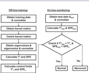
2.5. Outline of KPCA–KDE fault detection procedure
Tables1and2show the outline of KPCA–KDE-based fault
detection procedure.
To provide a more intuitive picture, a flowchart of the
procedure is presented in Figure1.
2.6. Fault variable identification
After a fault has been detected, it is important that the variables most strongly associated with the fault are iden-tified in order to facilitate the location of root causes.
Table 1.Off-line model development.
TR1. Obtain data under normal operating conditions (NOC) and scale the data using the mean and standard deviation of the columns of the data set which represent the different variables
TR2. Decide on the type of kernel function to use and determine the kernel parameter
TR3. Construct the kernel matrix of the NOC data and centre it using Equation (10)
TR4. Obtain eigenvalues and their corresponding eigenvectors and rearrange them in a descending order
TR5. Orthonormalize the eigenvectors using Equation (11) TR6. Obtain nonlinear components using Equation (13)
TR7. Compute monitoring indices(T2andQ) based on the kernelized NOC data using Equations (14) and (16)
TR8. Determine control limits ofT2andQusing Equations (20) and (21)
Table 2.On-line monitoring.
TT1. Acquire test sample xttand normalize using the mean and standard deviation values used in step 1 of the off-line stage
TT2. Compute the kernel vector of the test sample using Equation (22) TT3. Centre the kernel vector according to Equation (23)
TT4. Obtain the PC of the test sample from Equation (25)
TT5. Compare theT2andQof the test sample with their respective control limits obtained in the model development stage
TT6. If bothT2andQare less than their monitoring statistics, the process is in-control. If eitherT2orQexceeds its control limit, the process is out-of-control and therefore fault identification is carried out to identify the source of the fault
Figure 1.KPCA–KDE fault detection procedure.
Contribution plots which show the contributions of vari-ables to the high statistical index values in a fault region is a common method that is used to identify faults. How-ever, nonlinear PCA-based fault identification is not as straightforward as that of linear PCA due to the nonlinear relationship between the transformed and the original process variables.
In this article, fault variables were identified using a sensitivity analysis principle (Petzold, Barbara, Tech, Li,
Cao, & Serban,2006). The method is based on
calculat-ing the rate of change in system output variables resultcalculat-ing from changes in the problem causing parameters (Deng,
Tian, & Chen,2013). Given a test data vectorxi∈ nwith
SYSTEMS SCIENCE & CONTROL ENGINEERING: AN OPEN ACCESS JOURNAL 169
nvariables, the contribution of theithvariable to a
moni-toring index is defined by
Ti2,con=xiai and Qi,con=xibi, (27) whereai=∂T2/∂xiandbi=∂Q/∂xi. In this work, the par-tial derivatives were obtained by differentiating the
func-tions definingT2andQat a given reference fault instant
using complex step differentiation (Martins, Sturdza, &
Alonso,2003). This is an efficient generalized approach
for obtaining variable contributions in fault identification studies that use multivariate statistical methods.
3. Application
3.1. Tennessee Eastman process
The TE process is a simulation of a real industrial pro-cess manifesting both nonlinear and dynamic properties
(Downs & Vogel, 1993). It is widely used as a
bench-mark process for evaluating and comparing process
monitoring and control approaches (Chiang et al.,2001).
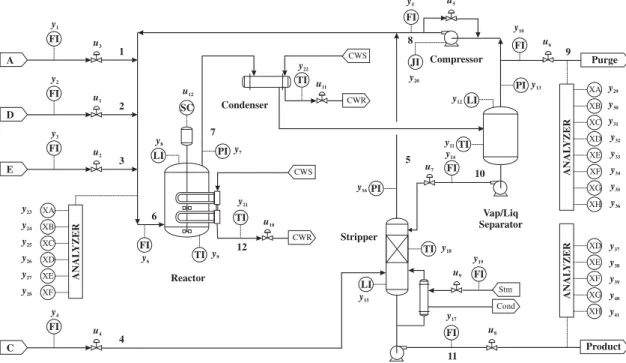
The process consists of five key units: separator, compres-sor, reactor, stripper and condenser, and eight compo-nents coded A to H. The control structure of the process
is presented in Figure2.
There are 960 samples and 53 variables, which include 22 continuous variables, 19 composition measurements sampled by 3 composition analysers, and 12 manipulated variables in the TE process. Sampling is done at 3-minute intervals while each fault is introduced at sample number 160. Information on disturbances and baseline operating
conditions of the process are documented in (Downs &
Vogel,1993; McAvoy & Ye,1994).
3.2. Application procedure
Five hundred samples obtained under NOC were used as the training data set and all 960 samples obtained under each of the faulty operating conditions were used as test data. All 22 continuous variables and 11 manipulated vari-ables were used in this study. The agitation speed of the reactor’s stirrer (the 12th manipulated variable) was not included because it is constant. A total of 20 faults in the process were studied. Descriptions of the variables and
faults studied are presented in Tables3and4.
Several methods have been proposed for determin-ing the number of retained PCs. Some of these methods are scree tests, the average eigenvalue approach, cross-validation, parallel analysis, Akaike information criterion, and the cumulative percent eigenvalue. However, none of these methods have been proved analytically to be the
best in all situations (Chiang et al.,2001). In this paper,
the number of PCs that explained over 90% of the total variance were retained. Based on this approach, 16 and 17 PCs were selected for PCA and KPCA, respectively.
Another, important parameter for kernel-based meth-ods in model development for process monitoring is the choice of kernel and its width. The radial basis kernel which is a common choice for process monitoring
stud-ies (Lee et al.,2004; Stefatos & Hamza,2007) was used
in this paper. The value of the kernel parameter c was
A FI y1 u3 1 D FI y2 u1 2 E FI y3 u2 C FI y4 u4 3 4 ANAL YZER XA y23 XB y24 XC y25 XD y26 XE y27 XF y28 SC LI FI TI PI Reactor CWR CWS TI Condenser CWS CWR TI Compressor FI JI LI TI FI TI LI Stripper Vap/Liq Separator Cond Stm FI FI Product ANAL YZER XD XE XF XG XH Purge ANAL YZER XD XC XB XA XE XF XG XH FI PI PI y37 y38 y39 y40 y41 y32 y33 y34 y35 y36 y29 y30 y31 y13 y10 y12 y20 y5 y11 y14 y18 y19 y17 y15 y16 y21 y9 y22 y7 y8 y6 u10 u11 u12 u5 u7 u9 u8 u6 7 6 12 8 5 11 10 9
Figure 2.Control structure of TE process.
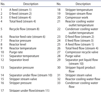
Table 3.TE process monitoring variables.
No. Description No. Description
1 A feed (stream 1) 18 Stripper temperature
2 D feed (stream 2) 19 Stripper stream flow
3 E feed (stream 4) 20 Compressor work
4 Total feed (stream 4) 21 Reactor cooling water
outlet temperature
5 Recycle flow (stream 8) 22 Condenser cooling water
outlet temperature 6 Reactor feed rate (stream 6) 23 D feed flow (stream 2)
7 Reactor pressure 24 E feed flow (stream 3)
8 Reactor level 25 A feed flow (stream 1)
9 Reactor temperature 26 Total feed flow (stream 4)
10 Purge rate 27 Compressor recycle valve
11 Separator temperature 28 Purge valve
12 Separator level 29 Separator pot liquid flow
(stream 10)
13 Separator pressure 30 Stripper liquid product
flow
14 Separator under flow (stream 10) 31 Stripper steam valve 15 Stripper stream valve 32 Reactor cooling water flow
16 Stripper pressure 33 Condenser cooling water
flow 17 Stripper under flow(stream 11)
Table 4.Fault descriptions in the TE process.
Fault Description Type
1 A/C feed ratio, B composition constant Step
2 B composition, A/C ratio constant Step
3 D feed temperature Step
4 Reactor cooling water inlet temperature Step 5 Condenser cooling water inlet temperature Step
6 A feed loss Step
7 C header pressure loss-reduced availability Step
8 A, B, C feed composition Random variation
9 D feed temperature Random variation
10 C feed temperature Random variation
11 Reactor cooling water inlet temperature Random variation 12 Condenser cooling water inlet temperature Random variation
13 Reaction kinetics Slow drift
14 Reactor cooling water valve Sticking
15 Condenser cooling water valve Sticking
16 Unknown
17 Unknown
18 Unknown
19 Unknown
20 Unknown
determined using the relation c=Wnσ2, where W is
a constant, which is dependent on the process being
monitored, n and σ2 are the dimension and variance
of the input space, respectively (Lee et al., 2004; Mika
et al.,1999). The value ofWwas set at 40 with validation
from the training data.
TheT2andQstatistics were used jointly for fault
detec-tion due to their complementary nature. This means that a fault detection was acknowledged when either of the monitoring statistics detected a fault. This is because detectable process variation may not always occur in both the model space and the residual space at the same time.
3.3. Fault detection rule
Since measurements obtained from chemical processes are usually noisy, monitoring indices may exceed their thresholds randomly. This amounts to announcing the presence of a fault when no disturbance has actually occurred, that is, a false alarm. In other words, a mon-itoring index may exceed its threshold once but if no fault is present, the monitoring index may not stay above its threshold in subsequent measurements. Con-versely, a fault has likely occurred if the monitoring index stays above its threshold in several consecutive measure-ments. A fault detection rule is used to address the
prob-lem of spurious alarms (Choi & Lee, 2004; Tien, Lin, &
Jun,2004; van Sprang, Ramaker, Westerhuis, Gurden, &
Smilde,2002). A detection rule also provides a uniform
basis for comparing different monitoring methods. In this paper, successful fault detection was counted when a monitoring index exceeds its control limit in at least two consecutive observations. All algorithms recorded a false alarm rate (FAR) of zero when tested with the training data based on this criterion. Computation of the met-rics for evaluating the monitoring performance of the different techniques was therefore based on this criterion.
3.4. Computation of monitoring performance metrics
Monitoring performance was based on three metrics: fault detection rates (FDRs), FARs, and detection delay. FDR is the percentage of fault samples identified cor-rectly. It was computed as
FDR= nfc
ntf ×
100, (28)
wherenfcdenotes the number of fault samples identified
correctly andntfis the total number of fault samples. FAR
was calculated as the percentage of normal samples iden-tified as faults (or abnormal) during the normal operation of the plant.
FAR=nnf
ntn ×
100, (29)
wherennfrepresents the number of normal samples
iden-tified as faults and ntn is the total number of normal
samples. Detection delay was computed as the time that elapsed before a fault introduced was detected.
3.5. Results and discussion
KPCA-based fault detection is demonstrated using Faults 11 and 12 of the TE process. Fault 11 is a random varia-tion in the reactor cooling water inlet temperature, while Fault 12 is a random variation in the condenser cooling
SYSTEMS SCIENCE & CONTROL ENGINEERING: AN OPEN ACCESS JOURNAL 171 Sample Number 0 200 400 600 800 1000 T 2 100 101 102 103 Sample Number 0 200 400 600 800 1000 SPE 10-4 10-3 10-2 10-1 100 Monitoring index Gaussian control limit KDE control limit
Figure 3.Monitoring charts for Fault 11.
Sample Number 0 200 400 600 800 1000 T 2 100 101 102 103 Sample Number 0 200 400 600 800 1000 SPE 10-4 10-3 10-2 10-1 100 Monitoring index Gaussian control limit KDE control limit
Figure 4.Monitoring charts for Fault 12.
water inlet temperature. The monitoring charts for the
two faults are shown in Figures3and 4, respectively. The
solid curves represent the monitoring indices, while the dash-dot and dash lines represent the control limits at 99% confidence level based on Gaussian distribution and KDE, respectively. It can be seen that in both cases,
espe-cially in theT2control charts, the KDE-based control limits
are below the Gaussian distribution-based control lim-its. That is, the monitoring indices exceed the KDE-based control limits to a greater extent compared to the Gaus-sian distribution-based control limits. This implies that using the KDE-based control limits with the KPCA tech-nique gives higher monitoring performance compared to using the Gaussian distribution-based control limits.
Table5shows the detection rates for PCA, PCA–KDE,
KPCA, and KPCA–KDE for all 20 faults studied. The results show that the KDE versions have overall higher FDRs
Table 5.Fault detection rates (%).
Fault PCA PCA–KDE KPCA KPCA–KDE
1 99.75 99.75 99.75 99.75 2 98.25 98.75 98.63 98.63 3 0.13 0.88 1.63 1.75 4 99.88 99.88 99.88 99.88 5 23.63 25.75 26.38 26.88 6 99.88 99.88 99.88 99.88 7 99.88 99.88 99.88 99.88 8 96.88 97.38 98.00 98.00 9 0.25 1.13 1.63 2.25 10 35.75 41.63 51.13 53.50 11 74.75 77.50 78.13 79.88 12 97.50 97.63 97.50 97.63 13 95.50 95.75 95.38 95.63 14 99.75 99.75 99.75 99.75 15 0 1.13 2.13 2.88 16 27.50 36.13 39.75 44.62 17 92.50 93.88 93.00 93.50 19 5.50 9.88 10.13 13.50 20 49.25 53.00 57.13 57.75
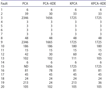
Table 6.Detection delay, DD (min).
Fault PCA PCA–KDE KPCA KPCA–KDE
1 6 6 6 6 2 39 30 33 33 3 2346 1656 1725 1725 4 3 3 3 3 5 3 3 3 3 6 3 3 3 3 7 3 3 3 3 8 48 48 48 48 9 2346 1665 1725 1725 10 186 186 180 180 11 15 15 15 15 12 42 30 60 42 13 102 102 111 105 14 6 6 6 6 15 ND 1656 1725 1725 16 81 78 81 81 17 45 45 45 45 18 24 24 24 24 19 213 24 213 36 20 105 102 105 105
Note: ND, not detected.
compared to the corresponding Gaussian
distribution-based versions. Furthermore, in Table6, it can be seen
that the detection delays of the KDE-based versions are either equal to or lower than the non-KDE-based tech-niques. This implies that the approaches based on KDE-derived UCLs detected faults earlier than their Gaussian distribution-based counterparts. Thus, associating KDE-based control limits with the KPCA technique for fault detection provides better monitoring compared to using control limits based on the Gaussian assumption.
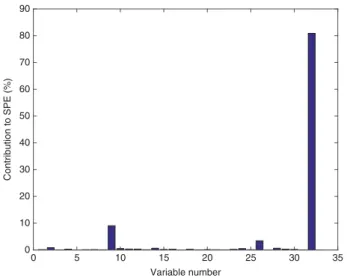
KPCA–KDE-based fault identification is demonstrated using Fault 11 as an example. The occurrence of Fault 11 induces change in the reactor cooling water flow rate, which causes the reactor temperature to fluctuate. Both
theT2- and SPE-based contribution plots at sample 300
shown in Figures5and6, respectively, identified the two
Variable number 0 5 10 15 20 25 30 35 Contribution to T 2 (%) 0 10 20 30 40 50 60
Figure 5.T2-based contribution plot for Fault 11.
Variable number 0 5 10 15 20 25 30 35 Contribution to SPE (%) 0 10 20 30 40 50 60 70 80 90
Figure 6.SPE-based contribution plot for Fault 11.
fault variables correctly. Variable 9 is the reactor tempera-ture while variable 32 corresponds to the reactor cooling water flow rate. Although it is possible for the control loops to compensate the change in the reactor temper-ature after a longer time has elapsed, the fluctuations in both variables affected early after the introduction of the fault were correctly identified by the contribution plots.
3.6. Test of robustness
To test the robustness of the KPCA–KDE technique, fault detection was performed by varying two parameters:
bandwidth and the number of PCs retained. Figure 7
shows the monitoring charts for KPCA and KPCA–KDE
with W=40 for Fault 14. This fault represents
stick-ing of the reactor coolstick-ing water valve, which is quit easily detected by most statistical process
monitor-ing approaches. AtW=40, both KPCA and KPCA–KDE
Sample Number 0 200 400 600 800 1000 T 2 101 102 103 Sample Number 0 200 400 600 800 1000 SPE 10-3 10-2 10-1 100 Monitoring index Gaussian control limit KDE control limit
Figure 7.KPCA-based control charts for Fault 14 atW=40 in the
formulac=Wnσ2. Sample Number 0 200 400 600 800 1000 T 2 100 101 102 103 Sample Number 0 200 400 600 800 1000 SPE 10-4 10-3 10-2 10-1 100 Monitoring index Gaussian control limit KDE control limit
Figure 8.KPCA–KDE-based control charts for Fault 14 atW=10
in the formulac=Wnσ2.
Table 7.Monitoring results at different number ofPCs retained.
KPCA KPCA–KDE PCs FDR FAR DD FDR FAR DD 10 99.88 0 3 99.88 0 3 15 99.75 0 6 99.75 0 6 20 96.75 0 6 99.88 0 3 25 99.88 8.13 3 99.75 0 6
recoded zero false alarms (Figure7). However, atW=10,
KPCA recorded a false alarm rate of 8.13% while the FAR
for KPCA–KDE was still zero (Figure8). Also, Table7shows
that the KPCA recorded a similar high FAR when 25 PCs were retained. Conversely, the KPCA–KDE approach still recorded zero false alarms.
Thus, apart from generally providing higher FDRs and earlier detections, the KPCA–KDE is more robust than the KPCA technique with control limits based on the
SYSTEMS SCIENCE & CONTROL ENGINEERING: AN OPEN ACCESS JOURNAL 173
Gaussian assumption. A more sensitive technique is bet-ter for process operators since less faults will be missed. Secondly, when faults are detected early, operators will have more time to find the root cause of the fault so that remedial actions can be taken before a serious upset occurs. Thirdly, although methods are available for obtaining optimum design parameters for developing process monitoring models, there is no guarantee that the optimum values are used all the time. The reason for this may range from lack of experience of personnel to lack of or limited understanding of the process itself. Therefore, the more robust a technique is, the better it is for process operations.
4. Conclusion
This paper investigated nonlinear process fault detec-tion and identificadetec-tion using the KPCA–KDE technique. In this approach, the thresholds used for constructing con-trol charts were derived directly from the PDFs of the monitoring indices instead of using thresholds based on the Gaussian distribution. The technique was applied to the benchmark Tennessee Eastman process and its fault detection performance was compared with the KPCA technique based on the Gaussian assumption.
The overall results show that KPCA–KDE detected faults more and earlier than the KPCA with control lim-its based on the Gaussian distribution. The study also shows that the UCLs based on KDE are more robust than those based on the Gaussian assumption because the former follow the actual distribution of the monitoring statistics more closely. In general, the work corroborates the claim that using KDE-based control limits give bet-ter monitoring results in nonlinear processes than using control limits based on the Gaussian assumption. A gen-eralizable approach for computing variable contributions in fault identification studies that centre on multivariate statistical methods was also demonstrated.
Disclosure statement
No potential conflict of interest was reported by the authors.
Funding
The first author was supported by Bayelsa State Scholarship Board (Government of Bayelsa State of Nigeria) [BSSB/AD/ CON/VOL.1 PHD.006].
References
Bowman, A. W., & Azzalini, A. (1977).Applied smoothing tech-niques for data analysis: The kernel approach with s-plus illus-trations. Oxford: Clarendon Press.
Chen, Q., Wynne, R. J., Goulding, P., & Sandoz, D. (2000). The application of principal component analysis and kernel den-sity estimation to enhance process monitoring.Control Engi-neering Practice,8(5), 531–543.
Cheng, C., & Chiu M.-S. (2005). Non-linear process monitoring using JITL-PCA.Chemometrics Intelligent Laboratory Systems, 76, 1–13.
Chiang, L., Russell, E., & Braatz, R. (2001).Fault detection and diagnosis in industrial systems. London: Springer-Verlag. Cho J.-H., Lee J.-M., Choi, S. W., Lee, D., & Lee I.-B. (2005). Fault
identification for process monitoring using kernel princi-pal component analysis.Chemical Engineering Science,60(1), 279–288.
Choi, S. W., & Lee I.-B. (2004). Nonlinear dynamic process mon-itoring based on dynamic kernel PCA.Chemical Engineering Science,59, 5897–5908.
Choi, S. W., Lee, C., Lee J.-M., Park, J. H., & Lee I.-B. (2005). Fault detection and identification of nonlinear processes based on kernel PCA.Chemometrics and Intelligent Laboratory Systems, 75, 55–67.
Deng, X., Tian, X., & Chen, S. (2013). Modified kernel prin-cipal component analysis based on local structure analy-sis and its application to nonlinear process fault diagno-sis.Chemometrics and Intelligent Laboratory Systems,127(15), 195–209.
Dong, D., & McAvoy, T. J. (1996). Non-linear principal component analysis-based on principal curves and neural networks.Computers and Chemical Engineering,20(1), 65–78.
Downs, J., & Vogel, E. (1993). A plant-wide industrial process control problem.Computers and Chemical Engineering,17(3), 245–255.
Ge, Z., & Song, Z. (2013). Multivariate statistical process con-trol: Process monitoring methods and applications. London: Springer-Verlag.
Ge, Z., Song, Z., & Gao, F. (2013). Review of recent research on data-based process monitoring.Industrial and Engineering Chemistry Research,52, 3543–3562.
Hiden, H. G., Willis, M. J., Tham, M. T., & Montague, G. A. (1999). Nonlinear principal component analysis using genetic pro-gramming.Computers and Chemical Engineering,23, 413–425. Jackson, J. (1991).A user’s guide to principal components. New
York, NY: Wiley.
Jia, F., Martin, E. B., & Morris, A. J. (2000). Non-linear princi-pal components analysis with application to process fault detection. International Journal of Systems Science, 31(11), 1473–1487.
Jolliffe, I. (2002). Principal component analysis (2nd ed). New York, NY: Springer-Verlag.
Kramer, M. A. (1992). Autoassociative neural networks. Comput-ers and Chemical Engineering,16(4), 313–328.
Kruger, U., Antory, D., Hahn, J., Irwin, G. W., & McCullough, G. (2005). Introduction of a nonlinearity measure for princi-pal component models.Computers and Chemical Engineering, 29(11–12), 2355–2362.
Lee J.-M., Yoo, C. K., Choi, S. W., Vanrolleghem, P. A., & Lee I.-B. (2004). Nonlinear process monitoring using kernel prin-cipal component analysis.Chemical Engineering Science,59, 223–234.
Liang, J. (2005). Multivariate statistical process monitoring using kernel density estimation. Developments in Chemical Engi-neering and Mineral Processing,13(1–2), 185–192.
Martins, J. R. R. A., Sturdza, P., & Alonso, J. J. (2003). The complex-step derivative approximation.ACM Transaction on Mathe-matical Software,29(3), 245–262.
McAvoy T. J., & Ye, N. (1994). Base control for the Tenessee Eastman problem.Computers and Chemical Engineering,18, 383–413.
Mika, S., Schölkopf, B., Smola, A., Müller, K. R., Scholz, M., & Rätsch, G. (1999). Kernel PCA and de-noising in feature spaces.Advances in Neural Information Processing System,11, 536–542.
Odiowei P. E. P., & Cao, Y. (2010). Nonlinear dynamic process monitoring using canonical variate analysis and kernel den-sity estimations.IEEE Transactions on Industrial Informatics, 6(1), 36–44.
Petzold, L., Barbara, S., Tech, V., Li, S., Cao, Y., & Serban, R. (2006). Sensitivity analysis of differential-algebraic equations and partial differential equations.Computers & Chemical Engi-neering,30(10–12), 1553–1559.
Russell, E., Chiang, L., & Braatz, R. (2000).Data-driven methods for fault detection and diagnosis in chemical processes. London: Springer-Verlag.
Schölkopf B., Smola, A. J., & Müller K.-R. (1998). Non-linear com-ponent analysis as a kernel eigenvalue problem.Neural Com-putation,10(5), 1299–1399.
van Sprang, E. N. M., Ramaker H.-J., Westerhuis, J. A., Gurden, S. P., & Smilde, A. K. (2002). Critical evaluation of approaches for
on-line batch process monitoring.Chemical Engineering Sci-ence,57(18), 3979–3991.
Stefatos, G., & Hamza, A. B. (2007).Statistical process control using kernel PCA. 15th Mediterranean Conference on Control and Automation, Anthens, Greece, 1418–1423.
Tien, D. X., Lin, K. W., & Jun, L. (2004).Comparative study of PCA approaches in process monitoring and fault detection. 30th Annual Conference on the IEEE Industrial Electronic Society, November 2-6, Busan Korea, 2594–2599.
Wise B. M., & Gallagher N . B. (1996). The process chemometrics approach to process monitoring and fault detection.Journal of Process Control,6, 329–348.
Wold, S., Esbensen, K., & Geladi, P. (1987). Principal compo-nent analysis.Chemometrics and Intelligent Laboratory Sys-tems,2(1–3), 37–52.
Xiong, L., Liang, J., & Qian, J. (2007). Multivariate statistical mon-itoring of an industrial polypropylene catalyser reactor with component analysis and kernel density estimation.Chinese Journal of Engineering,15(4), 524–532.
Yin, S., Ding, S. X., Xie, X. S., & Luo, H. (2014). A review on basic data-driven approaches for industrial process monitor-ing.IEEE Transactions on Industrial Electronics,61(11), 6418– 6428.
Yin, S., Li, X., Gao, H., & Kaynak, O. (2015). Data-based techniques focused on modern industry: An overview.IEEE Transactions on Industrial Electronics,62(1), 657–667.