Algorithms for Query-Efficient Active Learning

UC San Diego

UC San Diego Electronic Theses and Dissertations

Title

Algorithms for Query-Efficient Active Learning

Permalink https://escholarship.org/uc/item/6dq5q2t5 Author Yan, Songbai Publication Date 2019 Peer reviewed|Thesis/dissertation

UNIVERSITY OF CALIFORNIA SAN DIEGO Algorithms for Query-Efficient Active Learning A dissertation submitted in partial satisfaction of the

requirements for the degree Doctor of Philosophy in Computer Science by Songbai Yan Committee in charge:

Professor Kamalika Chaudhuri, Co-Chair Professor Tara Javidi, Co-Chair

Professor Sanjoy Dasgupta Professor Farinaz Koushanfar Professor Alon Orlitsky

Copyright Songbai Yan, 2019 All rights reserved.

The dissertation of Songbai Yan is approved, and it is accept-able in quality and form for publication on microfilm and electronically:

Co-Chair

Co-Chair

University of California San Diego

DEDICATION

EPIGRAPH

Nothing is more practical than a good theory.

TABLE OF CONTENTS

Signature Page . . . iii

Dedication . . . iv Epigraph . . . v Table of Contents . . . vi List of Figures . . . ix List of Tables . . . x Acknowledgements . . . xi Vita . . . xiii

Abstract of the Dissertation . . . xiv

Chapter 1 Introduction . . . 1

Chapter 2 Related Work . . . 7

2.1 Active Learning . . . 7

2.2 Efficient Learning of Halfspaces . . . 8

2.3 Interactive Models for Active Learning . . . 10

2.4 Learning with Observational Data . . . 11

Chapter 3 Preliminaries . . . 13

3.1 Learning Scenarios . . . 13

3.1.1 Stream-Based Active Learning . . . 14

3.1.2 Active Learning with Membership Queries . . . 14

3.2 Definitions . . . 15

3.3 The Disagreement-Based Active Learning Algorithm . . . 17

Chapter 4 Efficient Active Learning of Halfspaces with Bounded Noise . . . 19

4.1 Introduction . . . 19 4.2 Setup . . . 20 4.3 Algorithm . . . 22 4.4 Analysis . . . 24 4.4.1 Lower Bounds . . . 24 4.4.2 Upper Bounds . . . 31 4.5 Discussion . . . 42 4.5.1 Comparisons . . . 42

4.5.2 Implications to Passive Learning . . . 43

4.6 Acknowledgements . . . 45

Chapter 5 Active Learning with Abstention Feedback . . . 46

5.1 Introduction . . . 46

5.2 Setup . . . 47

5.2.1 Conditions for the Labeler . . . 49

5.3 Active Learning with Flat Abstention Rates . . . 51

5.3.1 Lower Bounds . . . 51

5.3.2 Algorithm and Analysis . . . 56

5.4 Active Learning with Monotonic Abstention Rates . . . 58

5.4.1 Algorithm . . . 59

5.4.2 Analysis . . . 62

5.4.3 Lower Bounds . . . 74

5.4.4 Remarks . . . 79

5.5 The Multidimensional Case . . . 80

5.5.1 Lower bounds . . . 80

5.5.2 Algorithm and Analysis . . . 86

5.6 Acknowledgements . . . 89

Chapter 6 Active Learning with Logged Observational Data I: An Importance Sam-pling Solution . . . 90 6.1 Introduction . . . 90 6.2 Setup . . . 92 6.3 Key Ideas . . . 94 6.4 Algorithm . . . 97 6.5 Analysis . . . 98 6.5.1 Consistency . . . 99 6.5.2 Label Complexity . . . 99 6.5.3 Remarks . . . 100 6.6 Experiments . . . 102 6.6.1 Methodology . . . 102 6.6.2 Implementation . . . 105

6.6.3 Results and Discussion . . . 107

6.7 Acknowledgements . . . 113

Chapter 7 Active Learning with Logged Observational Data II: A Solution with Re-duced Variance . . . 114

7.1 Introduction . . . 114

7.2 Variance-Controlled Importance Sampling . . . 116

7.2.1 Second-Moment-Regularized Empirical Risk Minimization 116 7.2.2 Clipped Importance Sampling . . . 119

7.3.1 Algorithm . . . 126

7.3.2 Analysis . . . 128

7.3.3 Discussion . . . 129

7.4 Acknowledgements . . . 131

Appendix A Omitted Proofs for Chapter 4 . . . 132

A.1 Basic Lemmas . . . 132

A.1.1 Basic Facts . . . 132

A.1.2 Probability Inequalities . . . 133

A.1.3 Properties of the Uniform Distribution over the Unit Sphere 134 A.2 Acute Initialization . . . 138

Appendix B Omitted Proofs for Chapter 5 . . . 141

B.1 Technical lemmas . . . 141

B.1.1 Concentration bounds . . . 141

B.1.2 Bounds of distances among probability distributions . . . . 144

B.1.3 Other lemmas . . . 149

Appendix C Omitted Proofs for Chapter 6 . . . 151

C.1 Preliminaries . . . 151

C.1.1 Summary of Key Notations . . . 151

C.1.2 Elementary Facts . . . 152

C.1.3 Facts on Disagreement Regions and Candidate Sets . . . 152

C.1.4 Facts on Multiple Importance Sampling Estimators . . . 153

C.2 Deviation Bounds . . . 156

C.3 Technical Lemmas . . . 160

C.4 Proof of Consistency . . . 164

C.5 Proof of Label Complexity . . . 165

Appendix D Omitted Proofs for Chapter 7 . . . 167

D.1 Preliminaries . . . 167

D.1.1 Summary of Key Notations . . . 167

D.1.2 Elementary Facts . . . 169

D.1.3 Facts on Disagreement Regions and Candidate Sets . . . 169

D.1.4 Facts on Multiple Importance Sampling Estimators . . . 170

D.1.5 Facts on the Sample Selection Bias Correction Query Strategy 171 D.1.6 Lower Bound Techniques . . . 173

D.2 Deviation Bounds . . . 173

D.3 Technical Lemmas . . . 178

D.4 Proofs for Section 7.3.2 . . . 181

D.5 Proofs for Sections 7.2 . . . 184

LIST OF FIGURES

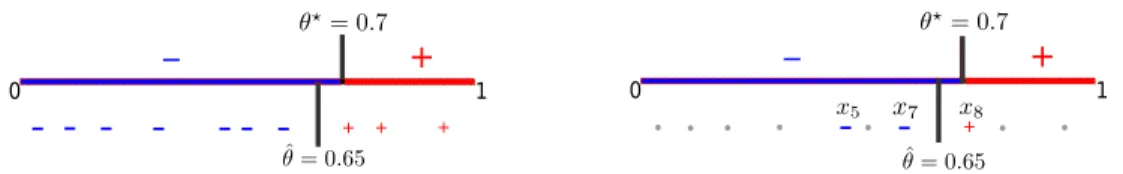
Figure 1.1: An example of learning a thresholdθ?=0.7 withn=10 unlabeled instances.

Left: in supervised learning, all labels are requested, and a threshold ˆθ=0.65

is returned; Right: in active learning, the learner sequentially queriesx₅,x₈,

x7, and returns ˆθ=0.65. Other instances (gray dots) are not queried. . . 2

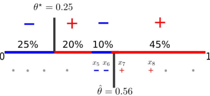
Figure 1.2: An example of learning thresholds in the non-realizable case. The best threshold is θ?=0.25 with error rate 0.1. In active learning, the learner sequentially queriesx5,x8,x7,x6. Other instances (gray dots) are not queried, and a suboptimal threshold ˆθ=0.56 with error rate 0.21 is returned. . . 4

Figure 5.1: A classifier with boundary g(x˜) = (x1−0.4)2+0.1 for d =2. Label 1 is assigned to the region above, 0 to the below (red region) . . . 50

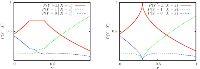
Figure 5.2: Left: The distributions satisfies Conditions 1 and 2, but the abstention feed-back is useless since P(_⊥|x) is flat between x=0.2 and 0.4. Right: The distributions satisfies Conditions 1, 2, and 3. The abstention feedback can be used to save queries. . . 51

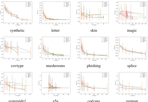
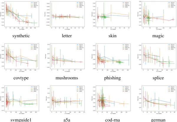
Figure 6.1: Test error vs. number of labels under the Identical policy . . . 109

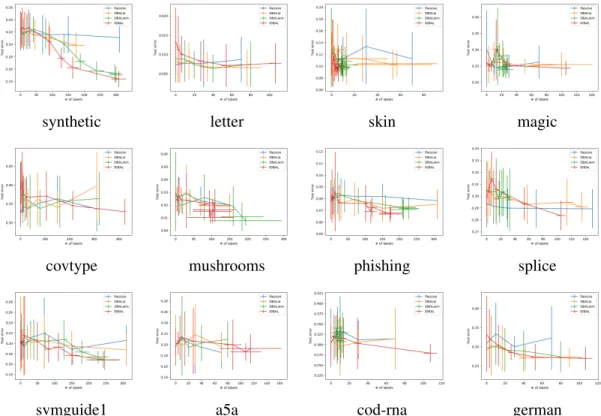
Figure 6.2: Test error vs. number of labels under the Uniform policy . . . 110

Figure 6.3: Test error vs. number of labels under the Uncertainty policy . . . 111

LIST OF TABLES

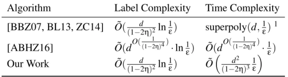
Table 4.1: A comparison of algorithms for active learning of halfspaces under the uniform

distribution, in theη-bounded noise model. . . 42

Table 4.2: A comparison of algorithms for PAC learning halfspaces under the uniform distribution, in theη-bounded noise model. . . 44

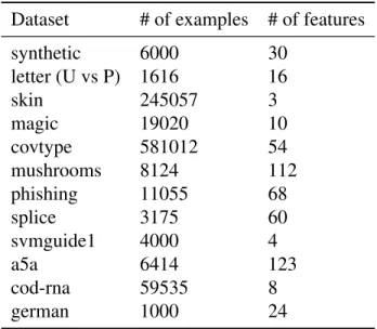
Table 6.1: Dataset information. . . 104

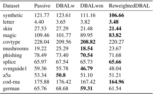
Table 6.2: AUC under Identical policy . . . 108

Table 6.3: AUC under Uniform policy . . . 110

Table 6.4: AUC under Uncertainty policy . . . 111

Table 6.5: AUC under Certainty policy . . . 112

ACKNOWLEDGEMENTS

I would like to express my deepest appreciation to my two wonderful advisors Professor Kamalika Chaudhuri and Professor Tara Javidi. I am indebted to them for their tolerance and continuous support over the past five years, for sharing their insights and knowledge, teaching me how to conduct and present my research, and offering life and career suggestions. I could not have imagined having a better advisor and mentor for my PhD study. I would like to thank the rest of my doctoral committee: Professor Sanjoy Dasgupta, Professor Farinaz Koushanfar, and Professor Alon Orlitsky, for their insightful comments and encouragement.

I was very fortunate to intern at Microsoft Research and Amazon AWS, which provides me with valuable industrial research experience. I am very grateful to my mentors Chris Meek and Sheeraz Ahmed for their kind guidance and inspiring discussions.

I want to thank my fellow colleagues at University of California San Diego: Julaiti Alafate, Akshay Balsubramani, Joseph Geumlek, Shuang Liu, Suqi Liu, Stefanos Poulis, Shuang Song, Christopher Tosh, Sharad Vikram, Mengting Wan, Xinan Wang, Yizheng Wang, Jiapeng Zhang, and many others, for the stimulating discussions and for all the fun we have had. I would particularly like to thank Chicheng Zhang, who gently shared his knowledge in learning theory and gave me enormous constructive comments and suggestions for my research.

I am grateful to my undergraduate advisor Professor Liwei Wang for enlightening me the first glance of machine learning research and offering me career guidance. My sincere thanks also go to my friends met at Peking University, Kai Fan, Chi Jin, Hongyi Zhang, from whom I learned a lot in our discussion and reading group.

Last but not least, I would like to thank my parents and my wife Linjie Peng, for supporting me spiritually throughout writing this dissertation and my life in general. This dissertation would not have been possible without them.

Chapter 4 is based on the material in Advances in Neural Information Processing Systems 2017 (Songbai Yan and Chicheng Zhang, “Revisiting perceptron: Efficient and label-optimal

active learning of halfspaces”). The dissertation author is the primary investigator and co-author of this material.

Chapter 5 is based on the materials in Allerton Conference on Communication, Control and Computing 2015 (Songbai Yan, Kamalika Chaudhuri and Tara Javidi, ”Active Learning from Noisy and Abstention Feedback”) and Advances in Neural Information Processing Systems 2016 (Songbai Yan, Kamalika Chaudhuri and Tara Javidi, ”Active Learning from Imperfect Labelers”). The dissertation author is the primary investigator and author of these materials.

Chapter 6 is based on the material in International Conference on Machine Learning 2018 (Songbai Yan, Kamalika Chaudhuri and Tara Javidi, ”Active Learning with Logged Data”). The dissertation author is the co-primary investigator and co-author of this material.

Chapter 7 is based on the material submitted to Advances in Neural Information Processing Systems 2019 (Songbai Yan, Kamalika Chaudhuri and Tara Javidi, ”The Label Complexity of Active Learning from Observational Data”). The dissertation author is the co-primary investigator and co-author of this material.

VITA

2014 B. S. in Computer Science and Technology, Peking University, China 2017 M. S. in Computer Science, University of California San Diego, USA 2019 Ph. D. in Computer Science, University of California San Diego, USA

PUBLICATIONS

Songbai Yan, Kamalika Chaudhuri and Tara Javidi, “Active Learning with Logged Data”, manuscript, 2019.

Varun Chandrasekaran, Kamalika Chaudhuri, Irene Giacomelli, Somesh Jha and Songbai Yan, “Exploring Connections Between Active Learning and Model Extraction”,manuscript, 2019.

Songbai Yan, Kamalika Chaudhuri and Tara Javidi, “Active Learning with Logged Data”, Inter-national Conference on Machine Learning, 2018.

Songbai Yan, Chicheng Zhang, “Revisiting Perceptron: Efficient and Label-Optimal Learning of Halfspaces”,Neural Information Processing Systems, 2017.

Songbai Yan, Kamalika Chaudhuri and Tara Javidi, “Active Learning from Imperfect Labelers”, Neural Information Processing Systems, 2016.

Songbai Yan, Kamalika Chaudhuri and Tara Javidi, “Active Learning from Noisy and Abstention Feedback”,Allerton Conference on Communication, Control and Computing, 2015.

ABSTRACT OF THE DISSERTATION

Algorithms for Query-Efficient Active Learning

by

Songbai Yan

Doctor of Philosophy in Computer Science

University of California San Diego, 2019

Professor Kamalika Chaudhuri, Co-Chair Professor Tara Javidi, Co-Chair

Recent decades have witnessed great success of machine learning, especially for tasks where large annotated datasets are available for training models. However, in many applications, raw data, such as images, are abundant, but annotations, such as descriptions of images, are scarce. Annotating data requires human effort and can be expensive. Consequently, one of the central problems in machine learning is how to train an accurate model with as few human annotations as possible. Active learning addresses this problem by bringing the annotator to work together with the learner in the learning process. In active learning, a learner can sequentially select examples and ask the annotator for labels, so that it may require fewer annotations if the learning algorithm

avoids querying less informative examples.

This dissertation focuses on designing provable query-efficient active learning algorithms. The main contributions are as follows. First, we study noise-tolerant active learning in the standard stream-based setting. We propose a computationally efficient algorithm for actively learning homogeneous halfspaces under bounded noise, and prove it achieves nearly optimal label complexity. Second, we theoretically investigate a novel interactive model where the annotator can not only return noisy labels, but also abstain from labeling. We propose an algorithm which utilizes abstention responses, and analyze its statistical consistency and query complexity under different conditions of the noise and abstention rate. Finally, we study how to utilize auxiliary datasets in active learning. We consider a scenario where the learner has access to a logged observational dataset where labeled examples are observed conditioned on a selection policy. We propose algorithms that effectively take advantage of both auxiliary datasets and active learning. We prove that these algorithms are statistically consistent, and achieve a lower label requirement than alternative methods theoretically and empirically.

Chapter 1

Introduction

Recent decades have witnessed great success of machine learning in various tasks, such as computer vision [RF17], natural language processing [VSP+17], and recommender sys-tems [MTSVDH15]. One of the key factors to this success is the availability of large-scale annotated datasets such as images with class labels and products with user reviews. However, in many applications, raw data, such as DNA sequences and medical images, are abundant, but annotating them requires domain expertise and can be expensive. Consequently, one of the central problems in machine learning is how to train an accurate model with as few human annotations as possible.

One solution to this problem is through active learning where the learner works together with the annotator during the learning process. In active learning, a learner can sequentially select examples and ask the annotator for labels, so that it may require fewer annotations if the learning algorithm avoids querying less informative examples. It has been shown that active learning indeed helps reduce labeling efforts effectively in many tasks in natural language processing [SYL+18], computer vision [KSH+16, LWD+19], recommender systems [ERR16, KRG18], etc.

0 1 + _ 0 1 + _

_

_ _

_

_ _ _

_{+ + +}

_

_

+

Figure 1.1: An example of learning a thresholdθ?=0.7 with n=10 unlabeled instances.

Left: in supervised learning, all labels are requested, and a threshold ˆθ=0.65 is returned;

Right: in active learning, the learner sequentially queriesx5,x8,x7, and returns ˆθ=0.65. Other instances (gray dots) are not queried.

How Active Learning Reduces Annotation Requirement

One classic example where active learning yields exponential label-efficiency improve-ment is learning a one-dimensional threshold with binary search. Consider a binary classification task where instances are real numbers from the unit interval [0,1], and the label can be either positive (+1) or negative (₋1). Assume there is a thresholdθ?∈[0,1]that perfectly separates

the data, that is, any examplexsmaller thanθ?is labeled negative and otherwise positive. To

learnθ?, in the standard supervised learning setting, as shown in Figure 1.1 (left), the learner

would first drawninstances and request labels for all of them, and then output a threshold ˆθthat

predicts correct labels for all observed instances. To guarantee_|θˆ−θ?| ≤ε, this passive learner

needsn=Ω(1_ε)labeled instances.

However, in the active learning setting, the learner could apply the binary search algorithm to find the threshold with much fewer labels. As shown in Figure 1.1 (right), the learner first drawsninstances, but only requests the label for the instance in the middle. If its label is negative (resp. positive), then the learner can infer that all instances on its left (resp. right) are negative (resp. positive) as well and only needs to recursively search forθ? in the right (resp. left) half

interval. In the end of this binary search procedure, the learner outputs a threshold ˆθthat predicts

correct labels for all observed instances. It is easy to see that to guarantee_|θˆ−θ?| ≤ε, this active

learner needs n=O(1_ε) unlabeled instances but only O(log1

ε)labels, which is exponentially

smaller than the label requirement for the passive learner.

general and widely used active learning algorithms, including generalized binary search [Now11] where instances that can rapidly narrow down the version space are selected are queried, margin-based methods [TK01, BBZ07] where examples near the current estimated boundary are queried, and disagreement based methods [CAL94, BBL06a] where examples are queried only if their labels cannot be confidently inferred.

How Active Learning Fails

Active learning is significantly more challenging in the nonrealizable case where no classifier in the hypothesis class achieves 100% accuracy. In this case, an improperly designed active learning algorithm may yield poor performance, mostly due to noisy annotations or sampling bias.

Noisy Annotations Human annotators can make mistakes, so the feedback returned to

the learner may not always be consistent with the underlying ground truth. If handled improperly, an incorrect label may divert the active learning algorithm from the correct boundary and lead to a classifier with a high error rate. To illustrate this, consider again the threshold learning task in Figure 1.1. If the annotator returns an incorrect label +1 upon the first queryx₅from the active learner, and if the learner still uses the standard binary search algorithm, then the learner would incorrectly believeθ?∈[0,x5], and recursively query in this half interval. Even if the annotator

makes no more mistakes afterward, the learner will output a threshold ˆθ≤0.5, which is far from

the ground truthθ?.

Sampling Bias An active learner often selects instances according to some criteria to

query for labels. As a result, the distribution of labeled instances observed by the learner can be different from the actual data distribution, which can result in suboptimal solution especially in the non-realizable case where no classifier in the hypothesis class perfectly predicts all labels. To

0 1

+

_

_

+

25% 20% 10% 45% +

_ _

₊

Figure 1.2: An example of learning thresholds in the non-realizable case. The best threshold is

θ?=0.25 with error rate 0.1. In active learning, the learner sequentially queriesx5,x8,x7,x6. Other instances (gray dots) are not queried, and a suboptimal threshold ˆθ=0.56 with error rate

0.21 is returned.

illustrate this, consider the threshold learning task as shown in Figure 1.2. We assume unlabeled instances are drawn uniformly from the unit interval and the corresponding ground truth labels are shown in the figure. In this example, no threshold function is 100% accurate, but we still want the algorithm to output a threshold as accurate as possible (in this example, the optimal threshold isθ?=0.25, which makes mistakes with probability 0.1). In supervised learning, the learner can

apply the Empirical Risk Minimization principle: it first drawsninstances, requests labels for all of them, and then outputs a threshold ˆθthat makes the fewest number of mistakes on observed

instances. It can be shown that this method isstatistically consistent, meaning that ˆθ→θ?as

n_→∞. However, the standard binary search algorithm for active learning is not statistically

consistent: with high probability, it first queries an instance x5 in the middle and receives a

negative label; subsequently it recursively queries in its right and finally returns a classifier around 0.55, which is far from the optimal thresholdθ?no matter how many labels are queried.

Hence, one main challenge in active learning is how to design query-efficient algo-rithms that tolerate mistakes of human annotators and guarantees statistical consistency. In the past decades, many active learning algorithms have been proposed and analyzed [CAL94, BBL06b, Han07, Das05, CN08, Now11, NJC15, CHK17, TD17, BBZ07, ABL14, ABHZ16, BDL09, BHLZ10, HAH+15]. In this dissertation, we investigate three directions to advance the research on provably query-efficient active learning: (1) designing noise-tolerant active learning

algorithms in the standard active learning setting; (2) exploring new interactive models beyond standard label feedback; (3) utilizing auxiliary information available to the learner.

Our Contributions

Efficient Active Learning of Halfspaces with Bounded Noise In Chapter 4, we study

noise-tolerant learning of halfspaces under the standard stream-based active learning setting. We propose a computationally efficient Perceptron-based algorithm for actively learning homoge-neous halfspaces under the uniform distribution over the unit sphere. We prove that under the bounded noise condition, where each label is flipped with probability at most 1₂, our algorithm achieves a near-optimal label complexity.

Active Learning with Abstention Feedback In Chapter 5, we study a new interactive

model where the annotator can not only return noisy labels, but also abstain from labeling. We consider different noise and abstention conditions of the annotator. We propose an algorithm which utilizes abstention responses. We prove this algorithm is statistically consistent and achieves nearly optimal query complexity under fairly natural conditions.

Active Learning with Logged Observational Data In the final two chapters, we study

how to utilize an auxiliary dataset in active learning. In particular, We consider a scenario where the learner has access to a logged observational dataset where labeled examples are observed conditioned on a selection policy. In Chapter 6, we apply multiple importance sampling to utilize the logged data in active learning effectively and introduce a novel debiasing policy that selectively avoids querying those examples that are highly represented in the logged observational data. We prove that our algorithm is statistically consistent, and has a lower label requirement

than alternatives both theoretically and empirically. In Chapter 7, we show how to apply variance control techniques to obtain a more sample-efficient error estimator, and then incorporate it into the active learning algorithm. We provably demonstrate that the new algorithm is statistically consistent as well as more label-efficient than the prior work.

Chapter 2

Related Work

2.1

Active Learning

In recent years, there has been extensive research in both theory and practice of active learning; see excellent surveys by [Set10, Das11, Han14]. On the theoretical side, many active learning algorithms have been proposed and analyzed. An incomplete list includes disagreement-based methods [CAL94, BBL06b, Han07], generalized binary search [Das05, CN08, Now11, NJC15, CHK17, TD17], margin-based methods [BBZ07, ABL14, ABHZ16], and importance weighted methods [BDL09, BHLZ10, HAH+15]. There is also a considerable amount of work on lower bounds of label complexity for active learning under various noise conditions, and refined algorithms and analysis that approach these lower bounds [Han09, Kol10, RR11a, ZC14, HY15]. However, most of these algorithms are computationally efficient as they require either explicit enumeration of classifiers in hypothesis classes, or solving empirical 0-1 loss minimization problems.

been proposed, including uncertainty sampling [LG94, TK01], query by committee [SOS92, FSST97], maximizing expected model change [SCR08], and encouraging sample diversity [NS04, SS18]. It has been shown that these heuristics help reduce labeling efforts effectively in many tasks in natural language processing [SYL+18], computer vision [KSH+16, LWD+19], recommender systems [ERR16, KRG18], etc.

In this dissertation, we advance the research on provably query-efficient active learning from three aspects: (1) we propose a label-optimal and computationally efficient active learning algorithm for learning halfspaces with bounded noise; (2) we explore a new interactive model that allows the annotator to abstain from labeling; (3) we show how to utilize an auxiliary observational dataset in active learning.

2.2

Efficient Learning of Halfspaces

Efficient learning of halfspaces is one of the central problems in machine learning [CST00]. In the realizable case, it is well known that linear programming finds a consistent hypothesis over data efficiently. In the nonrealizable setting, however, the problem is much more challenging.

A series of papers [ABSS93, FGKP06, GR09, KK14, Dan15] have shown the hardness of learning halfspaces with agnostic noise. The state of the art result [Dan15] shows that under standard complexity-theoretic assumptions, there exists a data distribution, such that the best linear classifier has erroro(1), but no polynomial time algorithms can achieve an error at most 1_2−d1c

for everyc>0, even with improper learning. [KK14] shows that under standard assumptions (learningk-sparse parity with noise must have timenΩ(k)_{), even if the unlabeled distribution is} Gaussian, any agnostic halfspace learning algorithm must run in time (1_ε)Ω(lnd) _{to achieve an} excess error ofε. These results indicate that, to have nontrivial guarantees on learning halfspaces

with noise in polynomial time, one has to make additional assumptions on the data distribution over instances and labels.

Since it is believed to be hard for learning halfspaces in the general agnostic setting, it is natural to consider algorithms that work under more moderate noise conditions. Despite consid-erable efforts, there are only a few halfspace learning algorithms that are both computationally-efficient and label-computationally-efficient. In the realizable setting, [DKM05, BBZ07, BL13] propose computa-tionally efficient active learning algorithms which have an optimal label complexity of ˜O(dln1

ε).

Under the bounded noise setting [MN06], the only known algorithms that are both label-efficient and computationally-efficient are [ABHU15, ABHZ16]. [ABHU15] uses a margin-based frame-work which queries the labels of examples near the decision boundary. To achieve computational efficiency, it adaptively chooses a sequence of hinge loss minimization problems to optimize as opposed to directly optimizing the 0-1 loss. It works only when the label flipping probability upper boundηis small (η≤1.8×10−6). [ABHZ16] improves over [ABHU15] by adapting a

polynomial regression procedure into the margin-based framework. It works for anyη<1/2, but

its label complexity isO(dO(

1

(1−2η)4)_ln1

ε), which is far worse than the information-theoretic lower

boundΩ(₍₁ d

−2η)2ln

1

ε). Recently [CHK17] gives an efficient algorithm with a near-optimal label

complexity under the membership query model where the learner can query on synthesized points. However, it is unclear how to transform the DC algorithm in [CHK17] into a computationally efficient stream-based active learning algorithm where the learner can only query on points drawn from the data distribution.

In Chapter 4, we provide a Perceptron-based algorithm that is computationally efficient and achieves nearly optimal label complexity for learning halfspaces under the bounded noise setting.

2.3

Interactive Models for Active Learning

In the standard active learning setting, the learner obtains labels from an annotator. Three interactive models between the learner and the annotator are commonly used: (1) the membership query model, where the learner can query any instances in the instance space for labels; (2) the stream-based query model, where the learner is presented a stream of unlabeled instances drawn from an underlying distribution one at a time, and for each of them the learner needs to decide whether to query for its label or not in an online fashion; (3) the pool-based query model, where the learner is presented a pool of unlabeled examples drawn from an underlying distribution, and it can iteratively query some of them for labels. In Chapter 5, we work with the membership query model. In Chapters 4, 6, and 7, we work with the stream-based query model. We note that an algorithm for the stream-based query model also works under the pool-based query model, while converting an algorithm from the pool-based model to stream-based model is nontrivial and there can be a significant gap with respect to label complexity under these two models [SH16].

Many novel interactive models are studied where annotators can provide information be-yond label feedback. For example, [Ang88, Heg95] consider equivalence query where the learner presents a classifier to the annotator, and the annotator either confirms this classifier is correct or otherwise returns a counter-example. [BH12] considers class-conditional query where the learner presents an unlabeled instance setU and a class label, and the annotator returns an example of classcfromU. [ZC15] considers a setting where the learner can choose to query for labels from a cheap but noisy annotator or an expensive but accurate one. [BHLZ16] considers search query where the learner presents a set of classifiersV, and the annotator returns a labeled example on which all classifiers inV predict incorrectly. [XZM+17] considers pairwise comparison query where the learner presents two unlabeled examples, and the annotator returns which one is more likely to be positive.

In Chapter 5, in addition to providing possibly noisy labels, we allow the annotator to abstain from labeling. [FZ12, KFR+15] consider learning with abstention feedback in computer vision applications, but they only propose heuristic query strategies and do not provide any theoretical guarantees. In our work, we rigorously show when abstention feedback helps active learning, and provide an algorithm that achieves the nearly optimal query complexity.

2.4

Learning with Observational Data

Learning from logged observational data is a fundamental problem in machine learning with applications to causal inference [SJS17], information retrieval [SLLK10, LCKG15, HLR16], recommender systems [LCLS10, SSS+16], online learning [AHK+14, WAD17], and reinforce-ment learning [Tho15, TTG15, MLBP16]. This problem is also closely related to covariate shift [Zad04, SKM07, BDBC+10] in domain adaptation.

When the logging policy isunknown, the direct method [DLL11] finds a classifier using observed data. This method, however, is vulnerable to the sample selection bias [HLR16, JSS16]. Existing de-biasing procedures include tree-based methods to partition the data space [AI16, Kal17], and learning good representations with deep neural networks to align the observational and population data [JSS16, SJS17].

When the logging policy isknown, we can learn a classifier by optimizing a loss function that is an unbiased estimator of the expected error rate. The most common estimator is the impor-tance weighted estimator that reweights examples according to inverse propensity scores [RR83]. This method is unbiased when propensity scores are accurate, but may have a high variance when some propensity scores are close to zero. To resolve this, [BPQC+13, SLLK10, SJ15a] propose to truncate the inverse propensity score, [SJ15b] proposes to use normalized importance sampling,

[MP09, SJ15a] propose to add a regularizer based on empirical variance to the loss function to favor models with low loss variance, [JL16, DLL11, TB16, WAD17] propose doubly robust estimators, and recently [TTG15, ABSJ17] suggest adjusting importance weights according to data to reduce the variance further.

Most existing work on learning with observational data falls into the passive learning paradigm, that is, they first collect the observational data and then train a classifier. To the best of our knowledge, there is no prior work with theoretical guarantees that combines passive and active learning with a logged observational dataset. [BDL09] considers active learning with warm-start where the algorithm is presented with a labeled dataset prior to active learning, but the labeled dataset is not observational: it is assumed to be drawn from the same distribution for the entire population. [AZvdS19] and [SSS+19] consider active learning for predicting individual treatment effects, which is similar to our task. They take a Bayesian approach which does not need to know the logging policy, but assumes the true model is from a known distribution family. Additionally, they do not provide label complexity bounds. A related line of research considers active learning for domain adaptation, and they are mostly based on heuristics [SRD+11, ZJL+16], utilizing a clustering structure [KGR+15], or non-parametric methods [KM18]. In other related settings, [ZAI+19] considers warm-starting contextual bandits targeting at minimizing the cumulative regret instead of the final prediction error; [KAH+17] studies active learning with bandit feedback without any logged observational data.

In Chapter 6, we provide an active learning algorithm that utilizes the logged observational data to reduce the number of label queries with theoretical guarantees. In Chapter 7, we improve this algorithm by incorporating a more efficient variance-controlled importance sampling into active learning and show that it leads to a better label complexity.

Chapter 3

Preliminaries

3.1

Learning Scenarios

This dissertation focuses on binary classification tasks in machine learning. In this task, we assume examples to be classified come from an instance space

X

, and the classification outcome belongs to a binary label space

Y

. The output of a learning algorithm is a classifier (also known as a hypothesis), which is a functionh:

X

_→

Y

that given an instance predicts its label. We restrict the output of the learning algorithm to classifiers from a hypothesis class

H

_⊂

Y

X.

We consider two active learning scenarios: stream-based active learning, and active learning with membership queries. In the following two subsections, we explain how instances and labels are generated, how the algorithm interacts with the annotator, and how the performance of the learning algorithm is evaluated in each scenario.

3.1.1

Stream-Based Active Learning

Stream-based active learning uses the Probably Approximately Correct (PAC) learning framework [Val84]. In this setting, there is an underlying distributionDover

X

_×

Y

. At time t=1,2, . . ., an independent and identically distributed (i.i.d.) example(Xt,Yt)is drawn fromD,

and only Xt is presented to the learner. The learner can decide whether to query forYt, and it

observesY_t only if it chooses to query. This decision can depend on all instances up to timet and previously observed labels.

In this setting, the performance of a classifier h is measured by the 0-1 loss l(h):=

PD(h(X)6=Y). The performance of a learning algorithm is measured byquery complexitywhich

is the number of queries needed to guarantee a certain loss. In particular, for any algorithm

A

, excess errorε, and confidence levelδ, the query complexityΛ(

A

,ε,δ)is defined as the minimum

number of label queries such that

A

outputs a classifierhsatisfyingl(h)_≤min_h0_∈H l(h0) +εwith

probability at least 1₋δafter querying this number of labels.

3.1.2

Active Learning with Membership Queries

In active learning with membership queries, the learner can synthesize an instance in

X

to query for the label. At timet=1,2, . . ., the learner chooses an instanceXt ∈

X

and queries the

labeler. The response of the labeler follows an underlying conditional distributionD_Y|X. For each queried instanceXt, the labeler draws an i.i.d. labelYt fromDY_|X=Xt and returns it to the learner.

In this setting, we assume there is an underlying optimal classifierh?_∈

H

and a metric d:

H

_×

H

_→[0,∞). The performance of a classifierhis measured by its distance to the optimal

classifierd(h?,h). Similar to the stream-based setting, the performance of a learning algorithm is also measured byquery complexity. In the membership query setting, for any algorithm

A

, error

ε, and confidence levelδ, the query complexityΛ(

A

,ε,δ)is defined as the minimum number of

label queries such that

A

outputs a classifierhsatisfyingd(h?,h)_≤εwith probability at least

1₋δafter querying this number of labels.

3.2

Definitions

Let ₁[A] be the indicator function: ₁[A] =1 if A is true, and 0 otherwise. For x= (x₁, . . . ,x_d)_∈Rd (d >1), denote (x1, . . . ,xd₋1) by ˜x. Define lnx:=logex, and[ln ln]+(x) = ln ln max_{x,ee_}. Define ˜O(f(·)) = O(f(·)logf(·)), and ˜Ω(f(·)) =Ω(f(·)/lnf(·)). We say

g(·) =Θ˜(f(·))if and only ifg(·) =O˜(f(·))andg(·) =Ω˜(f(·))

Definition 3.1. Supposeγ≥1. A functiong:[0,1]d→_Ris(K,γ)-H¨older smooth, if it is

contin-uously differentiable up to_bγc-th order, and for anyx,y∈[0,1]d,

g(y)−∑ bγc m=0 ∂mg(x) m! (y−x)m ≤

K_ky₋x_kγ. We denote this class of functions byΣ(K,γ).

Definition 3.2. For any conditional distribution D_Y|X, the Bayes Optimal Classifier h_Bayes is

defined ash_Bayes(x) = +1 if_PD(Y = +1|X=x)> 1₂ else−1.

Next, we introduce some standard definitions in the PAC framework for stream-based active learning. Unless otherwise specified, all probabilities and expectations are over the distributionD.

Define the optimal classifierh?:=arg min_h∈H l(h), and the optimal errorν:=l(h?). If ν=0,we are said to be in therealizablecase as there is a classifierh?in

H

that predicts all labels

correctly. If we make no assumption on the data distributionD, we are said to be in theagnostic case.

X

×

Y

, define the empirical errorl(h,S):=1_n∑n_i=11[h(Xi)6=Yi]. Additionally, defineρ(h1,h2):=

P(h1(X)6=h2(X))to be the disagreement probability mass betweenh1andh2, andρS(h1,h2):= 1

n∑ n

i=11[h1(Xi)6=h2(Xi))]forS={X1,X2, . . . ,Xn} ⊂

X

to be the empirical disagreement mass

betweenh1andh2onS.

For anyh_∈

H

,r>0, defineB(h,r):=_{h0_∈

H

_|ρ(h,h0)≤r}to ber-ball aroundh. For

anyC_⊆

H

, define the disagreement region DIS(C):={x_∈

X

_{| ∃}h₁₆=h_2∈Cs.t. h₁(x)6=h₂(x)}.

Definition 3.3. For anyr>0, defineθ(r):=sup_r0_{>r r}10P(DIS(B(h?,r0)))to be thedisagreement

coefficient. Defineθ:=θ(2ν).

Finally, we introduce some definitions on distributions.

Definition 3.4. Let_P,Qbe two probability measures on a common measurable space andPis

absolutely continuous with respect to_Q.

• The KL-divergence between_Pand_Qis defined asD_KL(P,Q) =EX_∼Pln P(X) Q(X).

• We define dKL(p,q) =DKL(P,Q), whereP,Qare distributions of a Bernoulli(p) and a

Bernoulli(q) random variables respectively.

• For random variablesX,Y,Z, define the mutual information betweenX andY under_Pas I(X;Y) =D_{KL P}(X,Y),P(X)P(Y)=EX,Yln_PP_(X(X_)P,Y_(Y)₎, and define the mutual information

betweenX andY conditioned onZ under_PasI(X;Y _|Z) =EX,Y,Zln_P(P_X(_|ZX₎,_PY₍|Z_Y)_|Z).

3.3

The Disagreement-Based Active Learning Algorithm

The Disagreement-Based Active Learning (DBAL) algorithm, shown as Algorithm 1, is a general active learning algorithm that has rigorous theoretical guarantees and can be implemented practically. It is first proposed by [CAL94] in the realizable case and then improved by [BBL06b] to work in the general agnostic case. A survey can be found in [Han14].

Algorithm 1 Standard Disagreement-Based Active Learning Algorithm

1: Input: confidenceδ, number of unlabeled examplesn

2: Request a labeled example(X₁,Y₁)

3: S˜_{← {}(X₁,Y₁)};C_0←

H

;K_←log₂n 4: fork=1, . . . ,Kdo 5: hˆ_k−1←arg minh_∈Ck−1l(h,S˜),δk← δ k(k+1) 6: fort=2k to 2k+1₋1do

7: Draw an unlabeled instanceX_t 8: ifX_{t ∈}DIS(C_k−1)then 9: Query for its label ˜Yt←Yt

10: else

11: Infer its label ˜Y_t←hˆ_k−1(X_t).

12: end if

13: S˜_←S˜_{∪ {}(X_t,Y˜_t)}

14: end for

15: Update the candidate setC_{k← {}h_∈C_k−1|l(h,_S˜_)≤l(hˆ

k−1,S˜) +U(h,hˆk−1,S˜,δk)}

16: end for

17: Output ˆh=arg minh_∈CKl(h,S˜)

DBAL iteratively maintains a candidate set of classifiersC_k to be the confidence set of the optimal classifierh?. At thek-th iteration, the learner draws 2k unlabeled examples. For each instanceX_t among them, if it falls into the current disagreement region DIS(C_k−1), meaning that there are at least two classifiers inC_k−1 that predict different labels onXt, then the algorithm

queries for its labelYt; otherwise, it infers the label as ˜Y =hˆk−1(X). In the end of each iteration,

the queried and inferred labels are used to shrink the candidate set.

com-plexity of ˜O θν 2 ε2dlog 1 δ

whered is the VC dimension [Vap98] of

H

, which is always no worse than the minimiax label complexity ˜Θ(ν+ε

ε2 (d+log

1

Chapter 4

Efficient Active Learning of Halfspaces

with Bounded Noise

4.1

Introduction

In this chapter, we study the problem of designing efficient noise-tolerant algorithms for actively learning homogeneous halfspaces in the streaming setting. We are given access to a data distribution from which we can draw unlabeled examples, and a noisy labeler

O

that we can query for labels. The goal is to find a computationally efficient algorithm to learn a halfspace that best classifies the data while making as few queries to the labeler as possible.

There has been a large body of work on the theory of active learning, showing sharp distribution-dependent label complexity bounds [CAL94, BBL09, Han07, DHM07, Han09, Kol10, ZC14, HAH+15]. However, most of these general active learning algorithms rely on solving empirical risk minimization problems, which are computationally hard in the presence of noise [ABSS93].

On the other hand, existing computationally efficient algorithms for learning halfs-paces [BFKV98, DV04, KKMS08, KLS09, ABL14, Dan15, ABHU15, ABHZ16] are not op-timal in terms of label requirements. These algorithms have different degrees of noise tolerance (e.g. adversarial noise [ABL14], malicious noise [KL93], random classification noise [AL88], bounded noise [MN06], etc), and run in time polynomial in 1

ε andd. Some of them naturally

exploit the utility of active learning [ABL14, ABHU15, ABHZ16], but they do not achieve the sharpest label complexity bounds in contrast to those computationally-inefficient active learning algorithms [BBZ07, BL13, ZC14].

Therefore, a natural question is: is there any active learning halfspace algorithm that is computationally efficient, and has a minimum label requirement? This has been posed as an open problem in [Mon06]. In the realizable setting, [DKM05, BBZ07, BL13, TD17] give efficient algorithms that have optimal label complexity of ˜O(dln1

ε)under some distributional

assumptions. However, the challenge still remains open in the nonrealizable setting. It has been shown that learning halfspaces with agnostic noise even under Gaussian unlabeled distribution is hard [KK14]. Nonetheless, under the bounded noise condition, we propose a Perceptron-based algorithm which is computationally efficient, and achieves near-optimal label complexity bound. In addition, this algorithm can be converted to a passive learning algorithm that has near optimal sample complexities.

4.2

Setup

We consider learning homogeneous halfspaces under uniform distribution over the unit sphere. The instance space

X

is the unit sphere in _Rd, which we denote by _Sd−1 :=

n

x_∈Rd:_kx_k=1o. We assumed_≥3 throughout this chapter. The label space

Y

={+1,−1_}. We assume all data points(x,y)are drawn i.i.d. from an underlying distributionDover

X

_×

Y

.

We denote byD_X the marginal ofDover

X

(which is uniform over_Sd−1), andD_Y|X the condi-tional distribution ofY givenX. Our algorithm is allowed to draw unlabeled examplesx_∈

X

from D_X, and to make queries to a labeler

O

for labels. Upon query x,

O

returns a label y drawn from D_Y|X=x. The hypothesis class of interest is the set of homogeneous halfspaces

H

:=nh_w(x) =sign(w_·x)_|w_∈Sd−1o. For any hypothesis h_∈

H

, we define its error rate l(h):=PD[h(X)6=Y]. We will drop the subscript Din PD when it is clear from the context.

Given a datasetS=

(X₁,Y₁), . . . ,(X_m,Y_m) , we define the empirical error rate ofhover Sas l_S(h):= _m1∑m_i=11h(xi)6=yi .

Definition 4.1(Bounded Noise [MN06]). We say that the labeler

O

satisfies theη-bounded noise

conditionfor someη∈[0,1/2)with respect tou, if for anyx,_P[Y 6=sign(u·x)|X =x]≤η.

It can be seen that underη-bounded noise condition,huis the Bayes classifier.

For two unit vectorsv1,v2, denote byθ(v1,v2) =arccos(v1·v2)the angle between them.

The following lemma gives relationships between errors and angles (see also Lemma 1 in [ABHZ16]).

Lemma 4.2. For any v₁,v_2∈Sd−1,l(h_v1)−l(h_v2) ≤P h_v1(X)6=h_v2(X) = θ(v1,v2) π .

Additionally, if the labeler satisfies theη-bounded noise condition with respect to u, then

for any vector v,l(h_v)−l(h_u) ≥(1−2η)P h_v(X)₆=h_u(X) =1−2η π θ(v,u).

Given access to unlabeled examples drawn fromD_X and a labeler

O

, our goal is to find a polynomial time algorithm

A

such that with probability at least 1₋δ,

A

outputs a halfspace

h_v∈

H

with_P[sign(v_·X)=₆ sign(u_·X)]_≤εfor some target accuracyεand confidenceδ. (By

Lemma 4.2, this guarantees that the excess error ofh_v is at mostε, namely,l(hv)−l(hu)≤ε.)

The desired algorithm should make as few queries to the labeler

O

as possible.

h_u∈

H

, with probability at least 1₋δ,

A

outputs a halfspacehv∈

H

such thatl(hv)≤l(hu) +ε,

and requests at mostΛ(ε,δ)labels from labeler

O

.

4.3

Algorithm

Our main algorithm, Algorithm 2, works in epochs. It works under the bounded noise model, if its sample schedule _{m_k} and band width _{b_k} are set appropriately with respect to each noise model. At the beginning of each epoch k, it assumes an upper bound of π

2k

on θ(v_k−1,u), the angle between current iterate vk−1 and the underlying halfspaceu. As we

will see, this can be shown to hold with high probability inductively. Then, it calls procedure MODIFIED-PERCEPTRON(Algorithm 3) to find an new iteratevk, which can be shown to have an

angle withuat most π

2k+1 with high probability. The algorithm ends when a total ofk0=dlog21εe

epochs have passed.

For simplicity, we assume for the rest of the chapter that the angle between the initial halfspacev0and the underlying halfspaceuis acute, that is,θ(v0,u)≤π₂; Appendix A.2 shows that

this assumption can be removed with a constant overhead in terms of label and time complexities.

Algorithm 2ACTIVE-PERCEPTRON

Input: Labeler

O

, initial halfspacev₀, target errorε, confidenceδ, sample schedule{mk}, band

width_{b_k}.

Output: learned halfspacev.

1: Letk0=dlog21εe.

2: fork=1,2, . . . ,k0do

3: v_k←MODIFIED-PERCEPTRON(

O

,v_k−1,₂πk,_k(kδ₊₁₎,mk,bk).

4: end for

Procedure MODIFIED-PERCEPTRON(Algorithm 3) is the core component of Algorithm 2. It sequentially performs a modified Perceptron update rule on the selected new examples

(xt,yt)[MS54, BFKV98, DKM05]:

w_t+1←w_t−2_1{y_tw_t·x_t <0_}(w_t·x_t)·x_t (4.1)

Defineθt:=θ(wt,u). Update rule (4.1) implies the following relationship betweenθt+1

andθt (See Lemma 4.12 for its proof):

cosθt+1−cosθt=−21{ytwt·xt <0}(wt·xt)·(u·xt) (4.2)

This motivates us to take cosθt as our measure of progress; we would like to drive cosθt up to

1(so thatθt goes down to 0) as fast as possible.

To this end, MODIFIED-PERCEPTRONsamples new pointsxt under time-varying

distri-butionsD_X|Rt and query for their labels, whereR_t=nx_∈Sd−1:b_{2 ≤}w_t·x_≤bois a band inside the unit sphere. The rationale behind the choice ofR_t is twofold:

1. We set R_t to have a probability mass of ˜Ω(ε), so that the time complexity of rejection

sampling is at most ˜O(1

ε)per example. Moreover, in the adversarial noise setting, we setRt

large enough to dominate the noise of magnitudeν=Ω˜(ε).

2. Unlike the active Perceptron algorithm in [DKM05] or other margin-based approaches (for example [TK01, BBZ07]) where examples with small margin are queried, we query the label of the examples with a range of margin[b₂,b]. From a technical perspective, this ensures thatθt decreases by a decent amount in expectation (see Lemma 4.13 for details).

on distributionD_X|Rt can be alternatively viewed as performing stochastic gradient descent on a special non-convex loss function`(w,(x,y)) =min(1,max(0,₋1₋2_byw_·x)). It is an interesting open question whether optimizing this new loss function can lead to improved empirical results for learning halfspaces.

Algorithm 3MODIFIED-PERCEPTRON

Input: Labeler

O

, initial halfspacew₀, angle upper boundθ, confidenceδ, number of iterations

m, band widthb.

Output: Improved halfspacew_m.

1: fort =0,1,2, . . . ,m₋1do 2: Define regionRt= n x_∈Sd−1: b_2≤wt·x≤b o .

3: Rejection samplex_{t ∼}D_X|Rt. In other words, drawx_tfromD_X untilx_t is inR_t. Query

O

for its labely_t.

4: wt+1←wt−21{ytwt·xt<0} ·(wt·xt)·xt.

5: end for

6: Returnw_m.

4.4

Analysis

We show that Algorithm 2 works in the bounded noise model, achieving computational efficiency and near-optimal label complexity. To this end, we first establish a lower bound on the label complexity under bounded noise, and then give computational and label complexity upper bounds.

4.4.1

Lower Bounds

We first present an information-theoretic lower bound on the label complexity in the bounded noise setting under uniform distribution. This extends the distribution-free lower bounds of [RR11a, Han14], and generalizes the realizable-case lower bound of [KMT93] to the bounded

noise setting. Our lower bound can also be viewed as an extension of [WS16]’s Theorem 3; specifically it addresses the hardness under the α-Tsybakov noise condition where α=0

(while [WS16]’s Theorem 3 provides lower bounds whenα∈(0,1)).

Theorem 4.3. For any d>4,0_≤η<1₂,0<ε≤₄1_π,0<δ≤1₄, for any active learning algorithm

A

, there is a u_∈Sd−1, and a labeler

O

that satisfiesη-bounded noise condition with respect to u,

such that if with probability at least1₋δ,

A

makes at most n queries of labels to

O

and outputs

v_∈Sd−1such that_P[sign(v_·X)6=sign(u_·X)]≤ε, then n≥Ω

dlog1_ε (1₋2η)2 + ηlog1 δ (1₋2η)2 .

Theorem 4.3 is proved with techniques from information theory. We will use the following two folklore information-theoretic lower bounds.

Lemma 4.4. Let

W

be a class of parameters, and _{Pw:w∈

W

} be a class of probability

distributions indexed by

W

over some sample space

X

. Let d:

W

_×

W

_→Rbe a semi-metric. Let

V

={w₁, . . . ,w_{M} ⊆}

W

such that_∀i₆= j, d(w_i,w_j)≥2s>0. Let V be a random variable uniformly taking values from

V

, and X be drawn from P_V. Then for any algorithm

A

that given a sample X drawn from P_woutputs

A

(X)∈

W

, the following inequality holds:

sup w_∈W Pw d(w,

A

(X))≥s ≥1₋I(V;X) +ln 2 lnM

Proof. For any algorithm

A

, define a test function ˆΨ:

X

→ {1, . . . ,M}such that

ˆ Ψ(X) =arg min i_∈{1,...,M_} d(

A

(X),w_i) We have sup w_∈W P_w d(w,

A

(X))≥s_≥max w_∈V P_w d(w,

A

(X))≥s_≥ max i∈{1,...,M}Pwi ˆ Ψ(X)6=i

The desired result follows by classical Fano’s Inequality: max i∈{1,...,M}Pwi ˆ Ψ(X)6=i ≥1₋I(V;X) +ln 2 lnM

Lemma 4.5. [AB09, Lemma 5.1] Letγ∈(0,1),δ∈(0,₄1), p0= 1−₂γ, p1= 1+₂γ. Suppose that α ∼Bernoulli(1₂) is a random variable, ξ1, . . . ,ξm are i.i.d. (given α) Bernoulli(pα) random

variables. If m _≤ 2j1−γ2

2γ2 ln

1 8δ(1₋2δ)

k

, then for any function f : _{0,1_}m _{→ {}0,1_}, we have

P f(ξ1, . . . ,ξm)6=α

>δ.

Next, we present two technical lemmas.

Lemma 4.6. [Lon95, Lemma 6] For any0<γ≤ 1₂, d≥1, there is a finite set

V

∈Sd−1 such

that the following two statements hold:

1. For any distinct w₁,w_2∈

V

,θ(w1,w2)≥πγ;

2. _|

V

_{| ≥} √ d 2 1 2πγ d−1 −1.

Lemma 4.7. If p_∈[0,1]and q_∈(0,1), then d_KL(p,q)_≤(_qp₍₁−₋q_q)2₎.

Proof. dKL(p,q) = pln p q+ (1−p)ln 1₋p 1₋q ≤ p(p q−1) + (1−p)( 1₋p 1₋q−1) = (p−q) 2 q(1₋q)

Now, Theorem 4.3 is immediate from the following two lemmas.

Lemma 4.8. For any0_≤η<1₂, d>4,0<ε≤₄1_π,0<δ<1₂, for any active learning algorithm

A

, there is a u_∈Sd−1, and a labeler

O

that satisfiesη-bounded noise condition with respect to u,

such that if with probability at least1₋δ,

A

makes at most n queries to

O

and outputs v∈Sd−1

such that_P[sign(v_·x)₆=sign(u_·x)]_≤ε, then n≥ dln

1

ε 16(1−2η)2.

Proof. We will prove this Lemma using Lemma 4.4.

First, we construct

W

,

V

,d,s, andP_θ. Let

W

=Sd−1. Let

V

be the set in Lemma 4.6

withγ=2ε. For anyw1,w2∈

W

, letd(w1,w2) =θ(w1,w2),s=πε. Fix any algorithm

A

. For

anyw_∈

W

, anyx_∈

X

, defineP_w[Y =1_|X =x] =

       1₋η, w·x≥0 η, w·x<0 , andP_w[Y =0_|X =x] =

1₋Pw[Y =1|X =x]. DefinePwn to be the distribution ofnexamples

(Xi,Yi) n_i=1 whereYi is

drawn from distributionPw(Y|Xi)andXiis drawn by the active learning algorithm

A

based solely

on the knowledge of(X_j,Y_j) i_j−₌1₁. By Lemma 4.6, we have M=

V

≥ √ d 2 1 4πε d−1 −1_≥ 1₄₄1 πε d−1 , andd(w₁,w₂)≥

2πε=2sfor any distinctw1,w2∈

V

.

Clearly, for anyw_∈

W

, if the optimal classifier isw, and the labeler

O

responds according toPw(· |X =x), then it satisfiesη-bounded noise condition. Therefore, to prove the lemma, it

suffices to show that ifn_≤ dln

1 ε 16(1₋2η)2, then sup w∈W P_w d(w,

A

(Xn,Yn))≥s_≥ 1 2.

Now, by Lemma 4.4, sup w_∈W P_wn d(w,

A

(Xn,Yn))_≥s_≥1₋I(V;X n_,Yn_{) +ln 2} lnM ≥1− I(V;Xn,Yn) +ln 2 (d₋1)ln₄1 πε−ln 4 . It remains to show ifn= dln1ε 16(1₋2η)2, thenI(V;X n_,Yn_)≤1 2 (d₋1)ln₄1_πε−ln 4 −ln 2.

By the chain rule of mutual information, we have

I(V;Xn,Yn) = n

∑

i=1 IV;X_i|Xi−1,Yi−1+IV;Yi|Xi,Yi−1

First, we claimV andX_iare conditionally independent given

n Xi−1,Yi−1 o , and thus I V;X_i|Xi−1,Yi−1

=0. The proof for this claim is as follows. Since the selection of X_i only depends on algorithm

A

and Xi−1,Yi−1, for any v1,v2 ∈

V

, P

Xi|v1,Xi−1,Yi−1 = P Xi|v2,Xi−1,Yi−1 . Thus, P X_i|Xi−1,Yi−1 =

∑

v P X_i,v_|Xi−1,Yi−1 =

∑

v P(v)P X_i|v,Xi−1,Yi−1 = 1

V

∑

_v P Xi|v,Xi−1,Yi−1 = P Xi|V,Xi−1,Yi−1 Next, we showIV;Yi|Xi,Yi−1

≤5(1₋2η)2ln 2.On one hand, sinceYi∈ {−1,+1},

I V;Yi|Xi,Yi−1 ≤H V _|Xi,Yi−1

On the other hand, I V;Yi|Xi,Yi−1 =EXi_,Yi_,V   ln P V,Yi|Xi,Yi−1 P V |Xi,Yi−1P Yi|Xi,Yi−1    =EXi_,Yi_,V   ln P Y_i|V,Xi,Yi−1 P Yi|Xi,Yi−1    =_EXi_,Yi_,V   ln P Y_i|V,Xi,Yi−1 EV0P Yi|V0,Xi,Yi−1    ≤EXi_,Yi_,V,V0   ln P Y_i|V,Xi,Yi−1 P Yi|V0,Xi,Yi−1    ≤ max xi_,yi−1_,v,v0DKL P Y_i|xi,yi−1,v,P Y_i|xi,yi−1,v0 = max xi_,yi−1_,v,v0DKL P Yi|xi,v ,_P Y_i|x_i,v0 =max xi_,v,v0DKL Pv Yi|xi ,P_v0 Yi|x0i ≤(1−2η) 2 η(1−η)

where the first inequality follows from the convexity of KL-divergence, and the last inequality follows from Lemma 4.7.

Combining the two upper bounds, we get I

V;Yi|Xi,Yi−1 ≤min ln 2,(1−2η)2 η(1−η) ≤ 5(1₋2η)2ln 2. Therefore,I(V;Xn,Yn)≤5n(1₋2η)2ln 2. Ifn≤ dln 1 ε 16(1−2η)2 ≤ 1 2((d−1)ln 1 4πε−ln 4)−ln 2 5(1−2η)2ln 2 , then I(V;Xn,Yn)≤ 1 2 (d₋1)ln₄1 πε−ln 4

Lemma 4.9. For any d>0,0_≤η< 1₂,0<ε< 1₃,0<δ≤ 1₄, for any active learning algorithm

A

, there is a u_∈Sd−1, and a labeler

O

that satisfiesη-bounded noise condition with respect to u,

such that if with probability at least1₋δ,

A

makes at most n queries to

O

and outputs v∈Sd−1

such that_P[sign(v_·x)₆=sign(u_·x)]_≤ε, then n≥Ω

ηln1 δ (1₋2η)2 .

Proof. We prove this result by reducing the hypothesis testing problem in Lemma 4.5 to our problem of learning halfspaces.

Fix d,ε,δ,η. Suppose

A

is an algorithm that for any u_∈Sd−1, underη-bounded noise

condition, with probability at least 1₋δoutputsv∈_Sd−1such that_P[sign(v·x)6=sign(u·x)]≤ ε< 1₃, which impliesθ(v,u)≤ π₃ under bounded noise condition.

Let p₀=η,p1=1−η. Suppose thatα∼Bernoulli(1₂)is an unknown random variable.

We are given a sequence of i.i.d. (givenα) Bernoulli(pα)random variablesξ1,ξ2. . ., and would

like to test ifαequals 0 or 1.

Definee= (1,0,0, . . . ,0)_∈Rd. Construct a labeler

O

such that for thei-th queryxi, it

returns 2ξi−1 ifxi·e≥0, and 1−2ξiotherwise. Clearly, the labeler

O

satisfiesη-bounded noise

condition with respect to underlying halfspaceu= (2α−1)e= (2α−1,0,0, . . . ,0)∈_Rd.

Now, we run learning algorithm

A

with labeler

O

. Letmbe the number of queries

A

makes, and

A

(ξ1, . . . ,ξm)be the normal vector of the halfspace output by the learning algorithm.

We define f(ξ1, . . . ,ξm) =        0 if

A

(ξ1, . . . ,ξm)·e<0 1 otherwise .

By our assumption of

A

and construction of

O

,P

θ u,

A

(ξ1, . . . ,ξm) ≤ 13π ≥1₋δ, so _P f(ξ1, . . . ,ξm) =α≥1−δ, implying P f(ξ1, . . . ,ξm)6=α ≤δ. By Lemma 4.5, m≥

2 j 4η(1₋η) (1₋2η)2 ln 1 8δ(1−2δ) k =Ω ηln1 δ (1₋2η)2 .

4.4.2

Upper Bounds

We establish Theorem 4.10 in the bounded noise setting. The theorem implies that, with appropriate settings of input parameters, Algorithm 2 efficiently learns a halfspace of excess error at mostεwith probability at least 1−δ, under the assumption thatD_X is uniform

over the unit sphere and

O

has bounded noise. In addition, it queries at most ˜O( d

(1₋2η)2ln

1

ε)

labels. This matches the lower bound in Theorem 4.3, and improves over the state of the art result of [ABHZ16], where a label complexity of ˜O(dO(

1

(1−2η)4)ln1

ε)is shown using a different

algorithm.

Theorem 4.10. Suppose Algorithm 2 has inputs labeler

O

that satisfiesη-bounded noise condition

with respect to underlying halfspace u, initial halfspace v₀such thatθ(v0,u)≤ π₂, target errorε,

confidenceδ, sample schedule{mk}where mk=d(3200π)

3_d (1₋2η)2 (ln (3200π)3d (1₋2η)2 +ln k(k+1) δ )e, band width {b_k}where b_k= 1 2(600π)2ln m2_kk(k+1) δ 2−kπ(1−2η) √

d . Then with probability at least1−δ:

1. The output halfspace v is such that_P[sign(v_·X)=₆ sign(u_·X)]_≤ε.

2. The number of label queries is O

d (1−2η)2·ln 1 ε· ln₍ d 1−2η)2+ln 1 δ+ln ln 1 ε .

3. The number of unlabeled examples used is O

d (1₋2η)3 · ln₍₁ d −2η)2+ln 1 δ+ln ln 1 ε 2 ·1 εln 1 ε .

4. The algorithm runs in time O

d2 (1−2η)3· ln₍ d 1−2η)2 +ln 1 δ+ln ln 1 ε 2 ·1 εln 1 ε .

The theorem follows from Lemma 4.11 below. The key ingredient of the lemma is a delicate analysis of the dynamics of the angles_{θt}mt=0, whereθt=θ(wt,u)is the angle between

show thatθt decreases by a decent amountin expectation. To remedy the stochastic fluctuations,

we apply martingale concentration inequalities to carefully control the upper envelope of sequence

{θt}_tm₌₀.

Lemma 4.11. Suppose Algorithm 3 has inputs labeler

O

that satisfiesη-bounded noise condition

with respect to underlying halfspace u, initial vector w₀and angle upper boundθ∈(0,π₂)such

that θ(w0,u)≤θ, confidenceδ, number of iterations m=d(3200π)

3_d (1−2η)2 (ln (3200π)3d (1−2η)2 +ln 1 δ)e, band width b= 1 2(600π)2lnm2 δ θ(1₋2η) √

d . then with probability at least1−δ:

1. The output halfspace w_mis such thatθ(wm,u)≤θ₂.

2. The number of label queries is O

d (1₋2η)2 ln₍₁ d −2η)2 +ln 1 δ .

3. The number of unlabeled examples drawn is O

d (1₋2η)3 · ln₍₁ d −2η)2+ln 1 δ 2 ·1 θ .

4. The algorithm runs in time O

d2 (1₋2η)3 · ln₍ d 1₋2η)2+ln 1 δ 2 ·1θ .

In the rest of this subsection, we provide proofs for Lemma 4.11 and Theorem 4.10.

First, we give a generic lemma for the modified Perceptron update rule (4.1).

Lemma 4.12. Suppose w_t∈Rd is a unit vector, and(x_t,y_t)is an labeled example where x_t∈Rd is a unit vector and yt∈ {−1,+1}. Letθt =θ(u,wt). Then, update

w_t+1←w_t−2_1{y_tw_t·x_t <0_}(w_t·x_t)·x_t (4.3)

gives an unit vector w_t+1such that

Proof. We first show thatw_t+1is still a unit vector. Ify_t =sign(w_t·x_t), thenw_t+1=w_t, thus it is still a unit vector; otherwisew_t+1=wt−2(wt·xt)·xt. This gives that

kw_t+1k2=_kw_tk2₋4(w_t·x_t)(w_t·x_t) +_k2(w_t·x_t)_·x_tk2=_kw_tk2=1.

This implies that cosθt=wt·u, and cosθt+1=wt+1·u. Now, taking inner products with

uon both sides of Equation (4.3), we get

w_t+1·u=w_t·u₋2_1{y_tw_t·x_t<0_}(w_t·x_t)·(u_·x_t)

which is equivalent to Equation (4.4).

Next, we show that under the bounded noise model, cosθt increases by a decent amount

in expectation at each iteration of MODIFIED-PERCEPTRON (Algorithm 3), with appropriate settings of bandwidthb.

Lemma 4.13 (Progress Measure under Bounded Noise). Suppose 0<c˜< ₂₈₈1 , b= c˜(1−2η)θ

√

d , θ≤ 27₅₀π, and(xt,yt)is drawn from D|Rt, where Rt =

n

(x,y):x_·w_t∈[b₂,b]o. Meanwhile, the labeler

O

satisfies theη-bounded noise condition. If unit vector wt has angleθt with u such that

1

4θ≤θt≤ 5

3θ, then update(4.3)has the following guarantee:

Ecosθt+1−cosθt |θt ≥ c˜ 100π (1₋2η)2θ2 d .

Proof. Define random variableξ=xt·wt. By the tower property of conditional expectation,

Ecosθt+1−cosθt|θt =_Eh_E cosθt+1−cosθt |θt,ξ |θt i

. Thus, it suffices to show

Ecosθt+1−cosθt|θt,ξ ≥ c˜ 100π (1₋2η)2θ2 d

for allθt ∈[1₄θ,5₃θ]andξ∈[1₂b,b].

By Lemma 4.12, we know that

cosθt+1−cosθt =−21

y_{t 6}=sign(w_t·x_t) (w_t·x_t)·(u_·x_t).

We simplify_Ecosθt+1−cosθt |θt,ξ

as follows: Ecosθt+1−cosθt |θt,ξ = E−2ξu·xt1{yt=−1} |θt,ξ = E−2ξu·xt(1{u·xt>0,yt=−1}+1{u·xt <0,yt=−1})|θt,ξ ≥ E−2ξu·xt(η1{u·xt>0}+ (1−η)1{u·xt<0})|θt,ξ = E−2ξu·xt(η+ (1−2η)1{u·xt <0})|θt,ξ = −2ξ η_Eu·xt|θt,ξ + (1₋2η)_Eu·xt1{u·xt<0}