TUFLOW Testing and Validation

A thesis submitted in partial fulfilment

Of the degree of

Bachelor of Engineering in Environmental Engineering

School of Environmental Engineering

Griffith University

June, 2004

TUFLOW Testing and Validation

Document: TUFLOW Testing and Validation (Thesis Report).doc

Title: TUFLOW Testing and Validation

Project Manager: Bill Syme

Author: Chris Huxley

Client: WBM Pty Ltd

Client Contact: Bill Syme Client Reference:

WBM Oceanics Australia

Brisbane Office: WBM Pty Ltd

Level 11, 490 Upper Edward Street SPRING HILL QLD 4004 Australia PO Box 203 Spring Hill QLD 4004 Telephone (07) 3831 6744 Facsimile (07) 3832 3627 www.wbmpl.com.au ABN 54 010 830 421 002 Synopsis: REVISION/CHECKING HISTORY REVISION NUMBER

DATE CHECKED BY ISSUED BY

0 DISTRIBUTION DESTINATION REVISION 0 1 2 3 4 5 6 7 8 9 10 ??? WBM File WBM Library

E

XECUTIVE SUMMARY

Numerical models are often used as a method to predict changes in the natural environment. Hydrodynamic models, in particular, model the hydraulic behaviour of water bodies. During the design stage of a project, project planners and councils use hydrodynamic computer modelling programs to assess the flood impacts of a proposed development. Developed by WBM Pty Ltd, TUFLOW is a two-dimensional (2D)/ one-dimensional (1D) flood and tide simulation software program. TUFLOW can be classified as a hydrodynamic model, which is specifically orientated towards the simulation of flow patterns for coastal waters, estuaries, rivers and floodplains. Since TUFLOW is being used for major planning decisions it is essential that the modelling program be validated to ensure that the model results are consistent with expected results. TUFLOW has been extensively tested in the past. This project continues the ongoing testing and validation of TUFLOW, which is required as the model is further developed with the inclusion of new and updated features.

This study documents work undertaken testing the ability of the TUFLOW program to model:

• Culvert flow

• Weir flow

• Open channel flow.

For the cases considered as part of this study, the principal outcomes of the study are:

• TUFLOW is representing culvert flow accurately in 1D

• TUFLOW is representing weir flow accurately in 1D and 2D

• TUFLOW is representing open channel flow accurately in 1D and in 2D.

A

CKNOWLEDGEMENTS

The author would like to acknowledge the following people who have provided support and advice throughout this study.

• Greg Rogencamp and Bill Syme for their guidance and assistance

• Graham Jenkins for his guidance and theoretical knowledge

• Emily Reid, Lloyd Heinrich and Philippe Vienot for their technical assistance

T

ABLE OF

C

ONTENTS

1

G

T

2

S

O

3

I

1

3.1 General 1

3.2 Study Objectives 2

3.3 Background/ Literature Review 3

3.3.1 Hydrodynamic Modelling 3 3.3.1.1 1D Modelling 4 3.3.1.2 2D Modelling 5 3.3.1.3 TUFLOW 6 3.3.2 Culvert Flow 6 3.3.3 Weir Flow 13

3.3.4 Open Channel Flow 18

4

M

20

4.1 General 20

4.2 Model Structure 21

4.2.1 Fluid Transport 21

4.2.1.1 Digital Terrain Model 21

4.2.1.2 Hydraulic Structures 21

4.2.1.3 Manning’s Roughness Coefficient 21

4.2.2 Boundary Conditions 22 4.3 Model Run 22

5

I

T

23

5.2.1 Computational Procedure 34 5.2.1.1 1D Weir Flow 35 5.2.1.2 2D Weir Flow 37 5.2.2 Results 40 5.2.2.1 ID Weir Results 40 5.2.2.2 2D Weir Results 44 5.2.3 Discussion 48

5.3 Open Channel Flow 49

5.3.1 Computational Procedure 49

5.3.1.1 2D Channel Flow 50

5.3.1.2 2D Floodplain Flow 51

5.3.1.3 2D Floodplain Flow/ Channel Flow 53

5.3.2 Results 55

5.3.2.1 2D Channel Flow and 2D Floodplain Flow 55

5.3.2.2 2D Floodplain Flow/ 2D Channel Flow 62

5.3.2.3 2D Floodplain Flow/ 1D Channel Flow 65

5.3.3 Discussion 68 5.4 TUFLOW Performance 69 5.4.1 Computational Procedure 69 5.4.2 Results 69 5.4.3 Discussion 71

6

C

72

7

R

73

8

R

C-18

APPENDIX A:

C

F

A-1

APPENDIX B:

W

F

B-3

L

IST OF

F

IGURES

Figure 1: Culvert Flow Control: Inlet control 6

Figure 2: Culvert Flow Control: Outlet control 7

Figure 3: Headwater Depth for Concrete Pipe Culverts with Inlet Control 8 Figure 4: Headwater Depth for Concrete Box Culverts with Inlet Control 9 Figure 5: Energy Head H for Concrete Pipe Culverts Flowing Full 10 Figure 6: Energy Head H for Concrete Box Culverts Flowing Full 11

Figure 7: Weir flow 13

Figure 8: Weir Flow (Bradley, 1978) 15

Figure 9: Discharge Coefficient Cf (H/L>0.15) 16

Figure 10: Discharge coefficient Cf (H/L<0.15) 16

Figure 11: Discharge coefficient Cs (D/H>0.70) 17

Figure 12: ID inlet Control Culvert Flow Regimes 23

Figure 13: 1D Outlet Control Culvert Flow Regimes 24

Figure 14: Pipe Culvert - Regime Results 28

Figure 15: Pipe Culvert – Variable Results 29

Figure 16: Box Culvert - Regime Results 30

Figure 17: Box Culvert – Variable Results 31

Figure 18: Pipe Culvert - Non Uniform Flow Results 32

Figure 19: Box Culvert - Non Uniform Flow Results 32

Figure 20: Broad Crested Weir 34

Figure 21: 1D Non-submerged Flow – Results (Downstream Depth) 41

Figure 22: 1D Non-submerged Flow – Results (Flow Length) 42

Figure 23: 1D Submerged Flow - Results 43

Figure 24: 1D Flow Transition – Results 44

Figure 25: 2D Non-submerged Flow – Results (Downstream Depth) 45

Figure 26: 2D Non-submerged Flow – Results (Flow Length) 46

Figure 27: 2D Submerged Flow - Results 47

Figure 28: 2D Flow Transition – Results 47

Figure 29: Open Channel Flow 49

Figure 30: 2D Channel Flow Model 50

Figure 31: 2D Floodplain Flow Model 51

Figure 32: 2D Floodplain/ Channel Flow Model 53

Figure 33: 2D Channel Flow Results- Slope= 10.4% 56

Figure 34: 2D Channel Flow Results- Slope= 5.2% 56

Figure 35: 2D Channel Flow Results- Slope= 2.6% 57

Figure 36: 2D Channel Flow Results- Slope= 1.3% 57

Figure 38: 2D Channel Flow Results- Slope= 0.02% 58

Figure 39: 2D Floodplain Flow Results- Slope= 10.4% 59

Figure 40: 2D Floodplain Flow Results- Slope= 5.2% 59

Figure 41: 2D Floodplain Flow Results – Slope = 2.6% 60

Figure 42: 2D Floodplain Flow Results – Slope = 1.3% 60

Figure 43: 2D Floodplain Flow Results – Slope = 0.2% 61

Figure 44: 2D Floodplain Flow Results – Slope = 0.02% 61

Figure 45: 2D Floodplain/2D Channel Flow Results – Slope = 1.3% (Steady State) 62 Figure 46: 2D Floodplain/2D Channel Flow Results – Slope = 1.3% (Non-Uniform Flow) 63 Figure 47: 2D Floodplain/2D Channel Flow Results – Slope = 0.02% (Steady State) 63 Figure 48: 2D Floodplain/2D Channel Flow Results – Slope = 0.02% (Non-Uniform Flow)64 Figure 49: 2D Floodplain/1D Channel Flow Results – Slope = 1.3% (Steady State) 65 Figure 50: 2D Floodplain/2D Channel Flow Results – Slope = 1.3% (Non-Uniform Flow) 66 Figure 51: 2D Floodplain/1D Channel Flow Results – Slope = 0.02% (Steady State) 67 Figure 52: 2D Floodplain/1D Channel Flow Results – Slope = 0.02% (Non-Uniform Flow)67

Figure 53: TUFLOW Performance – Variation in Flow Depth 69

L

IST OF

T

ABLES

Table 1: Model Solution Schemes 4

Table 2: Summary of Pipe Culvert Simulation – Regime test 25

Table 3: Summary of Pipe Culvert Simulations - Variable Test 26

Table 4: Summary of Rectangular Culvert Simulations - Regime Test 26 Table 5: Summary of Rectangular Culvert Simulations - Variable Test 27

Table 6: Culvert Flow - Non-uniform flow conditions 28

Table 7: 1D Non-submerged Flow 35

Table 8: 1D Submerged Flow 36

Table 9: 1D Flow Transition Test 37

Table 10: 2D Non-submerged Flow 38

Table 11: 2D Submerged Flow 38

Table 12: 2D Flow Transition Test 39

Table 13: 1D Non-submerged Flow – Results (Downstream Depth) 40

Table 14: 2D Non-submerged Flow – Results (Downstream Depth) 45

Table 15: 2D Channel Flow Variables 51

Table 16: 2D Channel Flow Variables 52

Table 17: 2D Floodplain/ Channel Flow Variables (Steady State) 54 Table 18: 2D Floodplain/ Channel Flow Variables (Non-Steady State) 54 Table 19: TUFLOW Performance – Variation in Flow Depth (Summary) 69

Table 20: TUFLOW Performance – Percent Variation (Summary) 70

Table 21: Pipe Culvert - Regime Results A-1

Table 22: Pipe Culvert - Variable Results A-1

Table 23: Box Culvert Regime Test Results A-2

Table 24: Rectangular Culvert Variable Test Results A-2

Table 25: 1D Non-submerged Flow – Results (Downstream Depth) B-3

Table 26: 1D Non-submerged Flow – Results (Flow Length) B-3

Table 27: 1D Submerged Flow - Results B-4

Table 28: 1D Flow Transition - Results B-4

Table 29: 2D Non-submerged Flow – Results (Downstream Depth) B-5

Table 30: 2D Non-submerged Flow – Results (Flow Length) B-5

Table 31: 2D Submerged Flow - Results B-6

Table 32: 2D Flow Transition - Results B-6

Table 33: 2D Channel Flow Results – Slope = 10.4% C-7

Table 34: 2D Channel Flow Results – Slope = 5.2% C-7

Table 35: 2D Channel Flow Results – Slope = 2.6% C-8

Table 36: 2D Channel Flow Results – Slope = 1.3% C-9

Table 38: 2D Channel Flow Results – Slope = 0.02% C-10

Table 39: 2D Floodplain Flow Results – Slope = 10.4% C-11

Table 40: 2D Floodplain Flow Results – Slope = 5.2% C-11

Table 41: 2D Floodplain Flow Results – Slope = 3.6% C-12

Table 42: 2D Floodplain Flow Results – Slope = 1.3% C-13

Table 43: 2D Floodplain Flow Results – Slope = 0.2% C-13

Table 44: 2D Floodplain Flow Results – Slope = 0.02% C-14

Table 45: 2D Floodplain/2D Channel Flow Results – Slope = 1.3% C-15 Table 46: 2D Floodplain/2D Channel Flow Results – Slope = 0.02% C-15 Table 47: 2D Floodplain/1D Channel Flow Results – Slope = 1.3% C-16 Table 48: 2D Floodplain/1D Channel Flow Results – Slope = 0.02% C-17

1

G

LOSSARY AND

T

ERMINOLOGY

1D - One Dimensional

2D – Two Dimensional

3D - Three Dimensional

SWE - Surface Water Equation

ADI - Alternating Direction Implicit method

FDM - Finite Difference Method

FEM - Finite Element Method

HW - Headwater

TW – Tailwater

GIS – Geographic Information System, computer program

TUFLOW – Two-dimensional Unsteady FLOW, 2D/1D hydrodynamic modelling program

ESTRY – 1D hydrodynamic model utilised by TUFLOW to represent 1D flow

1D network – Terms used to describe the region represented by a 1D model

2D domain – Terms used to identify the region represented by a 2D model

Grid mesh – term describing the grid elements and nodes created when developing a 2D model

Flow Length (weir flow) – The distant across the crest of the weir. For a weir orientated perpendicular to the channel bank, the flow length is equal to the width of the channel.

2

S

TATEMENT OF

O

RIGINALITY

“The material presented in this report contains all of my own work, and contains no material previously published or written by another person except where due acknowledgment is made in the report itself”.

3

I

NTRODUCTION

3.1 General

The impact of changes to the existing environment is often extremely difficult to predict. This is due to the, generally, large number of environmental variables contributing to the equilibrium of an environmental system. A significant amount of variability in water quality and other environmental water systems is controlled by the basic mechanism of water flow (McCutcheon, p2, 1989). Knowledge of the pathway volume and velocity of water (hydraulic behaviour) is needed to undertake any fundamental study of water quality or other water processes, including modelling investigations (Martin and McCutcheon, p1, 1999). Numerical modelling is often used as a predictive method to replicate environmental changes in an effort to assess the impact of a particular action. A numerical model used to represent the hydraulic behaviour of a water body is called a hydraulic model (Barton, p1, 2001).

The impact of such things as urban developments on fluid hydraulics and water quality can be predicted using 1-Dimensional (1D), 2-Dimensional (2D) and 3-Dimensional (3D) numerical models. The results produced by these numerical models often critically influence the decision-making processes of major and minor works.

The ability of these models to replicate natural systems is dependent on three main factors. The quality of the physical data used to establish the model, the ability of the modeller to develop a model that is representative of the system, and the numerical capability of the actual model itself (Barton, p2, 2001).

TUFLOW is a 2D/1D hydraulic modelling program developed by WBM Pty Ltd (WBM Pty Ltd, 2003). The program utilises a 1D network in conjunction with a 2D domain as a method to closely replicate the workings of natural systems. To achieve this numerically, TUFLOW uses the Stelling scheme (Syme , p38 1991).

This study aims to test TUFLOW in a structured, concise manner. TUFLOW has been extensively tested in the past. This project, however, continues the ongoing testing and validation of TUFLOW, which is required as the model is further developed with the inclusion of new and updated features. To do this a variety of test cases will be developed; the modelled results of these test cases will be checked against conventional hydraulic theories, through independent calculations. This methodology will be used to validate the results which TUFLOW produces. The validation of the model will assist in testing and proving the theoretical accuracy of the model whilst identifying any areas of the model that could possibly be further developed or improved.

3.2 Study Objectives

The Study objectives are as follows;

1. To provide a summary of engineering theory used to describe the hydraulic processes of culvert, weir and open channel flow.

2. To assess the theoretical accuracy of TUFLOW when modelling culvert, weir and open channel flow.

3. To identify any areas of the TUFLOW program that could possibly be further developed or improved in relation to culvert, weir and open channel flow.

3.3 Background/ Literature Review

Hydraulic theory has been researched and developed for hundreds of years. Developments in the field have meant that accurate estimations of hydraulic processes can today be described by a combination of experimental results and theory.

During the design of various works, hydraulic testing based on these theories and results, is often conducted. Historically, hydraulic testing was required for the sizing of structures. Today, however, hydraulic testin g is also undertaken to assess the effects of various works on surrounding environments. For example, during the sizing of a culvert, the flow requirements of the culvert and the backwater effects of the culvert may be assessed. This design methodology ensures the holistic design of hydraulic structures. The structure is designed to fulfil its required role, whilst minimising it’s future effects on the surrounding environment.

Computationally, hydraulic analyses can be extremely complex and laborious. Over the past 20 years a variety of hydrodynamic computer modelling programs have been developed to assist project planners and councils during hydraulic analyses.

3.3.1 Hydrodynamic Modelling

Quantifying the hydraulic behaviour of natural and artificial watercourses is often essential for (a) understanding hydraulic, biological and other processes, (b) predicting impacts of works and natural events, and (c) environmental management. Numerical hydrodynamic models are presently the most efficient, versatile and widely used tools for these purposes (Syme, p2, 2001).

For modelling purposes, the Shallow Water Equations (SWE) are used to calculate an approximate description of hydrodynamic processes. The SWE are used to describe water flows, which is characterised by abrupt changes in water depth and flow rates (Zoppou and Roberts, p1, 2000). The SWE represent the partial differential equations of mass and momentum conservation for unsteady free surface flow of long waves. These equations can be presented in 1D, 2D, or 3D forms.

The 2D SWE in Cartesian form is given by

0

=

∂

∂

+

∂

∂

+

∂

∂

y

H

x

G

t

U

The vectors U,G and H can be expressed in terms of the primary variables

























+

=





















+

=





















=

2

,

2

,

gh

h

v

uvh

vh

H

uvh

gh

h

u

uh

G

vh

uh

h

U

in which g is the acceleration due to gravity, h is the water depth and u and v are the flow velocity in the x and y direction.

It has been found that the hyperbolic nature of SWEs makes them difficult to solve. To overcome this, various schemes have been developed to provide approximations for the SWEs. The majority of 2-D schemes that have found widespread practical application use the alternating direction implicit (ADI) finite difference method (FDM). Other schemes have utilised the finite element method (FEM), the fractional step approach, explicit FDM and fully implicit FDM (Syme, p16, 1991). On a performance basis it is difficult to differentiate between the more suitable schemes for hydrodynamic modelling given the limited information on real time application (Syme, p11, 1991). Table 1 outlines the solution schemes used by various well-known modelling programs.

Table 1: Model Solution Schemes

Model Name Solution Technique Solution Scheme Reference

FESWMS Finite Element 2D Implicit FHA

Mike21 Finite Difference 2D Implicit (ADI) DHI (1998)

RMA2 Finite Element 2D Implicit King (1998)

TUFLOW Finite Difference 2D Implicit (ADI) Syme (1991)

Delft- FLS Finite Difference 2D Implicit (ADI) Mynett (1999)

TELEMAC Finite Element 2D Implicit (FDM) Leopardi et al.(2002)

MIKE11 Finite Difference 1D Implicit DHI (1999)

ESTRY Finite Difference 1D Explicit WBM (1996)

3.3.1.1 1D Modelling

1D modelling is generally used for the modelling of rivers and estuaries. The flows in these circumstances are generally essentially channelled or one directional in nature. The water velocities are normally calculated as the cross sectional average in the direction of flow (Syme, p 17, 1991)

The 1D solution can be calculated using implicit or the explicit schemes. Explicit schemes are more computationally efficient per timestep than implicit schemes, however become unstable for Courant numbers greater than 1. Implicit schemes on the other hand are unconditionally stable (Hardy et al., p124, 1999). When using the explicit scheme it is often necessary to use a small timestep to achieve a courant number less than one.

1D models do not require excessive computation power therefore many 1D-modelling programs, such as ESTRY, operate using an explicit scheme. This is the case because, with today’s computer technology, the programs are generally not limited by computational power, as is the case for 2D models. When reviewing other modelling programs it can be seen that some programs such as Mike 11 use an implicit scheme. In comparison to explicit schemes, implicit schemes have the benefit of greater model stability for larger timesteps. Even though an explicit scheme uses a smaller time step both solution types can provide comparable results (NCSA, p5, 1998).

3.3.1.2 2D Modelling

2D modelling is widely used for flooding rivers and tidal estuaries (Syme, p16, 1991). 2D models can represent water flow in horizontal plane that are not channelled or one directional in nature. The water velocities are usually calculated as the average velocity over the depth of the water column. 2D models are more complex than 1D models and require more computation effort.

2D modelling requires significantly more computational power than 1D modelling. The 2D solution can be found using either the implicit or the explicit scheme. It is, however, generally more favourable to use an implicit scheme in 2D to reduce computational effort, by using a larger time step. This is favoured because of the limitations imposed by available computational power, especially when modelling larger systems.

Generally it is considered that for floodplain management investigations 2D modelling programs are more representative of actual flows than 1D modelling programs. Hence 2D models are generally more accurate under these circumstances. It has, however, become apparent that there are some limitations to using the 2D software. It has been found that fixed grid systems have limitations at simulating small drainage elements (eg. narrow creeks, open drains, pipes, culverts etc). If these elements are in the order of a few grid cells wide, then representation of the elements in 2D is somewhat coarse and an over-estimated or and under-estimated flow capacity can be produced (Benham and Rogencamp, p1, 2003). For scenarios where a 2D model cannot accurately replicate a study area due to extensive channel networks, historically, 1D models have been used instead.

3.3.1.3 TUFLOW

TUFLOW is a 2D/1D modelling program developed by WBM Pty Ltd. The 2D component TUFLOW uses the Stelling scheme to implicitly solve the 2D SWE (Syme, p 17, 1991). TUFLOW is specifically orientated towards establishing flow patterns in coastal waters, estuaries, rivers, floodplains and urban areas where the flow patterns are essentially 2D in nature and cannot or would be awkward to represent using a 1D network model (WBM, p17, 2004).

A powerful feature of TUFLOW is its ability to dynamically link to the 1D network (quasi-2D) hydrodynamic program ESTRY. ESTRY is used to model flows that are predominantly 1D in nature, such as stream and river flow. ESTRY uses the 1D St Venant Equations and standard structure equations to represent fluid flow. In practice, the user sets up a model as a combination of 1D network domains linked to 2D domains. This means the 2D and 1D domains are linked to form one model. This feature of TUFLOW overcomes the problem that 2D models often face when modelling small channels (Rogencamp & Syme, p3, 2003). This makes TUFLOW a very versatile model, suited to most model scenarios.

3.3.2 Culvert Flow

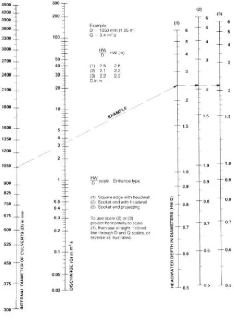
The flow through a culvert is complex and is the result of various parameters. Ideally there are two types of culvert flow control that occur, inlet flow control and outlet flow control. Inlet control occurs when the culvert flow is restricted by the discharge that can pass the inlet for a given headwater (CPAA, p31, 1991). Headwater (HW) is defined as the water level above the invert of the culvert inlet. Outlet control, in contrast, occurs when the culvert flow is restricted by the discharge that can pass the outlet for a given tailwater (CPAA, p31, 1991). Tailwater (TW) is defined as the water level above the invert of the culvert outlet. Figure 1 and Figure 2 illustrate basic examples of inlet control and outlet control.

Figure 1: Culvert Flow Control: Inlet control

HW

Figure 2: Culvert Flow Control: Outlet control

Australian practice for culvert design is based on the hydraulic design manual, “Hydraulic of Precast Conduits” written by CPAA (1991). As stated in the manual,

“it is rarely immediately obvious which pattern of flow a culvert is going to adopt, it is therefore necessary to investigate the consequences of both inlet and outlet control flow.”

(CPAA, p31, 1991)

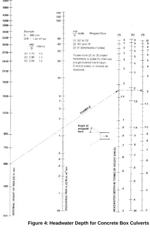
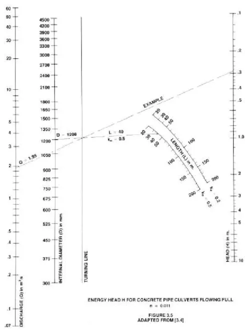
Accessing whether a culvert is flowing under inlet or outlet control requires the use of culvert nomographs produced by the Concrete Pipe Association of Australasia. The nomographs have been produced as a result of various empirical studies and provide an estimation of headwater depth during culvert analysis.

Figure 3: Headwater Depth for Concrete Pipe Culverts with Inlet Control

Figure 4: Headwater Depth for Concrete Box Culverts with Inlet Control

Figure 5: Energy Head H for Concrete Pipe Culverts Flowing Full

Figure 6: Energy Head H for Concrete Box Culverts Flowing Full

Using the nomographs, headwater depths are calculated for the design culvert assuming inlet and outlet control. For inlet control the headwater depth is taken straight from the nomograph. For outlet control, however, the energy head (H) is calculated using the outlet control nomograph, then Equation 1 is used to calculate the headwater depth.

Equation 1:

H

=

HW

+

Ls

−

TW

Where: H = energy head (m)

HW = headwater depth (m)

L = culvert length (m)

s0 = culvert gradient (m/m)

TW = tailwater depth (m)

For outlet control it has been found that if,

Equation 2:

2

D

d

TW

>

+

Where: dc =critical depth (m)

TW = tailwater depth (m)

D = culvert diameter (m)

It has been found that a good approximation of headwater level can be found by using the culvert

nomographs, substituting

2

D

d

+

for TW (CPAA, p37, 1991).

Taking all of these practices into consideration, theory states, whichever control situation produces the greater headwater depth is accepted as the governing culvert control (CPAA, p37, 1991; Chanson, p382, 1999).

Throughout the documentation presented by CPAA there are no statements outlining the assumptions made during the creation of the culvert nomographs. As such the limitations of the methodology produced cannot be deduced. Headwater calculation comparisons using a computer model created by Vienot (2004), based on empirical formulas produced by Chanson (1999), showed however, that the accuracy of the culvert nomograph method was within approximately 5%.

Since it is Australian engineering practice to use the nomograph method, it will be used for the culvert calculations during the study.

3.3.3 Weir Flow

Although there are many types of weir, in the context of this project, the only weirs being researched are broad crested weirs. During flood events it is often the case that structures, such as road and rail embankments or even levy banks, act as broad crested weirs. Figure 7 shows a typical schematic representation of a broad crested weir.

Figure 7: Weir flow

Numerous laboratory-based studies have identified that there are two basic flow regimes that determine the headwater upstream from a broad crested weir. These regimes are known as non-submerged flow and non-submerged flow (Hager & Schwalt, p20, 1994). Non-non-submerged flow is defined to occur when the weir inundation ratio is less than 0.75 Mathematically this is described in Equation 3. Submerged flow therefore occurs for weir flow with an inundation ratio greater than 0.75.

Non-submerged Flow

Non-submerged flow is defined to occur when the weir inundation ratio is less than 0.75 Mathematically this is described in Equation 3.

Equation 3: 0.75 ) ( ) ( 1 2 < − − z d z d

Where: d2 = downstream water depth (m)

d1 = upstream water depth (m)

z = weir height (m)

For non-submerged flow it can be assumed that critical flow conditions occur on the crest of the broad crested weir (Finnemore and Franzini, p534, 2002). Theoretically, flow at critical depth is

Energy Line E1 d1 dc z w d2 Q

dominated by critical flow. This assumption is based on the theory that for non-submerged flow, free overfall flow conditions occur and headwater depth is dependent solely on upstream conditions.

When calculating the upstream depth during non-submerged flow, minimum specific energy calculations are used.

By definition the depth corresponding to the minium specific energy for a given flow is called the specific depth, and for a rectangular channel is given by Equation 4.

Equation 4: 3 1 2      = g q dc

Where: dc = critical depth (m)

q = discharge per unit width (m3/s/m)

g = gravity (m/s2)

Using the calculated critical depth, the minimum specific energy (Emin)for the flow can be calculated

using Equation 5.

Equation 5:

E

d

2

3

min

=

Where: Emin = minimum specific energy (m)

dc = critical depth (m)

Using the Minimum Specific Energy, the upstream specific energy can be calculated using Equation 6.

Equation 6: E₁= z+E_min

Where E1 =upstream specific energy (m)

Emin = minimum specific energy (m)

z = height of weir (m)

Using the calculated upstream specific energy the upstream headwater depth is found using the iterative approach given by Equation 7.

Equation 7: 2 1 2 1 1

2

gd

q

E

d

=

−

Where d1 = upstream depth (m)

E1 = upstream specific energy (m)

q = discharge per unit width (m3/s/m)

g = gravity (m/s2)

Submerged Flow

Submerged flow is defined to occur when the weir inundation ratio is greater than 0.75. During submerged flow, because free overfall flow does not occur, it cannot be assumed that critical flow conditions occur over the broad crested weir. Therefore the headwater depth is dependent on both upstream and downstream conditions. Empirical studies conducted by Bradley (1978), published by the US Department of Transport, have produced calibrated graphs that can be used for discharge coefficient estimation. Figure 9 to Figure 11 show the discharge coefficient graphs and Figure 8 defines the variables used by Bradely (1978).

Figure 8: Weir Flow (Bradley, 1978)

Energy Line

H

Figure 9: Discharge Coefficient Cf (H/L>0.15)

Figure 10: Discharge coefficient Cf (H/L<0.15)

1.66 1.67 1.68 1.69 1.7 1.71 0.14 0.16 0.18 0.2 0.22 0.24 0.26 0.28 0.3 H/L Cf 0 0.2 0.4 0.6 0.8 1 0 0.1 0.2 0.3 0.4 0.5 0.6 0.7 0.8 H(m) Cf

Figure 11: Discharge coefficient Cs (D/H>0.70)

As Defined by Bradley (1978), Equation 8 is used to calculate the upstream water depth H.

Equation 8: 3 2









=

CsCfW

Q

H

Where: H = Upstream water depth (m)

Q = Upstream discharge (m3s-1)

Cs = Discharge coefficient

Cf = Discharge coeffecient

W = Weir Width (m)

Throughout the documentation presented by the Bradley (1978) there are no comments identifying the assumptions or test methodology made during the creation of the submerged weir graphs. As such the limitations of the methodology cannot be estimated. Other contemporary sources of literature, however, such as “Waterway Design – A Guide to the Hydraulic design of Bridges, Culvert and

0.3 0.4 0.5 0.6 0.7 0.8 0.9 1 76 78 80 82 84 86 88 90 92 94 96 98 100 Inundation Ratio Reduction Factor Cs

Floodways” (AUSTROADS, p17 1994), endorse the theory produced by Bradley. AUSTROADS represents the Roads and Traffic Authorities for New South Wales, Queensland, South Australia, Australia Capital Territory and Victoria. As both the Australian and American Road and Traffic Authorities endorse the theory presented by Bradely (1978) it will also be used during this study.

3.3.4 Open Channel Flow

Open channel flow is characterised by a waterway, canal or conduit in which a fluid flows with a free surface, subjected to only by atmospheric pressure (Chanson, p6, 1999; Henderson, p105, 1966).

Open channel Flow can be classified or described in various ways. One classification method is based on the description of the flow, the flow is defined as being either uniform or non uniform.

Steady or uniform flow is defined to occur when the depth of flow within a channel is constant for a given time interval. Unsteady or non-uniform flow, in contrast, is characteristic of flow that changes in depth during a specified time interval.

There have been many studies based on uniform flow and as a result many uniform flow formulas are available. The Kuttat, Bazin, Powell, Chezy and Manning formulas are examples of these. Overall, the empirical formulas are based on the momentum equation, which states the exact balance between the shear forces and the gravity component along a streamline (Chanson, p79, 1999).

Of the uniform flow formulas, the Manning’s formula is the most widely used because of its simplicity and accuracy (Finnemore & Franzini, p412, 2002). The Manning’s formula is shown as

Equation 9:

R

S

A

n

Q

1

=

Where: n = Manning’s n roughness coeffecient

R = Hydraulic Radius (m)

S = Bed Slope (m/m)

A = Cross sectional area

Analysis of the derivation of the Manning’s formula has shown that as an empirical equation, it does not provide exact solutions, however, it can be used as an accurate estimation of normal depth. During the derivation of the formula, the exponent of the hydraulic radius R was based on experimental data taken from artificial channels. For different shapes and roughness, the average value of the exponent was found to vary from 0.6499 to 0.8395. Using these values the approximate value of 2/3 was adopted for the exponent (Chow, p99, 1959).

Authors such as Finnemore & Franzini (2002), Chow (1959) and Hamill (1995) recommend the use of Manning’s formula instead other uniform flow formulas. Manning’s formula was used for the open channel calculations throughout this study.

4

M

ETHODOLOGY

4.1 General

When discussing environmental models, it is recognised that the effectiveness of numerical models, such as TUFLOW, are dependent on three main factors. These are

• the quality of physical data used during model development,

• the competence of the modeller to produce a model that is representative of the natural system and

• the numerical capability of the model to replicate certain aspects of a given system (Barton, p1, 2001)

To minimise the possibility of physical data affecting test results, hypothetical models were created and used for all the testing. The use of hydraulic theory was used instead of real data to estimate expected flow conditions for the given model case during the testing. This testing structure was favoured for a variety of reasons. These were,

1. Elimination of possible inaccuracies in physical data.

2. The possibility for the testing of model features against an infinite number of test conditions. During the initial scoping of the project it was realised that relying on actual physical data may limit the possibility to test all flow regimes and variables.

The testing was structured so that the “test model” results were compared against independent calculations based on established engineering principles. The comparison results will be calculated in absolute terms and relative terms. The absolute variation shows the depth variation of the results in metres, the relative variation, meanwhile, can be defined as the calculated depth variation as a percent difference. The use of independent calculations based on engineering principles ensures the numerical capabilities of the solution scheme utilized by the TUFLOW program is solely tested in an organised manner.

Whilst planning the model testing, establishing the testing structure for each hydraulic feature required the consideration of two main factors. These factors were related to the modelling structure of TUFLOW, and the hydraulic principles describing the fluid flow.

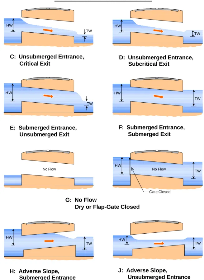
Initially the modelling structure utilised by TUFLOW was considered. This ensured that each regime used by the particular feature was tested. During culvert flow, for example, the modelling structure of

TUFLOW splits the culvert flow into 12 separate flow regimes (A-J) depending on variables such as bed slope, inlet submergence and outlet submergence.

Secondly the engineering theory used to represent the hydraulic flow was analysed. This ensured that each flow regime and variable with relevance to the engineering theory for the hydraulic feature was also tested. For example, open channel flow testing was conducted for supercritical, critical and subcritical flow regimes. During each regime test, the variables of channel width, bed slope and Manning’s roughness coefficient were also tested.

This testing structure has been used such that the testing of TUFLOW has been carried out in a concise, structured format.

4.2 Model Structure

Developing a TUFLOW model, representative of a given system, requires a variety of different data sets. These data sets define the transport of fluid within the model and the fluid volume entering and leaving the model. Factors affecting fluid transport are obtained in the form of GIS layers defining digital terrain models, hydraulic structure geometry and Manning’s roughness coefficients. Fluid volumes entering and leaving the model extents are described as boundary conditions.

4.2.1 Fluid Transport

4.2.1.1 Digital Terrain Model

A Digital Terrain Model (DTM) is a topographic map used to define all flow paths and storage areas within the 2D domain. It is recommended that the vertical accuracy of larger models be within 0.2m, whilst for fine scale urban models 0.1m is recommended (WBM Oceanics Australia, p38, 2004).

4.2.1.2 Hydraulic Structures

The geometry of all hydraulic structures must be defined. This requires accurate cross section data which can often be obtained from structural plans or may need to be obtained by onsite observation and surveying.

To minimise the possibility of erroneous results during the project caused by DTM and cross section inaccuracies, hypothetical models have been used for the testing.

4.2.1.3 Manning’s Roughness Coefficient

Bed resistance values are defined for areas defined within the bounds of the DTM by an assigned Manning’s n value.

During the testing, hypothetical models will be used, such that the full range of Manning’s n values can be tested, whilst reducing possible inaccuracies of using “real” data.

4.2.2 Boundary Conditions

Boundary conditions define the amount of fluid entering and exiting the model.

All upstream boundary conditions were assigned a QT flag, defining the boundary condition to be set in a flow vs time format. All downstream boundary conditions were assigned a HT flag, defining the format of the boundary condition to be, head vs time.

4.3 Model Run

Conventionally there are two types of model run which can be modelled, static and dynamic. A static run is characterised by fixed boundary conditions, simulating uniform flow conditions. In contrast, a dynamic run commonly has boundary conditions which change over time, characteristic of non-uniform flow.

During the testing, static runs were used to test the accuracy of the modelling program against independent calculations. Dynamic runs, on the other hand, were used to test the transition of flow between regimes. For example, culvert flow dynamic runs were used to test the transition between flow governed by inlet and outlet control.

5

I

NDEPENDENT

T

ESTING

5.1 Culvert Analysis

A culvert is a covered channel designed to pass water through an embankment, such as under a highway, railroad or through a dam (Chanson, p365, 1999). A culvert consists of three sections, the inlet, the throat and the outlet. In cross section a culvert may be circular (pipe culvert) or rectangular (box culvert) in shape. In practice a culvert is designed to pass a specific flow rate with an associated natural flood level. Its hydraulic performances are the design discharge, the upstream depth and the maximum acceptable head loss. The hydraulic design of a culvert is basically the selection of an optimum compromise between discharge capacity and head loss (Chanson, p369, 1999).

Culvert flow is one directional in nature. In order to obtain a better representation of the hydraulic scenario and for computational efficiency TUFLOW utilises the 1D-modelling program, ESTRY, for culvert analysis. ESTRY uses various culvert regimes, based on flow characteristics, to represent culvert flow. Figure 12 and Figure 13 illustrate the culvert classifications used by ESTRY.

TW

A: Unsubmerged Entrance, Supercritical Slope

B: Submerged Entrance, Supercritical Slope INLET CONTROL FLOW REGIMES

HW TW HW TW K: Unsubmerged Entrance, Submerged Exit Critical at Entrance L: Submerged Entrance, Submerged Exit

Orifice Flow at Entrance

HW

TW

HW

Figure 12: ID inlet Control Culvert Flow Regimes

C: Unsubmerged Entrance,

Critical Exit

D: Unsubmerged Entrance,

Subcritical Exit

E: Submerged Entrance,

Unsubmerged Exit

G: No Flow

Dry or Flap-Gate Closed

F: Submerged Entrance,

Submerged Exit

OUTLET CONTROL FLOW REGIMES

HW TW HW TW HW TW No Flow HW TW HW TW

H: Adverse Slope,

Submerged Entrance

J: Adverse Slope,

Unsubmerged Entrance

(Critical or Subcritical at Exit)

HW

TW No Flow

Gate Closed

Figure 13: 1D Outlet Control Culvert Flow Regimes (WBM, p44-45, 2004)

5.1.1 Computational Procedure

The computational procedure used to test culvert flows consisted of three tests. Initially each culvert regime (A-K), as defined by ESTRY, was tested; secondly, culvert parameters were tested. The parameters tested were;

• Culvert length

• Culvert width

• Entry loss coefficients

• Culvert number

Finally, non-uniform flow tests were used to check the ability of ESTRY to model the transition of flow between different flow regimes, based on engineering theory. This ensures the transition between inlet and outlet controlled flow is tested.

These tests were undertaken for pipe and rectangular culverts. A summary of the simulations undertaken is provided in Table 2 and Table 3.

Table 2: Summary of Pipe Culvert Simulation – Regime test Run Flow Regime Inflow (ms-1) Downstream Depth (m) Diameter (mm) Length (m) Entry Loss (ke) Upstream invert (m) Downstream invert (m) Number of culverts 1 A 2 7.1 1500 35 0.5 7.5 7 1 2 B 6.5 8.1 1500 35 0.5 10 7 1 3 C 2 6.5 1500 35 0.5 7 7 1 4 D 0.5 8 1500 35 0.5 7 7.5 1 5 E 5 6.5 1500 35 0.5 7 7 1 6 F 8 9.2 1500 35 0.5 8 7 1 7 H 5 7.7 1500 35 0.5 6.5 7 1 8 J 2 7.7 1500 35 0.5 6.5 7 1 9 K 10 L 6.5 8.5 1500 35 0.5 10 7 1

Table 3: Summary of Pipe Culvert Simulations - Variable Test Run Inflow (ms-1) Downstream Depth (m) Diameter (mm) Length (m) Entry loss (ke) Number of culverts Upstream invert (m) Downstream invert (m) Tailwater depth (m) 11 3.5 7.4 1500 35 0.5 1 7 6.5 0.4 12 3.5 7.4 1500 50 0.5 1 7 6.5 0.4 13 3.5 7.4 1500 20 0.5 1 7 6.5 0.4 14 3.5 7.4 1500 35 0.2 1 7 6.5 0.4 15 3.5 7.4 1500 35 0.8 1 7 6.5 0.4 16 3.5 7.4 900 35 0.5 1 7 6.5 0.4 17 3.5 7.4 2100 35 0.5 1 7 6.5 0.4 18 3.5 7.4 1500 35 0.5 2 7 6.5 0.4 19 3.5 7.4 1500 50 0.5 1 7 6.5 2.0 20 3.5 7.4 1500 20 0.5 1 7 6.5 2.0

Table 4: Summary of Rectangular Culvert Simulations - Regime Test Run Flow Regime Inflow (m3s-1) Downstream Depth (m) Height (mm) Diameter (mm) Length (m) Entry Loss (ke) Upstream invert (m) Downstream invert (m) Number of culverts 21 A 3.5 7.1 1500 1500 35 0.5 7.5 7 1 22 B 6.5 8.1 1500 1500 35 0.5 10 7 1 23 C 2 7.1 1500 1500 35 0.5 7 7 1 24 D 0.5 8 1500 1500 35 0.5 7 7 1 25 E 5 6.5 1500 1500 35 0.5 7 7 1 26 F 8 9.2 1500 1500 35 0.5 8 7 1 27 H 5 7.7 1500 1500 35 0.5 6.5 7 1 28 J 0.5 7.1 1500 1500 35 0.5 6 7 1 29 K 5.8 8.9 1500 1500 35 0.5 10 7 1 30 L 6.5 8.5 1500 1500 35 0.5 10 7 1

Table 5: Summary of Rectangular Culvert Simulations - Variable Test Run Inflow (m3s-1) Downstrea m Depth (m) Height (mm) Width (mm) Length (m) Entry Loss (ke) Number of culverts Upstream invert (m) Downstream invert (m) Tailwater depth (m) 31 3.5 7.4 1500 1500 35 0.5 1 7 6.5 0.4 32 3.5 7.4 1500 1500 50 0.5 1 7 6.5 0.4 33 3.5 7.4 1500 1500 20 0.5 1 7 6.5 0.4 34 3.5 7.4 1500 1500 35 0.2 1 7 6.5 0.4 35 3.5 7.4 1500 1500 35 0.8 1 7 6.5 0.4 36 3.5 7.4 1500 900 35 0.5 1 7 6.5 0.4 37 3.5 7.4 1500 2100 35 0.5 1 7 6.5 0.4 38 3.5 7.4 1500 1500 35 0.5 2 7 6.5 0.4 39 3.5 7.4 1500 1500 50 0.5 1 7 6.5 2 40 3.5 7.4 1500 1500 20 0.5 1 7 6.5 2

For non-uniform testing, a pipe culvert of 1.5m diameter and a rectangular culvert of the dimensions 1.5m x 1.5m was used. The following variables were assigned to the test culverts.

• Entry loss = 0.5

• Exit loss = 1.0

• Height contraction coefficient = 0.8

• Width contraction coefficients = 1.0

• Length = 35m

• Number of culverts =1

Table 6: Culvert Flow - Non-uniform flow conditions

Run Time (hours) Inflow (m3s-1) Downstream Depth (m)

0 1.5 7.5 1 1.5 7.5 2 1.5 8 3 1.5 9 4 1.5 9.5 5 1.5 9 6 1.5 8 41 (pipe culvert), 42 (Rectangular culvert) 7 1.5 7.5

5.1.2 Results

5.1.2.1 Uniform Flow

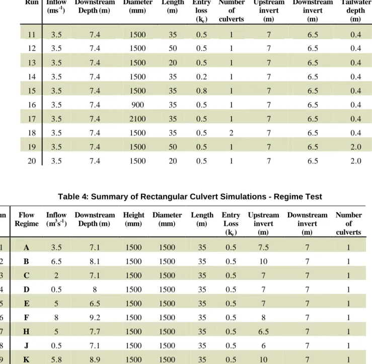
A summary of the culvert test results is given graphically Figure 14 to Figure 17.

Runs 1-10 were used to test that ESTRY was representing each culvert regime (as defined by

ESTRY) accurately for pipe culverts. The test results are shown in Figure 14.

Figure 14: Pipe Culvert - Regime Results

0.00 2.00 4.00 6.00 8.00 10.00 12.00 14.00 A B C D E F H J K L ESTRY Regime Headwater Depth (m) 0.00% 1.50% 3.00% 4.50% 6.00% 7.50% 9.00% 10.50% 12.00% 13.50% 15.00% Variation Independent Calculations ESTRY output Variation Nomograph accuracy

Runs 11-20 tested the variables that contribute to headwater depth calculations for circular culverts. Listed below are the variables tested for each run.

• Run 11 - base run to which all other runs could be compared against

• Run 12 and 13 - culvert length during inlet control

• Run 14 and 15 - culvert entrance losses

• Run 16 and 17 – culvert diameter

• Run 18 – number of culverts

• Run 19 and 20 – culvert length during outlet control conditions

Figure 15: Pipe Culvert – Variable Results

0.00 2.00 4.00 6.00 8.00 10.00 12.00 14.00

Base case (Run 11)

length =50m (ic) (Run 12)_{length = 20m (ic) (Run 13)}

ke =0.2 (Run 14)ke= 0.8 (Run 15)

Dia = 900mm (Run 16)_{Dia =2100mm (Run 17)no culverts =2 (Run 18)}

length =50m (oc) (Run 19)length =20 (oc) (Run 20)

Variable test Headwater Depth (m) 0.00% 1.50% 3.00% 4.50% 6.00% 7.50% 9.00% 10.50% 12.00% 13.50% 15.00% Variation Independent Calculations ESTRY output Variation Nomograph accuracy

Runs 21-30 were used to test that ESTRY was representing each culvert regime accurately for box culverts. The test results are shown in Figure 16

Figure 16: Box Culvert - Regime Results

0.00 2.00 4.00 6.00 8.00 10.00 12.00 14.00 A B C D E F H J K L ESTRY Regime Headwater Depth (m) 0.00% 1.50% 3.00% 4.50% 6.00% 7.50% 9.00% 10.50% 12.00% 13.50% 15.00% Variation Independent Calculations ESTRY output Variation Nomograph accuracy

Runs 31-40 tested the variables that contribute to headwater depth calculations for box culverts. Listed below are the test explanations for each run.

• Run 31 - base run to which all other runs could be compared against

• Run 32 and 33 - culvert length during inlet control

• Run 34 and 35 - culvert entrance losses

• Run 36 and 37 – culvert width

• Run 38 – number of culverts

• Run 39 and 40 – culvert length during outlet control

Figure 17: Box Culvert – Variable Results

8.20 8.40 8.60 8.80 9.00 9.20 9.40 9.60 9.80 10.00

Base case (Run 31)

length =50m (ic) (Run 32)_{length = 20m (ic) (Run 33)}

ke =0.2 (Run 34)ke= 0.8 (Run 35)

Width = 900mm (Run 36)Width =2100mm (Run 37)no culverts =2 (Run 38)length =50m (oc) (Run 39)length =20 (oc) (Run 40)

Variable test Headwater Depth (m) 0.00% 1.50% 3.00% 4.50% 6.00% 7.50% 9.00% 10.50% 12.00% 13.50% 15.00% Variation Independent Calculations ESTRY output Variation Nomograph accuracy

5.1.2.2 Non-Uniform flow

Run 41 and 42 tests the transition of flow from inlet to outlet control, and vice versa. The testing has been conducted on pipe and box culverts.

Figure 18: Pipe Culvert - Non Uniform Flow Results

Figure 19: Box Culvert - Non Uniform Flow Results

6 6.5 7 7.5 8 8.5 9 9.5 10 0:00 1:00 2:00 3:00 4:00 5:00 6:00 7:00 8:00 Time (hours) Headwater Depth (m) 0% 1% 2% 3% 4% 5% 6% 7% 8% 9% 10% ESTRY Output Independent Calculations Downstream depth Variation Flow Regime

Outlet Control Inlet Control Inlet Control 6 6.5 7 7.5 8 8.5 9 9.5 10 0:00 1:00 2:00 3:00 4:00 5:00 6:00 7:00 8:00 Time (hours) Headwater Depth (m) 0% 1% 2% 3% 4% 5% 6% 7% 8% 9% 10% ESTRYOutput Independent Calculations Downstream Depth Variation Flow Regime

Outlet Control Inlet Control Inlet Control

5.1.3 Discussion

The culvert testing initially tested the culvert regimes identified by the ESTRY program. Secondly, variables affecting headwater depth based on engineering theory were tested. During the testing of the variables it was considered important to test culvert flow under inlet and outlet control. Finally the transition of flow between inlet and outlet control was tested.

During inlet control, theory states that conditions downstream of the culvert inlet do not contribute to the headwater depth. This means that entry losses and culvert diameter are the dominant variables contributing to headwater depth. Culvert length, however, has no effect on headwater depth. The results show that ESTRY represents inlet control correctly.

Under outlet control downstream conditions influence headwater depth. In contrast to inlet controlled flow conditions, culvert length affects headwater depth. When experiencing outlet control the results show that ESTRY operates correctly, and as expected, the culvert length influences the headwater depth.

The steady state model runs testing inlet and outlet controlled flow regimes indicate that ESTRY provides accurate estimations for headwater depth. To complete the culvert analysis it was considered necessary to also assess the capabilities of ESTRY to estimate flow that is experiencing a flow regime change. Dynamic models were created, modelling a test culvert that was flowing initially under inlet control. The flow was varied such that the culvert flow developed into outlet-controlled flow, after a period of time, the culvert flow was then returned to inlet control. The testing indicated that ESTRY effectively models the transition of flow between inlet and outlet control, for both, pipe and rectangular culverts.

Overall, the results show that ESTRY produces results similar to predicted headwater depths using the culvert nomograph method developed by the CPAA (1991). The variation in the results ranged from 0.11% to 5%, equalling a maximum flow depth variation of 0.4m. The average variation of the results was calculated to be 1.69%, which in absolute terms, is an average depth variation of 0.14m.

During the study it was expected that the ESTRY output would vary from the calculated depth by up to 5%. This was assumed based on the creation of the culvert nomographs used for the testing. The nomographs were produced from empirical laboratory studies and it is recognised that they are only a method of headwater depth estimation.

Since the ESTRY results all produce values with a variation less than 5%, the testing shows that ESTRY is representing culvert flow consistent with current engineering depth estimation practices.

5.2 Weir Flow

A weir is an obstruction in a channel that raises the upstream water level, whilst allowing fluid flow to pass over or through the obstruction (Streeter, p416, 1958). In practice, a weir is an accurate flow-measuring device (Chow, p360, 1973). As such they are often designed for that purpose.

Although there are many types of weirs, in the context of this project, the only weirs being researched are broad crested weirs. During flood events it is often the case that structures, such as road and rail embankments or even levee banks, act as broad crested weirs. Other weir types such as the Sharp Crested weir and the Ogee weir vary rarely occur in the natural or urbanised environments unless they were designed for a specific purpose, such as for flow measurement. Figure 3 shows a section of a broad crested weir.

Figure 20: Broad Crested Weir

A broad crested weir is a flat-crested structure with a flow length (L), represented by the distance across the flow path at the weir crest, large compared with the flow thickness. The ratio of flow length of the weir to upstream head over crest must typically be greater than 1.5 to 3 (Chow, p410, 1973).

Research has found there are typically two types of flow encountered during weir flow; these are described as submerged and non-submerged flow.

5.2.1 Computational Procedure

TUFLOW has been designed such that a weir can be represented either as a 1D or 2D structure. Basically, the size of the weir structure relative to the chosen grid size of the 2D domain defines whether the weir is better suited to 1D or 2D modelling. Ideally, this means that weirs of small flow length are often represented in 1D and weirs of greater flow length are modelled in 2D. During the testing, both 1D and 2D structures were analysed for flow conditions which were:

Energy Line E1 d1 dc z W d2 Q

• Non-submerged

• Submerged

• Transitional (Moving from submerged into non-submerged flow conditions).

The non-submerged and submerged flow was tested using steady state flow conditions. The transitional testing was conducted using non-uniform flow.

5.2.1.1 1D Weir Flow

Non-submerged flow was tested varying; upstream discharge, downstream depth and the flow length were varied. During the testing a weir with a height of 5 metres was used.

Table 7 shows the variables that were tested for free overfall flow conditions.

Table 7: 1D Non-submerged Flow

Run Upstream Discharge, Q

(m3s-1) Downstream Depth, d2 (m) Flow Length, L (m) 1 1 4 5 2 3 4 5 3 5 4 5 4 7 4 5 5 1 4.5 5 6 3 4.5 5 7 5 4.5 5 8 7 4.5 5 9 1 5 5 10 3 5 5 11 5 5 5 12 7 5 5 13 1 4.99 5 14 3 4.99 5 15 5 4.99 5 16 7 4.99 5 17 1 4.99 10 18 3 4.99 10 19 5 4.99 10 20 7 4.99 10 21 1 4.99 20

22 3 4.99 20

23 5 4.99 20

24 7 4.99 20

During submerged flow testing; upstream discharge and the weir width were varied. The downstream depth was maintained constant, at 5.5 metres, to ensure that the flow conditions remained as submerged flow. Table 8 shows the variables that were tested for submerged flow conditions.

Table 8: 1D Submerged Flow

Run Upstream Discharge Q

(m3s-1) Downstream Depth d2 (m) Flow Length, L (m) 25 1 5.5 5 26 3 5.5 5 27 5 5.5 5 28 7 5.5 5 29 1 5.5 10 30 3 5.5 10 31 5 5.5 10 32 7 5.5 10 33 1 5.5 20 34 3 5.5 20 35 5 5.5 20 36 7 5.5 20

The transition of flow from submerged to non-submerged flow was tested using a dynamic model, under non-uniform flow conditions. A flow length of 5 metres and a downstream depth of 5.5 metres were used for the testing. The upstream discharge was increased from 1m3s-1 to 16 m3s-1; this ensured that the weir was initially flowing under submerged flow before developing into non-submerged flow. Table 9 shows the variables that were used for transitional flow testing.

Table 9: 1D Flow Transition Test

Run Upstream Discharge,

Q (m3s-1) Time, t (hours) Downstream Depth, d2 (m) Flow Length, L (m) 37 1 0 5.5 5 1.5 1 5.5 5 2 2 5.5 5 2.5 3 5.5 5 3 4 5.5 5 3.5 5 5.5 5 4 6 5.5 5 4.5 7 5.5 5 5 8 5.5 5 5.5 9 5.5 5 6 10 5.5 5 6.5 11 5.5 5 7 12 5.5 5 16 13 5.5 5

5.2.1.2 2D Weir Flow

During the testing a weir with a height of 5 metres was used.

Non-submerged flow was tested varying the; upstream discharge, downstream depth and the flow length. Table 10 shows the variables that were tested.

Table 10: 2D Non-submerged Flow

Run Upstream Discharge Q

(m3s-1) Downstream Depth d2 (m) Flow Length, L (m) 1 10 4 20 2 15 4 20 3 20 4 20 4 10 4.5 20 5 15 4.5 20 6 20 4.5 20 7 10 5 20 8 15 5 20 9 20 5 20 10 10 5 30 11 15 5 30 12 20 5 30 13 10 5 40 14 15 5 40 15 20 5 40

During submerged flow testing; upstream discharge and the weir width were varied. The downstream depth was maintained constant, at 5.5 metres, to ensure that the flow conditions remained as submerged flow. Table 11 shows the variables that were tested for submerged flow conditions.

Table 11: 2D Submerged Flow

Run Upstream Discharge, Q

(m3s-1) Downstream Depth, d2 (m) Flow Length, L (m) 16 10 5.5 20 17 15 5.5 20 18 20 5.5 20 19 10 5.5 30 20 15 5.5 30 21 20 5.5 30 22 10 5.5 40 23 15 5.5 40 24 20 5.5 40

The transition of flow from submerged to non-submerged flow was tested using a dynamic model. The model used a flow length of 20 metres and a constant downstream depth of 5.5 metres. The upstream discharge was increased from 10m3s-1 to 40 m3s-1. The change in upstream discharge, with constant downstream depth ensured that the weir was initially flowing under submerged flow before developing into non-submerged flow. Table 12 shows the variables that were used for transitional flow testing.

Table 12: 2D Flow Transition Test

Run Upstream Discharge,

Q (m3s-1) Time, t (hours) Downstream Depth, d2(m) Flow Length, L (m) 25 10 0 5.5 20 11 1 5.5 20 12 2 5.5 20 13 3 5.5 20 14 4 5.5 20 15 5 5.5 20 16 6 5.5 20 17 7 5.5 20 18 8 5.5 20 19 9 5.5 20 20 10 5.5 20 40 11 5.5 20

5.2.2 Results

5.2.2.1 ID Weir Results

A summary of the 1D weir test results is given in Figure 21 to Figure 24.

Runs 1-12 were used to test that ESTRY was representing non-submerged flow accurately. During non-submerged flow, because of free overfall conditions, the downstream depth has no influence on the upstream depth. As expected all runs with identical upstream discharges produced identical upstream depth estimations, independent of downstream depth. The model runs that were found to have identical results are listed;

• Runs 1,5,9

• Runs 2,6,10

• Runs 3,7,11

• Runs 4,8,12.

The results can be seen in Table 13 this has also been graphically shown in Figure 21.

Table 13: 1D Non-submerged Flow – Results (Downstream Depth)

Run Upstream Depth

Independent Calculation (m) Upstream Depth ESTRY Output (m) Variation (%) 1,5,9 5.24 5.24 0.04% 2,6,10 5.50 5.50 0.09% 3,7,11 5.70 5.71 0.13% 4,8,12 5.87 5.89 0.18%

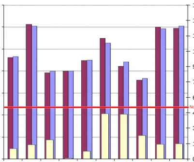
Figure 21: 1D Non-submerged Flow – Results (Downstream Depth) 5 5.2 5.4 5.6 5.8 6 0 1 2 3 4 5 6 7 8 Upstream Discharge Q (m3s-1) Upstream Depth d1 (m) 0.00% 1.00% 2.00% 3.00% 4.00% 5.00% 6.00% 7.00% 8.00% 9.00% 10.00% Variation Run 1-12 independent calculations Run 1-12 ESTRY output Variation

Runs 13-24 were used to test that ESTRY was representing non-submerged flow accurately for varying weir widths. Since upstream conditions influence downstream depth during non-submerged flow it was expected that for wider weir widths, as defined by the continuity equation, lower upstream depths would be produced. The results are presented in Figure 22.

Figure 22: 1D Non-submerged Flow – Results (Flow Length)

5.00 5.20 5.40 5.60 5.80 6.00 0 1 2 3 4 5 6 7 8 Upstream Discharge Q (m3s- 1) Upstream Depth d 1 (m) 0.00% 1.00% 2.00% 3.00% 4.00% 5.00% 6.00% 7.00% 8.00% 9.00% 10.00% Variation L=5m independent calculations L=5m ESTRY output L=10m independent calculations L=10m ESTRY output L=20m independent calculations L=20m ESTRY output L=5m Variation L=10m Variation L=20m Variation

Runs 25-36 were used to test that ESTRY was representing submerged flow accurately for varying weir flow lengths. Since both upstream and downstream conditions influence upstream depth during submerged flow it was expected that for greater flow lengths, with a constant downstream level, lower upstream depths would be produced. The results are presented in Figure 23.

In addition to submerged flow it was also tested that ESTRY could function for flow conditions which where conventionally in the reverse direction. To achieve this, the upstream discharge used was designed to be small enough in magnitude to provide an upstream head less than the downstream depth. The conservation of momentum defines that water flows from a greater elevation to a lower elevation due to gravitational forces. Conventionally this means that flow is expected to move from downstream, upstream, in the reverse direction. For varying discharges this was tested for all flow lengths and can be seen when the upstream depth is equal to the downstream depth, 5.5m. The results are presented in Figure 23.

Figure 23: 1D Submerged Flow - Results

5.00 5.20 5.40 5.60 5.80 6.00 0 1 2 3 4 5 6 7 8 Upstream Discharge Q (m3s-1) Upstream Depth d1 (m) 0.00% 1.00% 2.00% 3.00% 4.00% 5.00% 6.00% 7.00% 8.00% 9.00% 10.00% Variation L=5m independent calculations L=5m ESTRY output L=10m independent calculations L=10m ESTRY output L=20m independent calculations L=20m ESTRY output L=5m Variation L=10m Variation L=20m Variation