THREE ESSAYS ON DEVELOPMENT AND LABOR
ECONOMICS
A Dissertation
Presented to the Faculty of the Graduate School of Cornell University
in Partial Fulfillment of the Requirements for the Degree of Doctor of Philosophy
by Yanan Li May 2018
c
2018 Yanan Li ALL RIGHTS RESERVED
THREE ESSAYS ON DEVELOPMENT AND LABOR ECONOMICS Yanan Li, Ph.D.
Cornell University 2018
My dissertation comprises three empirical studies on development and labor economics. The first two essays are in the context of National Employment Guarantee Schemes (thereafter, NREGA) in India. In the first one, I study whether existing inequality hinders the implementations of NREGA, using district-level data on land ownership distribution and the implementations of NREGA. To address potential endogeneity issues, I leverage a historical institu-tion in India, the land revenue collecinstitu-tion system established by British colonial rulers during 1750-1861, to construct an instrumental variable for land inequal-ity. Both OLS and instrumental variable results give robust evidence that the concentration of land ownership reduces public works provision. This relation-ship could be explained by the mechanism that public works schemes raise agri-cultural wages in the private labor market, thereby incentivizing big landlords to use their political power to oppose this program. This paper provides the first empirical evidence that the concentration of landownership, a proxy for political power, is a hurdle to providing public employment to the poor. In the second essay, I focus on the participants of NREGA and study the wage bar-gaining effect of participating in NREGA. Using a household level panel and a difference-in-differences framework, I find indirect evidence that participat-ing in NREGA would increase the wage bargainparticipat-ing power for both participants themselves and for their spouses in the private labor market.
wage standards in China. I utilize a spatial lag methodology to study city-level strategic interactions in setting and enforcing minimum wage standards during 2004-2012 in China. This analysis finds strong evidence of spatial inter-dependence in minimum wage standards and enforcement among main cities in China. If other cities decrease minimum wage standards by 1 RMB, the host city will decrease its standard by about 0.7-3.2 RMB. If the violation rate in other cities increases by 1 percentage point, the host city will respond by an increase of roughly 0.4-1.0 percentage points. These interactions suggest the need for policy coordination in labor regulation.
BIOGRAPHICAL SKETCH
The author of the dissertation, Yanan Li, is a PhD candidate in the Dyson School of Applied Economics and Management at Cornell University. She received a bachelor’s degree in agricultural economics and management from Zhejiang University in 2010 and a master’s degree in agricultural economics from Ren-min University of China in 2012. She will join the economics department in Beijing Normal University in 2018 fall.
ACKNOWLEDGEMENTS
I would like to express the deepest appreciation to my special committee chair, Ravi Kanbur, and to the remaining members of my committee: Christopher Boone, Lawrence Kahn and Victoria Prowse. Thanks to Ravi for many insight-ful conversations and for guiding me through the PhD program. His passion in both research and teaching is always an inspiration. Thanks to Lawrence for always offering brilliant comments and suggestions on my projects. For teach-ing me a variety of empirical techniques, I am grateful to Victoria. Workteach-ing with her has been one of the best experiences of my PhD by far. I am especially grateful to Chris for his constructive suggestions on my job market paper and his support during the job market season. Without the kind help and support of my committee, this dissertation would not have been possible.
During my PhD study, I also greatly benefited from interacting with other professors and researchers both in and outside of Cornell University. Special thanks go to Yanyan Liu and Shanjun Li, who have given me substantial help and support over the years. I am also grateful to Christ Barrett, Arnab Basu, Leah Bevis, Nancy Chau, Ritam Chaurey, John Hoddinott, Mallika Thomas, Xi-aobo Zhang and Laura Zimmermann, who have each kindly offered very help-ful comments on my dissertation.
One of the best things at Cornell is to be surrounded by talented peers. Spe-cial thanks go to Jakina Debnam, Naveen Sunder and Haoying Wang, who have offered extensive discussions on my dissertation and helped me through the hard times. I also want to thank Maulik Jagnani, Vesall Nourani, Tanvi Rao and the attendees from AEM development research seminar.
Winter in Ithaca is usually long. I feel extremely fortunate to have had the best cohort, including Jennifer Denno Ciss´e, Jakina Debnam, Xiaoli Fan, Jie Li
and Linden McBride. I will remember forever those days when we were young and together. I have also received help and support from many others at Cor-nell including Ying Ji, Lisha Liu, Hang L ¨u, Jing Qian, Xiaowen Shi, Vidhya Soundararajan, Yue Wang, Kai Wu, Dafeng Xu, Yi Xu, Linlin Zhang, Yang Zhang and many others.
In addition, I would like to thank Jun Xiong, who is always there to listen and support. I would also like to thank my undergraduate professor Hongdong Guo, for his encouragement throughout the years. And thanks to my coauthor Wangyang Lai for his help in the job market season.
Lastly, I would like to thank my best friend, Wenjun Wang, for always being there. Thanks to my mother and father for giving me this incredible educational opportunity.
May 10, 2018 at Bogot´a, Colombia
CONTENTS
Biographical Sketch . . . iii
Dedication . . . iv
Acknowledgements . . . v
Contents . . . vii
List of Tables . . . ix
List of Figures . . . x
1 Land Inequality and the Provision of Public Works—Evidence from National Rural Employment Guarantee Scheme in India 1 1.1 Abstract . . . 1
1.2 Introduction . . . 2
1.3 Background: The National Rural Employment Guarantee Act . . 8
1.3.1 Demand-Driven Nature of NREGA Employment . . . 8
1.3.2 Financing NREGA and the Supply Constraint . . . 9
1.3.3 Landlords and NREGA Employment . . . 11
1.4 Mechanism . . . 13
1.5 Data . . . 14
1.5.1 Land Inequality . . . 14
1.5.2 NREGA Implementation . . . 16
1.5.3 Demographic and Geographic Information . . . 17
1.6 Empirical Model and Results . . . 21
1.6.1 OLS Results . . . 21
1.6.2 Addressing Endogeneity . . . 23
1.6.3 IV Results . . . 30
1.7 Robustness of the Identification . . . 36
1.7.1 Robustness to Violations of Perfect Exogeneity . . . 36
1.7.2 Alternative Measurements of NREGA Implementations . 39 1.7.3 Does Gini Coefficient Capture the Top Distribution?— Alternative Measurement of Land Inequality . . . 42
1.7.4 Is NREGA Demand Higher in More Equal Areas? . . . 43
1.8 Conclusion . . . 48
2 Does Participating in Public Works Increase Wage Bargaining Power in Private Sectors? — Evidence from National Rural Employment Guarantee Scheme in India 53 2.1 Abstract . . . 53
2.2 Introduction . . . 54
2.3 Program Background . . . 60
2.3.1 Wage and Rationing of NREGA work . . . 60
2.3.2 Seasonality of NREGA works . . . 61
2.4 Modeling and Hypothesis . . . 62
2.5.1 Program roll out and take-up . . . 65
2.5.2 Descriptives . . . 67
2.6 Empirical Model and Identification . . . 70
2.7 Results . . . 73
2.7.1 When husbands work in NREGA . . . 74
2.7.2 When wives work in NREGA . . . 77
2.7.3 Pattern of treatment effects . . . 79
2.8 Conclusion and Discussion . . . 80
3 Minimum Wage Competition between Local Governments in China 87 3.1 Abstract . . . 87
3.2 Introduction . . . 88
3.3 Institutional Background . . . 90
3.3.1 Minimum wage setting and enforcement in China . . . 90
3.3.2 Motivation of local leaders to compete on minimum wages . . . 92
3.4 Data . . . 93
3.5 Empirical Specification . . . 96
3.5.1 Race on minimum wage standards . . . 97
3.5.2 Race on minimum wage enforcement . . . 99
3.6 Main Results . . . 101
3.6.1 Race on minimum wage standards . . . 101
3.6.2 Race on enforcement . . . 102
3.7 Robustness checks . . . 104
3.7.1 Robustness to sample changes . . . 104
3.7.2 Robustness of results to alternative weighting matrices . . 108
3.8 Conclusion . . . 110
A Chapter 2 of Appendix 115
LIST OF TABLES
1.1 Timelines for various steps involved in preparation and finaliza-tion of annual labor budget. . . 11 1.2 Summary statistics of NREGA implementation . . . 12 1.3 Descriptives of land inequality and demographic information . . 20 1.4 Dep var: % of households provided with NREGA jobs (OLS) . . 24 1.5 State-wise distribution of landlord and non-landlord districts . . 26 1.6 Dep var: Land inequality (gini coefficient) in 2005, (First stage) . 31 1.7 Dep var: % of households provided with NREGA jobs . . . 33 1.8 Robustness checks: Alternative measurements of NREGA
im-plementation . . . 41 1.9 Robustness check: Dependent variable—Share of land by top
10% land holdings (First Stage) . . . 45 1.10 Robustness check: land inequality measured as the share of land
by top 10% land holdings . . . 46 1.11 Do districts with more equal land distributions have worse labor
markets? . . . 49 1.12 Robustness of main effects to the control of agricultural wages . 50 2.1 Program phased roll-out at village and individual level . . . 66 2.2 Descriptive statistics – three group comparison . . . 68 2.3 Men’s Self Response, using NREGA payment 300 Rupees as cut
off . . . 75 2.4 Spousal response, wife to husband, NREGA payment 300
Ru-pees above . . . 76 2.5 Women’s Self Response, using NREGA payment 300 Rupees as
cut off . . . 78 2.6 spousal response, Husband to wife, NREGA payment 300
Ru-pees above . . . 79 3.1 Trend of minimum wage standards, 2004-2012 . . . 96 3.2 Results of the analysis of min wage standards, 2004-12 . . . 103 3.3 Results of the analysis of minimum wage enforcement, 2004-09 . 105 3.4 Robustness of minimum wage competition to alternative
weighting matrices . . . 111 3.5 Robustness of enforcement competition to alternative weighting
matrices . . . 112 A.1 Comparison of Landlord and Non-Landlord district characteristics118 A.2 Comparison of Land distribution in 2005 and 2010 . . . 119 A.3 Dep var: Share of households provided with NREGA jobs . . . . 120 B.1 Descriptive Statistics, 2004-2012 . . . 121
LIST OF FIGURES
1.1 Land inequality (Gini coefficient) by state, 2005 . . . 15
1.2 Shares of land area by percentiles of holdings, 2005 . . . 16
1.3 Shares of Households provided with NREGA employment by state, 2006-2010 . . . 18
1.4 Local polynomial smoothing . . . 19
1.5 Visualize first stage —Land Inequality (Gini coefficient) in landlord/non-landlord districts . . . 27
1.6 Trends of Land Inequality (share of land by top 10% land hold-ings) in landlord/nonlandlord districts . . . 28
1.7 Frequencies of land reforms . . . 39
1.8 Plausibly exogenous bounds: Union of Intervals approach . . . . 40
1.9 What does Gini coefficient capture? — Gini coefficient VS top 10% land holdings . . . 44
1.10 Visualize first stage — Land Inequality (top 10% land holdings) in landlord/non-landlord districts . . . 44
2.1 Seasonality of NREGA works, 2006.6-2008.5 . . . 62
2.2 Grouping of the sample . . . 67
3.1 Robustness of minimum wage competition to dropping a province . . . 106
3.2 Robustness of minimum wage competition to the exclusion of distant cities . . . 107
3.3 Robustness of minimum wage enforcement competition to drop-ping a province . . . 108
3.4 Robustness of minimum wage enforcement competition to the exclusion of distant cities . . . 109
A.1 Distribution of district-wise NREGA labor expenditure during 2006-2010 . . . 115
A.2 Probability Distribution of Gini Coefficient, 2005 . . . 115
A.3 Map of India . . . 116
CHAPTER 1
LAND INEQUALITY AND THE PROVISION OF PUBLIC WORKS—EVIDENCE FROM NATIONAL RURAL EMPLOYMENT
GUARANTEE SCHEME IN INDIA
1.1
Abstract
Does existing inequality hinder redistributive policies that aim to help the poor? This paper answers this question under a widely used redistributive policy in developing countries—public works schemes. Using district-level data on land ownership distributions and the implementations of the National Rural Em-ployment Guarantee Scheme in India, I find robust evidence that the concen-tration of land ownership reduces public works provision. This relationship could be explained by the mechanism that public works schemes raise agricul-tural wages in the private labor market, thereby incentivizing big landlords to use their political power to oppose this program. To address the potential en-dogeneity due to unobservables and measurement error, I leverage a historical institution in India, the land revenue collection system established by British colonial rulers during 1750-1861, to construct an instrumental variable for land inequality. Due to the concentration of post-independence land reforms enacted in landlord-dominated areas, those areas have lower land inequality today than the previously non-landlord dominated areas. The IV estimates suggest that a 1 percent increase of land Gini coefficient would lead to a 3-6 percent decrease in public job provision. The results are robust to using the alternative mea-surements of land inequality and public works implementation. To exclude the possibility that the higher provision of public jobs in more equal areas is driven
by a higher demand for public jobs, I show that more equal areas have higher agricultural wages in the private labor sector. This paper provides the first em-pirical evidence that the concentration of land ownership, a proxy for politi-cal power, is a hurdle to providing public employment to the poor, suggesting power asymmetries could hinder policies aimed at promoting equity.
1.2
Introduction
Does inequality lead to more or less redistributive efforts to the poor? This question has been studied extensively using theoretical models, with the earlier literature suggesting a positive association (e.g. Alesina and Rodrik, 1994; Pers-son and Tabellini, 1994) and the more recent literature suggesting a negative association (e.g. Benabou, 2000; Galor et al., 2009). The empirical evidence is relatively lacking in identifying the direction of the effect and the mechanisms through which inequality might affect redistributive policy, with a few excep-tions (e.g. Boustan et al., 2013; Cinnirella and Hornung, 2016; Ramcharan, 2010).
The inequality of land ownership is an important form of inequality, as land is the main production factor before the industrial economy and still today in many developing countries. Furthermore, the distribution of land is directly linked to the concentration of political power. This power gravitates towards landlords, who may either influence tenants’ votes or directly influence the politicians in the direction beneficial to themselves. The literature has provided evidence that large landlord elites influence the political process to prevent eco-nomic reforms or redistributive policies, such as educational expenditure
(Cin-nirella and Hornung, 2016; Ramcharan, 2010), human-capital accumulation (Ga-lor et al., 2009), general social assistance programs (Anderson et al., 2015) and public goods (Beg, 2016).
In line with these recent studies, this paper answers the question regard-ing land inequality and redistribution under another widely used redistributive policy—public work schemes, which, due to its complexity in design and imple-mentation, warrant special attention. A public works program is the provision of employment at a prescribed wage for those unable to find alternative employ-ment by the creation of public infrastructure projects, such as transport infras-tructure (e.g. roads, railroads and canals) and public services (e.g. sewage and dams). It is financed by the government and functions as a form of social safety net in many developing countries, such as India, Philippines, Bangladesh and Chile (Subbarao, 1997). The provision of public jobs raises agricultural wages in the private labor market (Imbert and Papp, 2015), thereby incentivizing big landlords to use their political power to oppose this program. India is the per-fect context studying the relation between land inequality and the provision of public works, because it has the world’s largest public works program—the National Rural Employment Guarantee Scheme (thereafter, NREGA) and faced with a historical tension arising from land inequality.
In this paper, I compare district (within-state) variations of land ownership inequality and public works provision, using census data on district-level land distribution in 2005 and the implementation data of the NREGA program since its inauguration in 2006. Land inequality is measured by the Gini coefficient. The provision level of public employment is measured by four dimensions: the fraction of rural households provided with employment, the per capita labor
ex-penditure, average days of employment provided per person in either Schedule Caste or Schedule Tribe (thereafter, SC/ST) and the total number of completed works per rural person. OLS estimates suggest that a 1 percent difference in land Gini coefficient leads to a 0.6-1 percent gap in NREGA provision.
To address the potential endogeneity issue arising from measurement er-rors and omitted variables in the OLS estimation, I use a historical institution as the instrumental variable for land inequality—the land revenue collection system established by British colonial rulers during 1750-1861. This variable derives from the study by Banerjee and Iyer (2005). Despite a higher Gini coef-ficient of land ownership inequality in landlord-dominated areas during 1885-1948, such areas experienced more frequent land reforms after Indian indepen-dence. Therefore, the first-stage conditional correlations suggest that landlord-dominated districts have significantly lower Gini land ownership inequality in 2005. Under the assumption that the instrument is exogenous, the IV esti-mates confirm the negative effect of land ownership inequality on public works schemes. 2SLS estimates suggest that a 1% difference of land Gini coefficient leads to a 3-6 % gap in NREGA provision. To examine the sensitivity of the results to the exclusion condition, I construct bounds for the 2SLS estimates fol-lowing Conley et al. (2012). The negative effect still holds when relaxing the exclusion restriction of the instrumental variable by allowing a negative associ-ation between the instrument variable and NREGA provision and a slight posi-tive relation between these two variables.
Both OLS and IV results are robust when using the alternative measurement of land inequality—the share of land owned by the top 10% largest farmers, which more directly captures the top distribution and hence large farmers’
po-litical power. I finally exclude the possibility that the higher provision of public jobs in more equal areas is due to a higher demand for public jobs, by showing these more equal areas have higher agricultural wages in private sector.
To make sense of the results, compare two districts A and B with similar socio-economic characteristics. If district A’s land Gini Coefficient is 1% (equiv-alent to 0.0047 in absolute terms) larger than that in district B, then district A will have 5% fewer households provided with NREGA jobs; per capita NREGA labor expenditure in district A will be 4% lower than that in district B; each person in Schedule Caste or Schedule Tribe in district A will on average work 3% fewer days than those from district B; the total number of works per rural person completed in district A will be 6% lower than that in district B.
This study adds to the understanding of the heterogeneity of the implemen-tation of NREGA across different districts. NREGA claims to provide 100 days of working opportunity to each rural household in need of jobs. As a mat-ter of fact, however, there is an un-met demand for jobs in almost all districts and the extent of un-met demand differs by districts. Existing literature has been trying to explain this heterogeneity of NREGA implementation mostly in terms of political incentives and administrative capacity (Gulzar and Pasquale, 2016; Niehaus and Sukhtankar, 2013; Nath, 2015; Gupta and Mukhopadhyay, 2016; Sheahan et al., 2016), and of the political reservation system (Dunning and Nilekani, 2013; Bose and Das, 2015). To the best of my knowledge, this paper is the first study to link district-level heterogeneity in the provision of NREGA jobs to the inequality of land ownership distribution. Districts with more concen-trated land distributions are expected to see a lower provision of NREGA em-ployment, because in those districts big farmers have stronger political power to
block wage-increasing public works schemes. Indeed, there is abundant anec-dotal evidence showing big farmers lobby to suspend the provision of NREGA employment (e.g. Maiorano, 2014), but broad-based quantitative testing of this notion has not been attempted previously. 1
Investigating the question of land inequality and public works provision adds to the understanding of Indian land inequality which, as a legacy of British colonial institutions, has been a historically important and intricate issue. The relation between landlords and the landless affects different aspects of rural life and shapes the effectiveness of public policies. There has been a large number of land reforms since Indian independence, but most of them are through leg-islated ceilings on landholding (rather than direct land redistribution) and such reforms have been rarely implemented with any degree of seriousness (Besley and Burgess, 2000). As a result, after all those land reforms, the share of land occupied by the top 10% biggest farmers is still about 46%. This paper shows that the concentration of land ownership hence political power is a hurdle to redistributive efforts and successful anti-poverty policies, and offers a poten-tial justification for further efforts at land reform. Moreover, compared to the estimates derived using soil or other geographical information as instrumental variables, the IV estimates in the current paper are particularly policy relevant because the lower levels of land inequality seem to be driven by land reforms (rather than natural conditions).
1In studying clientilism between landlords and the landless in Indian villages, Anderson
et al. (2015) show land-owning elites will prefer weak provision of centrally funded pro-poor prgrams such as Employment Guarantee Program. The current paper differs from their paper in at least three respects. First, their survey data is restricted to 3 regions in the state of Ma-harashtra, while the current study uses district-wise nationally representative data. Second, they proxy landlords’ political power by the proportions of land in the village dominated by the upper caste, Maratha. I use the concentration of land ownership, which goes beyond the constraint of caste backgrounds and have more general implications. Third, the pro-poor policy in their paper, EGS, is a previous form of NREGA. It is believed that NREGA has incorporated the lessons and successes of EGS, with broader goals and better implementations.
This paper speaks to the general discussion of inequality and public expen-ditures. The literature finds a detrimental effect of early inequality on the emer-gence of human-capital accumulating and growth-promoting institutions (e.g. Persson and Tabellini, 1994; Sokoloff and Engerman, 2000; Galor et al., 2009). The main mechanism is that land concentration induces landowners to use political power to assure lower public expenditure in education, for fear that higher public education investment would raise up labor cost or generate mi-gration from agricultural sector to industrial sector. This mechanism also ap-plies in the context of public works schemes. Providing public employment to the landless and the marginal farmers will increase labor wages (Imbert and Papp, 2015), and this wage effect will incentivize landlord elites to oppose the implementation of the public works schemes (Anderson et al., 2015; Maiorano, 2014).
This paper also broadly speaks to the literature on inequality, redistribution and economic growth. This literature initially argues that inequality is con-ducive to the adoption of growth-retarding redistributive policies (Alesina and Rodrik, 1994; Persson and Tabellini, 1994). Under democratic societies, if the median voter is poorer than the average voter, then the majority vote will lead to high tax rates and more redistribution to the poor, which impedes invest-ment and economic growth. This mechanism is supported by some existing literature (Boustan et al., 2013). However, the current paper, coupled with other recent empirical evidence (e.g Galor et al., 2009; Ramcharan, 2010), casts doubt on this underlying mechanism. In contrast, the evidence suggests that inequal-ity is a hurdle for redistribution, provided that the landlords, or better-endowed agents, have sufficient political power to influence redistribution policies.
The remainder of this paper is organized as follows. In section 2, I discuss the background information of the NREGA, highlighting the necessary facts that make it possible for landlords to play a role in the provision of NREGA jobs. Section 3 discusses the mechanism of how land inequality affects public works provision. Section 4 discusses data issues. Section 5 presents the empirical strat-egy and principal findings, followed by robustness checks relaxing the perfect exogeneity restriction and using alternative measurements of the NREGA im-plementation and land inequality. Section 7 concludes.
1.3
Background: The National Rural Employment Guarantee
Act
1.3.1
Demand-Driven Nature of NREGA Employment
The Mahatma Gandhi National Rural Employment Guarantee Act of 2005 cre-ated the “right to work” for all households in rural India through the National Rural Employment Guarantee Scheme. It was a three-phased nation-wide roll-out, with 199 districts in Phase 1 (Feb 2006), 128 districts in Phase 2 (April 2007) and the remaining 261 districts in Phase 3 (April 2008). By 2008, it reached all districts in India. It is the largest public works program in the world so far and asserts guaranteeing 100 days of working opportunity for each household per financial year (June in the current year to May in next year). Households need to obtain job cards from the local governments, which are used to record work done and payment. According to the Act, as long as an eligible household files applications for jobs, the local government must provide employment within
15 days and within 5 kilometers of the applicant’s home. Otherwise, states are liable to pay unemployment allowances. However, in practice there are still frictions in the implementation leading to some unmet demand, such that those wanting work do not get it in a timely manner.
More than half of the works are related to water conservation, with other types of works including irrigation provision, land development and rural con-nectivity. Wages are to be paid at the statutory minimum wage rates, which makes this program a means of enforcing minimum wage laws. The wage rate is job specific rather than gender specific, as opposed to the private labor market where women earn a much lower wage rate than men. Therefore, NREGA jobs are especially appealing for women. As a social insurance tool, NREGA has a stronger demand in backward areas with poor agricultural conditions, such as bad soil and weather. For instance, Santangelo (2016) finds workers resort to NREGA to a larger extent when the local economy is hit by worse agricultural productivity shocks.
1.3.2
Financing NREGA and the Supply Constraint
The National Rural Employment Guarantee Act incentivises States to provide employment by stating that 100 percent of the unskilled labor cost and 75 per-cent of the material cost of the program is borne by the per-central government. The labor to material ratio could vary from 90:10 to 60:40.
The overall annual labor spending on NREGA at state/district/ block/ vil-lage level is a pre-determined cap. Labor budget for each financial year is deter-mined in the previous year, following a “bottom-up” process from the village
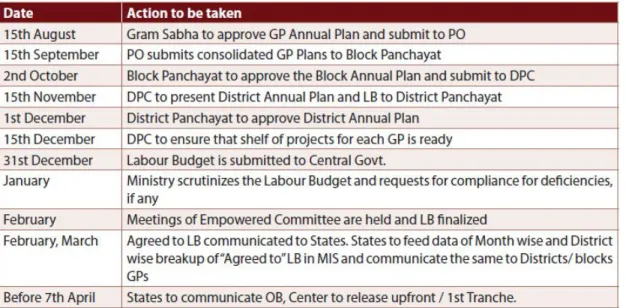
level to the state level and last to the central government (NREGA Operational Guidelines, 2013). This budget plan includes (i) the anticipated quantity of de-mand for jobs in the next year (ii) the precise timing of the dede-mand for work and (iii) a shelf of projects to be prepared and prioritized to meet job demand. Table 1.1 presents the various steps involved in the preparation and finalization of annual labor budgets. Because labor budget is an estimation and NREGA is a demand driven program, the Act states that the States may, based on actual performance, any time during the year, come back to the Ministry requesting revision of their existing labor budget, following the procedures in Table 1.1. However, in fact, the flexibility is limited. Once the labor budget is finalized, the maximum supply of jobs in each state/district/block will not be changed for the next financial year.
Therefore, there will be a shortage of supply for NREGA jobs if any of the following cases occurs—(i) an exogenously fixed maximum level of spending on NREGA by the center government; (ii) an underestimation of job demand in the budget planning; (iii) a poor timing of job demand; and other cases. The ac-tual implementation is further complicated by states’ constraints in organizing projects and workers. Even if the budget planning is not an issue, accommo-dating supply to demand could still be a challenge because of the incapability to meet the relatively skilled labor requirements at the local level, such as pan-chayat technical assistants (Dutta et al., 2014). As a result, although the NREGA program is designed to be a demand-driven program, there is an un-met de-mand for jobs in almost all states (Dutta et al., 2014). On average, each house-hold works roughly 35 person-days per financial year, far less than the claimed 100 days. The extent of the un-met demand differs by districts and by time.
Table 1.1: Timelines for various steps involved in preparation and finaliza-tion of annual labor budget.
Source: Mahatma Gandhi National Rural Employment Guarantee Act 2005 – Operational Guidelines, 4th version. Chapter 6.10.
1.3.3
Landlords and NREGA Employment
In addition to supply constraints in implementing the NREGA, landlords could also affect the supply of public jobs. Providing public jobs to the landless and marginal farmers will increase labor wages (Imbert and Papp, 2015), which will potentially increase production costs for landlords who hire casual labors. Thus this wage effect brings landlords an economic incentive to oppose the imple-mentation of NREGA (Anderson et al., 2015; Maiorano, 2014). There are at least two stages where big landlords can intervene the process of providing NREGA jobs.
First, at the stage of making the labor budget, landlords may lobby against a budget plan that provides enough jobs to the rural poor. As Table 1.1 shows, budget planning is a bottom-top decision making process. The demand for
Table 1.2: Summary statistics of NREGA implementation
(1) (2) (3) (4) (5) 2006 2007 2008 2009 2010 mean/sd mean/sd mean/sd mean/sd mean/sd % of households provided employment 12.40 17.69 27.32 29.63 31.09
(23.01) (25.16) (26.11) (24.22) (23.81) avg days of employment provided per rural SCST person 2.01 2.95 5.24 6.57 6.45
(4.55) (5.07) (6.60) (6.93) (7.12) avg days of employment provided per rural woman 1.25 1.79 3.48 4.32 4.11
(3.66) (3.97) (5.50) (5.90) (5.45) avg days of employment provided per NREGA-woman 19.00 16.35 17.00 21.61 20.84 (16.27) (17.03) (16.80) (15.88) (13.09) labor expense per rural person (2006 Rs.) 68.64 92.41 163.12 175.46 167.70 (192.87) (179.99) (258.53) (224.40) (202.98) number of completed works per 1000 rural persons 1.73 5.06 9.48 13.39 7.68
(5.06) (17.57) (26.09) (20.69) (13.50) # of districts with employemnt provided 122 202 409 410 415
Observations 416 416 416 416 416
Notes: Original data come from MGNREGA public portal. Only districts used in regression analysis are included. Labor expense is deflated by state-wise Consumer Price Index, using 2006 as the base year.
NREGA jobs and the shelf of projects are first identified at the Gram Panchayat level, then the demand and supply are consolidated at the block level, and fur-ther aggregated at the district and state levels. The fact that lower level gov-ernments such as block and village have a substantial discretion in this process renders big landlords’ influences very likely. It is after all easier for landlords to lobby village governments than state governments.
Second, even after labor budget is made, big farmers can still use their po-litical power to block the implementation, such as delaying work assignment, payment and some complementary machinery (see Maiorano (2014) for
anec-dotal evidence of lobbying). As a result, as NREGA annual report shows, the final work completed is smaller than the original budget.
1.4
Mechanism
The political mechanism of inequality and redistribution has been established by the literature. Higher inequality lowers the level of awareness of the poor, de-creasing the level of their political participation (e.g. Bardhan and Mookherjee, 2005; Ramcharan, 2010). Meanwhile, greater inequality can concentrate the ben-efits of political participation and simplify the collective action problem among the landed, which leads to a higher and more effective political participation among the landed elites. In the cases that the landlord elites are a net loser from redistribution, they would block redistribution. Therefore, a higher land inequality predicts lower redistributions to the poor.
As the primary interest of this paper lies in economic effects rather than po-litical effects, I will impose a crude popo-litical mechanism under which landlords have sufficient political power against redistributive policies. Instead, I will fo-cus on the economic incentives that lead big landlords to oppose the provision of public employment.
Providing public jobs to the poor introduces a competition for labor between the public works schemes and the rural private employers. The literature has found that the introduction of NREGA increases rural casual labor wages by 6 percent (Imbert and Papp, 2015). This wage effect could potentially reduce land-lords’ profit, if they keep hiring casual labor. Therefore, the wage-increasing nature of public works schemes provides big landlords the economic incentives
to oppose the program.
1.5
Data
1.5.1
Land Inequality
District-wise data on land distribution in 2005 come from Indian Agricultural Census (excluding Maharashtra), which is conducted at five yearly intervals. Although the information is collected on operational land holdings rather than owned land holdings, the wholly owned and self-operated holdings accounted for 97.14 percent (Page 29, Agriculture Census Report, 2005). Therefore, I use this dataset on operational land holdings to approximate the distributions of land ownership in India.2
This dataset has information on the number and area of operational holdings across the following size bins (in 1000 hectares): below 0.5; 0.5-1; 1-2; 2-3; 3-4; 4-5; 5-7.5; 7.5-10; 10-20; 20 & above. 3 I use the average size of land holdings in each bin to construct land ownership Gini coefficient. The first row of Table 1.3 shows, the average Gini coefficient in our sample districts is 0.47. Figure 1.1 provides state-wise average Gini coefficients in 2005. Figure 1.2 provides the
2According to Agriculture Census in India, “an Operational holder is the person who has
the responsibility for the operation of the agricultural holding and who exercises the technical initiative and is responsible for its operation.” An operational unit could include multiple plots. The operated areas comprise of i) Land owned and self operated; ii) Land leased in; iii) Land otherwise operated.
3I use the information on “Sub-total” land holdings, including both individual holding and
joint holdings, to measure district level land distribution. The ratio of joint holdings to individ-ual holdings is, 1:6.5 in terms of numbers and 1:5 in terms of areas (Agriculture census report 2005, page 121). Land operated by institutions constituted less than 0.5% of the total area, and is excluded from the data.
.1 .2 .3 .4 .5 .6
Gini Coefficient of land inequality
Andaman And Nicobar
Andhra Pradesh
Assam Bihar
Chhattisgarh
Dadra & Nagar Haveli
Goa
Gujarat Haryana
Himachal Pradesh
Jammu And Kashmir
Karnataka
Kerala
Madhya Pradesh
Manipur
Meghalaya Mizoram Nagaland
Odisha Puducherry Punjab Rajasthan Sikkim Tamil Nadu Tripura
Uttar Pradesh Uttarakhand West Bengal
Figure 1.1: Land inequality (Gini coefficient) by state, 2005
Source: The author calculated Gini coefficient based on district-wise land distribution data from 2005 Indian Agricultural census. Only states in the OLS regression sample are included.
shares of operated areas by each decile of holdings. The largest 10 percent of operational holders operate about 46 percent of total land in India. Figure A.2 in Appendix plots the probability distributions of Gini coefficients.4
4There is another relevant fact that supports the legitimacy of using the concentration of land
holdings to proxy for landlords’ political power. According to Agriculture Census Report, 2005 (Page 34), about 96.0 percent of the operational holdings and 94.7 percent of operated areas were operated by village residents whose entire area of land holdings was locating in the village of his residence. These high ratios reduce the concern that big landlords, whose land is in the village but who themselves live outside of the village, might not have the political power to affect NREGA in the current village.
0
.1
.2
.3
Proportion of total land holdings
0 20 40 60 80 100
Percentile of farmers
Figure 1.2: Shares of land area by percentiles of holdings, 2005
Note: Size-classes are as follows: below 0.5; 0.5-1; 1-2; 2-3; 3-4; 4-5; 5-7.5; 7.5-10; 10-20; 20 & above. The graph is derived by first ranking all land holdings by class size in India, then calculate the share of land operated at each decile.
1.5.2
NREGA Implementation
NREGA implementation data come from public data portal5. Table 1.2 presents summary statistics of NREGA implementation by financial year (starting from April in the current year and ends in March the next year) using alternative measurements. The first row tells that, among all working population in India, 12% of them worked for at least one day in public works in 2006, the first year that NREGA was introduced. This number increased to 18% in 2007, and 30% in 2010.
Labor expenses are deflated by state-level consumer price index, using 2006 as the base year. The average wages per rural person received (regardless of their work status in NREGA) increased from 68 Rupees in 2006 to 167 Rupees
in 2010. Figure A.1 in Appendix plots probability distributions of per capita la-bor expenditure. When focusing only on the subpopulation that were provided public employment, the average wages that each household received increased from 2667 Rupees in 2006 to 2867 Rupees in 2010.
Information on the three-phased roll-out comes from the document by NREGA Report (2007)6. Phase 1 include 200 districts, phase 2 includes 130 districts and phase 3 includes the rest of districts. Phases are determined based on the ranking of Backwardness Index (Zimmermann, 2012). I extract this index and its five components from Indian Planning Commission 2003 Report, includ-ing agricultural wages in 1996, agricultural productivity per person 1990-93, agricultural productivity per hectare 1990-93, ratio of SC/ST in the population from 1991 census and poverty ratio 1994 (Commission et al., 2003).
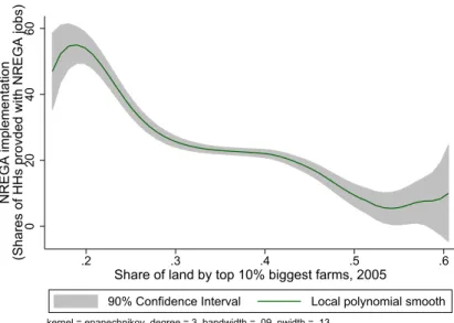
I motivate this paper by observing substantial heterogeneity of NREGA im-plementations across districts. Therefore, it’s important to show variations of both NREGA and land inequality across districts. Figure 1.1 and Figure 1.3 present state level variations of public works provision and land inequality. Fig-ure 1.4 visually presents a negative relation between land inequality and public works provision by doing a kernel regression of the shares of households pro-vided with public jobs on the share of land occupied by top 10% biggest farms.
1.5.3
Demographic and Geographic Information
District profiles are downloaded from 2001 population census, including caste composition, employment and industry structure, literacy rate, amenities and
6This online document nicely presents the phase-in progress http :
0 1 2 3 4 5
Household participation rate (log)
Andaman And Nicobar
Andhra Pradesh
Assam Bihar
Chhattisgarh
Dadra & Nagar Haveli
Goa
Gujarat Haryana
Himachal Pradesh
Jammu And Kashmir
Karnataka
Kerala
Madhya Pradesh
Manipur
Meghalaya Mizoram Nagaland
Odisha Puducherry Punjab Rajasthan Sikkim Tamil Nadu Tripura
Uttar Pradesh Uttarakhand West Bengal
Figure 1.3: Shares of Households provided with NREGA employment by state, 2006-2010
Note: Shares are calculated as total number of households provided with NREGA employment divided by total rural households in the district. All districts in the OLS regression sample are included.
infrastructural facilities, district area size and so on. Population between 2001 and 2010 are filled using these two years’ census data, assuming a growth rate equal to that during 1991-2001. Table 1.3 presents summary statistics of district-wise demographic information in 2005.
The monthly rainfall data are obtained from Center for Climatic Research, University of Delaware. Indian agricultural year is split into two distinct seasons– wet season (from June to November) and dry season (from Decem-ber to May). Existing studies document that NREGA participation is strongly associated with rainfall shocks in wet season. Therefore, I compute wet
sea-0
20
40
60
NREGA implementation
(Shares of HHs provded with NREGA jobs) .2 .3 .4 .5 .6
Share of land by top 10% biggest farms, 2005
90% Confidence Interval Local polynomial smooth
kernel = epanechnikov, degree = 3, bandwidth = .09, pwidth = .13
Figure 1.4: Local polynomial smoothing
Note: Author calculates the share of land by top 10% biggest farms based on 2005 India Agricultural census. NREGA implementation is measured by the share of households provided with public jobs. Kernel = epanechnikov, degree=3, bandwidth=.09.
son precipitation by aggregating the amount of precipitation between June and November in the study year. Figure A.4 in Appendix presents annual rainfall deviation in the country. Soil information is obtained from Food and Agricul-ture Organization (FAO) Digital Soil Map of the World and Derived Soil Prop-erties (CDROM). I map geographical coordinates to district level soil texture. Table 1.3 shows that 91% of the land contains medium or fine level soil; 9% of land is covered by course soil.
Compiling these data sets into a district-wise panel is complicated by district jurisdictional changes during 2001-2011. There were 640 districts in 2011, as opposed to 593 districts in 2001 (Census, 2011). In the analysis, districts with boundary changes are excluded, although results are robust to adding these
Table 1.3: Descriptives of land inequality and demographic information
mean sd min max
Gini coef. 0.47 (0.08) 0 1
Rural area (Sq. km) 5044.34 (4862.42) 119 45382 wet season rainfall (100 mm) 1.03 (0.69) 0 6 % of land covered in fine soil 20.08 (24.19) 0 97 % of land covered in medium soil 70.70 (27.68) 0 100 % of Rural pop 77.94 (15.42) 12 100 Literacy rate 65.29 (11.70) 31 97 % of SC population 15.84 (8.84) 0 50 % of ST population 15.89 (26.18) 0 98 Work-population ratio 40.91 (6.98) 24 63 % of Main workers 30.68 (5.95) 17 52 % of Marginal workers 10.23 (4.20) 2 24 % of Agricultural labourers 22.63 (12.98) 1 63 % of Cultivators 37.77 (18.04) 1 82 % of Household industry workers 4.05 (3.89) 1 31 % of Other industries 35.60 (17.71) 8 91 % villages with Safe Drinking water 96.19 (10.49) 24 100 % villages with Electricity (Power Supply) 84.76 (18.89) 10 100 % villages with Paved approach road 60.87 (25.51) 12 100 % villages with Primary school 84.35 (14.15) 31 100 % villages with Medical facility 41.82 (25.66) 3 100 % villages with Post and telephone facility 52.43 (26.81) 4 100
Observations 416
Total workers = main workers + marginal workers = Ag laborers + cultivators + household in-dustry workers + Other workers. Main workers were those engaged in any economically pro-ductive activity for 183 days or more during the year. Marginal workers were those who worked for less than 183 days. A person was considered as cultivator if he or she was engaged either as employer, single worker or family worker in cultivation of land owned or held from government (or private persons, institutions). A person was regarded as an agricultural labourer if she/he worked in another person’s land for wages in cash, kind or share.
districts back. The final sample includes 416 districts at 2001 district level.7
1.6
Empirical Model and Results
1.6.1
OLS Results
I examine the effect of land inequality on public works provision by pooling the NREGA implementation data during 2006-2010 and using across district (within-state) variations of land concentration in 2005.8 The model specification is:
Yit =α0+β∗IN Ei,2005+αXit+αsDstate+αtDt+εit,∀t ∈ {2006,2007,2008,2009,2010}
(1.1) whereβis the coefficient of interest.
IN Ei,2005 denotes land inequality in district iin 2005, measured by Gini co-efficient (in logarithm). Yitdenotes the implementation of the NREGA program
in district i in year t, measured by proportions of rural households provided with NREGA employment (in logarithm). A negative sign ofβmeans NREGA job provision is negatively associated with land inequality. Standard errors are clustered at the district level.
7This seemingly much smaller number relevant to total Indian districts is a consequence of
combining different data sources, each of which has some missing districts. First, 2005 Agricul-ture Census only contains 528 districts (as Maharashtra state is not included), about 90 of which are either newly created or the original districts that got split. These 90 districts are dropped when I combine Agriculture census to 2001 population census. Second, 26 districts that are in-cluded in Agriculture census are not inin-cluded in NREGA public portal (and this public portal posts information at 2010 district level). Third, about 10 districts lack information on soil quality or rural area size etc that further reduces the number of observations. In the end, we have 416 districts for each year at 2001 district level.
8Table A.2 shows that land distribution didn’t change at statistically significant level during
To identify the effect of the concentration of land ownership on public works provision, β, I need to control for variables that are correlated with land in-equality and at the same time affect NREGA implementation. The first set of confounding factors contains the capacity of local governments to accommo-date job supply to job demand. As mentioned in the previous section, although central government bears most of the cost, it does not imply there will be zero cost to local governments when employing workers under NREGA. The imple-mentation cost may be particularly high in poor districts (Dutta et al., 2014). Therefore, I control for variables reflecting the level of local economic devel-opment to capture local governments’ accommodation capability, such as the percentage of villages that have access to drinking water, electricity, paved road and schools in the district and other rural infrastructure variables.
In the same vein, I also control for “Backwardness Index”, a score con-structed by Indian planning commission in 2003, with smaller numbers mean-ing bemean-ing more backward. The literature has shown that NREGA program rolls out from backward districts to more affluent districts, in the order of their rank-ings on this index(Zimmermann, 2012; Dasgupta et al., 2017). However, this roll-out rule is not absolutely enforced, reflected by the fact that many Phase 2 districts have smaller values of backwardness index than Phase 1 districts. Therefore, I also include phase dummies to capture the heterogeneous imple-mentation by phases.
In addition, the model also includes soil texture and the current wet sea-son’s rainfall deviations from historical means, because these geographic vari-ables could affect both the demand for and the supply of NREGA jobs, and are also documented to be associated with land distribution. 9 I also include a
tor of state dummy,Dstate, and year dummy, Dt, restricting the cross-sectional
comparisons to within-state variations.
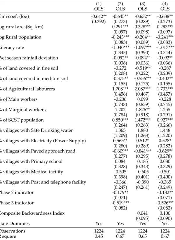
The results of OLS estimates are presented in Table 1.4. It gives a significantly negative relation between Gini coefficient and the proportion of rural house-holds provided with NREGA employment. The results are robust to adding extra covariates. Column 4 suggests, districts with a 1% (or in absolute term, 0.0047) higher Gini coefficient would have 0.6% (or in absolute term, 0.006 * 30=1.8 percentage points) fewer households provided with NREGA jobs.
1.6.2
Addressing Endogeneity
OLS estimates cannot be interpreted as causal. The most apparent threat is reverse causality, as redistributive policies such as public works schemes also shape inequality. Using land inequality in 2005 (much ahead of the initiation of NREGA) allows for some control of potential reverse causality (i.e. it’s rea-sonable that land inequality in 2005 will affect public work provision in post-2006, but unlikely that public works in post-2006 will affect land inequality in 2005). However, the model will still capture some endogeneity issues if there are some omitted variables which are correlated with both land ownership and the demand/supply side of NREGA implementation. For instance, adverse ge-ographical and climatic characteristics may concentrate land ownership by
re-is establre-ished by exre-isting studies that use various geographical conditions to instrument for land inequality, including climatic information, soil quality and the share of cash crop (inequality-rising) and wheat/rice crop etc. (e.g. Easterly, 2007; Sokoloff and Engerman, 2000; Galor et al., 2009; Ramcharan, 2010; Cinnirella and Hornung, 2016; Baten and Juif, 2014). The spirits of these IVs are, small farmers are usually less able to hedge against negative weather shocks, and have a smaller demand for land in areas with poor soil quality (or in areas with violent rainfall variability). Thus, regions with poorer soil quality (or more rain variability) have higher land concentration.
Table 1.4: Dep var: % of households provided with NREGA jobs (OLS)
(1) (2) (3) (4)
OLS OLS OLS OLS
Gini coef. (log) -0.642** -0.645** -0.632** -0.638** (0.292) (0.273) (0.289) (0.273) log rural area(Sq. km) 0.291*** 0.328*** 0.293***
(0.097) (0.098) (0.097) log Rural population -0.243*** -0.204** -0.241***
(0.083) (0.089) (0.083)
Literacy rate -1.040*** -1.097*** -1.017***
(0.345) (0.390) (0.344) Wet season rainfall deviation -0.092** -0.094** -0.092**
(0.036) (0.036) (0.036) % of land covered in fine soil -0.272 -0.519** -0.287 (0.208) (0.222) (0.209) % of land covered in medium soil -0.375** -0.556*** -0.402**
(0.155) (0.175) (0.155) % of Agricultural labourers 1.708*** 2.087*** 1.733*** (0.456) (0.467) (0.457) % of Main workers -0.206 0.099 -0.228 (0.748) (0.839) (0.745) % of Marginal workers 1.202 1.826** 1.255 (0.784) (0.918) (0.791) % of SCST population 0.850*** 1.472*** 0.927*** (0.264) (0.263) (0.266) % villages with Safe Drinking water 1.365 1.880 1.448
(1.209) (1.263) (1.220) % villages with Electricity (Power Supply) 0.565** 0.512* 0.528* (0.280) (0.289) (0.282) % villages with Paved approach road -0.609** -0.841*** -0.629**
(0.277) (0.295) (0.278) % villages with Primary school 0.084 0.185 0.080
(0.328) (0.343) (0.329) % villages with Medical facility -0.505 -0.605 -0.501 (0.398) (0.401) (0.400) % villages with Post and telephone facility -0.366 -0.390 -0.365 (0.247) (0.261) (0.249)
Phase 2 indicator -0.179** -0.182**
(0.071) (0.071)
Phase 3 indicator -0.519*** -0.526***
(0.082) (0.082)
Composite Backwardness Index 0.041 0.100
(0.095) (0.090)
State Dummies Yes Yes Yes Yes
Observations 1224 1224 1224 1224
R square 0.45 0.67 0.65 0.67
Notes: Dependent variable is the logarithm of the share of households provided with NREGA jobs in the district. Standard errors are in parentheses, clustered at district level. * p<0.10, ** p<0.05, *** p<0.01.
ducing the demand for land by marginal farmers9 ; and meanwhile adverse geographical and climatic characteristics may increase the demand for NREGA jobs and decrease the government capability to supply jobs. Although I have included the covariates of soil texture and rainfall variations, if there are other such geographical and climatic variables omitted, OLS estimates will be biased (upward and toward zero in the given example). In addition to omitted variable bias, there is also measurement error of land distribution, which will lead to the attenuation bias of the estimates.
I address the endogeneity issues by taking advantage of historical institu-tions in India — land revenue collection system, established by British colo-nial rulers during 1750-1861. This variable is constructed based on the study by Banerjee and Iyer (2005). Land revenue, or land tax, was the major source of government revenue in India and during British times as well. British admin-istration established three systems to collect land revenue in all cultivable land in British India: (a) landlord-based system, where the liability for a village or a group of villages lay with with a single landlord; (b) an individual cultivator-based system, where revenue settlements was made directly with individual cultivators; (c) village-based system, where village bodies which jointly owned the village were responsible for the land revenue. Figure A.3 in the appendix presents the map of these three different land revenue systems in British India. System (c), village-based system, could be further grouped as either system (a) or (b), depending on whether the village body was a single landlord or a large number of members with each person being responsible for a fixed share of the revenue. Table 1.5 presents state-wise distribution of landlord and non-landlord districts.
Table 1.5: State-wise distribution of landlord and non-landlord districts
Landlord Non-landlord Total districts Mean landlord proportion
Andhra Pradesh 2 8 10 0.34 Bihar 1 0 1 1 Chhattisgarh 4 1 5 0.80 Gujarat 0 6 6 0 Haryana 0 4 4 0.15 Karnataka 0 11 11 0 Madhya Pradesh 10 1 11 0.89 Odisha 6 2 8 0.68 Punjab 0 5 5 0.14 Rajasthan 1 0 1 1 Tamil Nadu 2 9 11 0.28 Uttar Pradesh 12 34 46 0.59 Uttarakhand 0 3 3 0.38 West Bengal 10 0 10 1 Total 48 84 132 0.51
Source: This is a subsample of districts from the study by Banerjee and Iyer (2005).
To identify a causal relation between land distribution and the provision of public works under NREGA, I use the binary indicator of land revenue system — whether this district was a landlord district in British India — to instrument for land inequality in 2005. The instrumental variable strategy relies on the as-sumption that land revenue collection system under British India only affects redistributive policies through contemporary and current land inequality, after controlling for all observables. This is plausible because the way that British colonial rulers decided land revenue system in different areas was not based on
0 2 4 6 8 10 Probability Distribution .3 .4 .5 .6 Gini coefficient
Nonlandlord districts Landlord districts
Figure 1.5: Visualize first stage —Land Inequality (Gini coefficient) in landlord/non-landlord districts
Source: The author calculated land ownership Gini coefficient based on 2005 India Agricultural census.
a hard rule, i.e. in terms of land fertility, weather or labor productivity (Baner-jee and Iyer, 2005). Figure 1.5 visually presents the negative relation between landlord-dominated revenue collection system and current land inequality.
I estimate first stage relation using the following equation:
IN Ei,2005 =α00+ρZi+α0Xit+α0sDstate+α0tDt+ηit (1.2)
whereZiis the binary indicator that equals to 1 if districtiused to be a
landlord-dominated district in British India, and zero otherwise;IN Ei,2005 denotes land inequality in districtiin 2005, measured by Gini coefficient;Xidenotes the same
vector of district-wise covariates as in Equation(1.1).10
10By restricting the variations to be within-state, in this IV estimation, states where land tenure
systems don’t vary across districts within the state will be absorbed in the state fixed effects, such as Bihar, Gujarat, Haryana, Karnataka, Punjab, Rajasthan, Uttarakhand and West Bengal. As a result, 91 districts in 6 states are left and contribute to the variations in the IV estimation.
.48
.5
.52
.54
.56
Share of land by top 10 percent farms
1950 1960 1970 1980 1990
Year
Non-Landlord districts Landlord districts
Figure 1.6: Trends of Land Inequality (share of land by top 10% land hold-ings) in landlord/nonlandlord districts
Source: Land reform data during 1957-1992 are from (Besley and Burgess, 2000). Data on Land revenue system are from (Banerjee and Iyer, 2005).
The first-stage conditional correlations suggest that landlord-dominated dis-tricts have 7.4% lower Gini land ownership inequality in 2005 (Table 1.6). This estimated effect is equivalent to -0.035 (= -7.4% * 0.47) in absolute term of gini coefficient, or 0.5 (=0.035/0.08) standard deviation of gini coefficient, consid-ering that the mean and standard deviation of Gini coefficient are respectively 0.47 and 0.08 in the sample.
The first-stage result that previously landlord-dominated districts in British India has a lower land inequality today is consistent with the study by Banerjee and Iyer (2005). They show that states with a higher landlord proportion had higher Gini measures of land ownership inequality in 1885, and this inequality
persisted until the end of the colonial period11. However, as they argue, ma-jor landlord-dominated states enacted 6.5 land reforms in the period between 1957-1992, while non-landlord states had an average of 3.5. According to Besley and Burgess (2000), states that enacted a larger number of land reforms had a greater decline of Gini coefficient of land inequality. Therefore, with this chain of reasoning, landlord district saw a greater decline of land inequality than non-landlord districts, driven by a great number of land reforms after Indian Inde-pendence. Furthermore, the negative sign of first-stage results is consistent with the study by (Besley et al., 2016) that shows in the long-run land inequality is lower in areas that saw greater intensity of tenancy reform.
I then plot the numbers of land reforms over time in major landlord and non-landlord states in Figure 1.7, which provides consistent evidence with the litera-ture that landlord areas enacted more frequent land reforms than non-landlord areas.12 To depictwhenland ownership distribution in landlord dominated dis-tricts started to become more equal than non-landlord dominated disdis-tricts, I further plot the trends of land inequality, measured by the share of land owned by the top 10% land holdings, for major landlord and non-landlord districts in Figure 1.6.13 It shows that the shift of landlord districts from having relatively high land inequality to relatively low land inequality occurred in 1970.
Inter-11 Banerjee and Iyer (2005) explains why the choice of landlord revenue system had a strong
effect on the distribution of land and wealth in British India period. “Under landlord-based systems, the landlords were given a more or less free hand to set the terms for the tenants and, as a result, they were in a position to appropriate most of the gains in productivity.”
12I calculate these two series of numbers by combining state-wise land reform data
from (Besley and Burgess, 2000) into the current district-wise sample. Major landlord-dominated areas are states with an above-median share of districts belonging to landlord dom-inated districts.
13Ideally, I need district-wise land inequality to plot the changes of land inequality over time
in landlord versus non-landlord districts. However, the lack of district-wise land distribution data prevents me from doing so. Instead, by combining with state-wise data on land reform and land distribution from Besley and Burgess (2000), I plot these trends for major landlord states and non-landlord states, where landlord states are defined as states with an above-median share of districts belonging to landlord dominated districts, and non-landlord states.
estingly, this turning point coincides with the time when major landlord states started to outnumber non-landlord states in land reforms as shown in the Fig-ure 1.7. All such information together explains the negative sign of first-stage estimate—landlord districts, although starting with higher land inequality in British Indian period, enacted more land reforms after Indian Independence, and hence ended up having lower land inequality in 2005.
The instrumental variable strategy relies on the assumption that land rev-enue collection system under British India only affects redistributive policies through contemporary and current land inequality, after controlling for observ-ables. However, if different historical property rights institutions lead to persis-tent unobserved culture and institutional outcomes, and such unobserved out-comes are also correlated with redistributive policies, then this IV would violate the exclusion condition. I will examine the sensitivity of the estimations to the degree in which the exclusion restriction is potentially violated using sensitivity analysis proposed in Conley et al. (2012).
1.6.3
IV Results
Table 1.7 presents two-stage least square (2SLS) estimations of the effect of land inequality on NREGA implementation (measured by proportions of household provided with NREGA jobs). The sample size drops to one third of the origi-nal size, because the instrumental variable, landlord versus non-landlord domi-nated districts indicator, is only defined in districts that were under British India during 1850-1947.
Table 1.6: Dep var: Land inequality (gini coefficient) in 2005, (First stage)
(1) (2) (3) (4)
OLS OLS OLS OLS
Landlord district indicator -0.079*** -0.082*** -0.074*** -0.074*** (0.021) (0.020) (0.020) (0.020)
log rural area(Sq. km) 0.037 0.043 0.041
(0.031) (0.030) (0.028)
log Rural population -0.010 -0.021 -0.020
(0.040) (0.036) (0.037)
Literacy rate -0.013 -0.002 -0.006
(0.125) (0.108) (0.122) Wet season rainfall deviation -0.007** -0.007** -0.007**
(0.003) (0.003) (0.003) % of land covered in fine soil -0.478*** -0.490*** -0.495***
(0.073) (0.067) (0.072) % of land covered in medium soil -0.243*** -0.259*** -0.263***
(0.059) (0.056) (0.057) % of Agricultural labourers 0.144 0.178* 0.181* (0.101) (0.097) (0.100) % of Main workers 0.558** 0.485** 0.489** (0.231) (0.209) (0.225) % of Marginal workers 0.081 0.122 0.100 (0.296) (0.261) (0.296) % of SCST population -0.110 -0.065 -0.063 (0.114) (0.106) (0.116) % villages with Safe Drinking water -0.433 -0.408 -0.368
(0.410) (0.388) (0.416) % villages with Electricity (Power Supply) -0.031 -0.046 -0.047
(0.092) (0.089) (0.092) % villages with Paved approach road 0.171** 0.161** 0.165** (0.083) (0.077) (0.080) % villages with Primary school 0.127 0.117 0.112
(0.092) (0.085) (0.085) % villages with Medical facility 0.011 0.009 0.007
(0.057) (0.059) (0.058) % villages with Post and telephone facility 0.001 0.003 0.004
(0.070) (0.068) (0.067) Phase 2 indicator -0.002 -0.005 (0.021) (0.021) Phase 3 indicator 0.010 0.000 (0.023) (0.022) Backwardness Index 0.067*** 0.066*** (0.018) (0.017)
State Dummies Yes Yes Yes Yes
Observations 570 570 570 570
R square 0.63 0.80 0.81 0.81
F test: landlord indicator coef=0 14.21 17.13 14.12 14.28
Notes: “Landlord district indicator” equals 1 if the district in question was a landlord district (i.e. landlords were responsible for collecting land revenue) in British Raj. Land Gini coefficient is constructed using 2005 Indian Agricultural census. All models include year dummy. Standard errors are clustered at district level. * p<0.10, ** p<0.05, *** p<0.01.
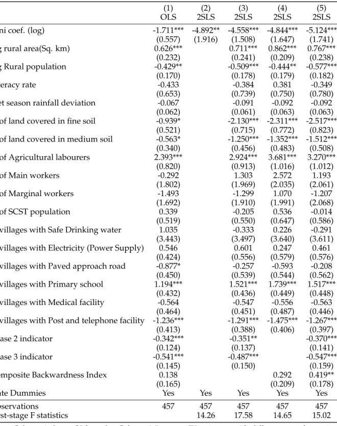
a full set of control variables, as a reference to 2SLS estimates. It suggests that a 1% increase in gini coefficient of land ownership is associated with a 1.7% (or equivalent to 0.5 percentage points, given that the average share of households provided with NREGA jobs is 30%) decrease of the share of households pro-vided with NREGA jobs. Column 2-5 present IV estimates with different sets of covariates added. First-stage F statistics are all above 10, suggesting a rejec-tion of weak instrument null hypothesis. The size of the point estimate for the Gini coefficient is relatively stable over the last four IV specifications, suggesting that a 1% increase in gini coefficient of land ownership would have decreased the share of households provided with NREGA jobs by 5% (or equivalent to 1.5 percentage points, given that the average share of households provided with NREGA jobs is 30%).
Column 3 in Table 1.7 adds various variables that reflect the demand for and the supply of NREGA jobs. It suggests soil quality and some rural infras-tructure are negatively associated with public works provision. For instance, a 1% higher proportion of land covered by fine soil rather than coarse soil in the district is associated with a 2% lower participation by households. Similarly, a 1% higher proportion of villages having access to post and telephone facility is associated with a 1% lower participation by households. Such evidence is consistent the demand-driven nature of NREGA — areas with favorable agri-cultural conditions may not need the job protection by NREGA, because there are already enough jobs in rural labor market. The negative relation may also be because the central government allocates less public employment in those relatively better endowed and more developed areas.
Table 1.7: Dep var: % of households provided with NREGA jobs
(1) (2) (3) (4) (5)
OLS 2SLS 2SLS 2SLS 2SLS
Gini coef. (log) -1.711*** -4.892** -4.558*** -4.844*** -5.124*** (0.557) (1.916) (1.508) (1.647) (1.741) log rural area(Sq. km) 0.626*** 0.711*** 0.862*** 0.767***
(0.232) (0.241) (0.209) (0.238) log Rural population -0.429** -0.509*** -0.444** -0.577***
(0.170) (0.178) (0.179) (0.182)
Literacy rate -0.433 -0.384 0.381 -0.349
(0.653) (0.739) (0.750) (0.780) Wet season rainfall deviation -0.067 -0.091 -0.092 -0.092 (0.062) (0.061) (0.063) (0.063) % of land covered in fine soil -0.939* -2.130*** -2.311*** -2.517***
(0.521) (0.715) (0.772) (0.823) % of land covered in medium soil -0.563* -1.250*** -1.352*** -1.512***
(0.340) (0.456) (0.483) (0.508) % of Agricultural labourers 2.393*** 2.924*** 3.681*** 3.270*** (0.820) (0.913) (1.016) (1.012) % of Main workers -0.292 1.303 2.572 1.193 (1.802) (1.969) (2.035) (2.061) % of Marginal workers -1.493 -1.299 1.070 -1.207 (1.692) (1.910) (1.991) (2.068) % of SCST population 0.339 -0.205 0.536 -0.014 (0.519) (0.550) (0.647) (0.586) % villages with Safe Drinking water 1.035 -0.333 0.226 -0.291 (3.443) (3.497) (3.640) (3.611) % villages with Electricity (Power Supply) 0.546 0.601 0.247 0.461
(0.424) (0.556) (0.579) (0.576) % villages with Paved approach road -0.877* -0.257 -0.593 -0.208 (0.450) (0.539) (0.544) (0.562) % villages with Primary school 1.194*** 1.521*** 1.739*** 1.517***
(0.432) (0.436) (0.449) (0.448) % villages with Medical facility -0.564 -0.547 -0.556 -0.563 (0.464) (0.451) (0.487) (0.446) % villages with Post and telephone facility -1.236*** -1.291*** -1.475*** -1.267***
(0.413) (0.388) (0.406) (0.397)
Phase 2 indicator -0.342*** -0.351** -0.370***
(0.124) (0.137) (0.141)
Phase 3 indicator -0.541*** -0.487*** -0.547***
(0.145) (0.150) (0.159)
Composite Backwardness Index 0.138 0.292 0.419**
(0.165) (0.209) (0.178)
State Dummies Yes Yes Yes Yes Yes
Observations 457 457 457 457 457
First-stage F statistics 14.26 17.58 14.65 15.02
Notes: Column 1 shows OLS results; Column 2-5 present IV estimates with different sets of covariates added. Dependent variable is proportions of household provided with NREGA jobs in each year 2006-2010. District-wise land Gini coefficient is constructed using 2005 Indian Agricultural census. Instrumental vari-able is a binary indicator that equals 1 if the district in question was a landlord district (i.e. landlords were responsible for collecting land revenue) in British Raj. All models include year and state dummy. Standard
group. The estimated coefficients of Phase 2 and Phase 3 indicator are both neg-ative, with the former having a smaller magnitude than the latter. This suggests that Phase 1 districts have the highest level of public employment provided, followed by Phase 2 districts and then Phase 3 districts. This relative position resonates with the fact that NREGA rolls out from the most backward districts to richer districts.
Column 4 replaces Phase dummies with “Backwardness Index”, which cap-tures how the program was rolled out. Column 5 adds both Phase dummies and Backwardness Index. Backwardness Index (a greater value indicating economi-cally more developed) is expected to be negatively related to job provision, be-cause more NREGA jobs are demanded in backward areas. However, both col-umn 4 and colcol-umn 5 suggest a positive relation between this index and NREGA job provision, although not at a statistically significant level. This positive rela-tion may be because the higher demand in the backward areas is dominated by the lower capacity to accommodate NREGA projects. In addition, the magni-tude of the estimated effect of land inequality on NREGA provision is slightly bigger in column 5 than that in column 3.
To put these results into perspective, consider the difference between land inequality Gini coefficient in two districts in Uttar Pradesh, Ballia and Alla-habad. In Ballia, gini coefficient of land ownership was 0.486 (which is at the 50th percentile of the distribution of gini coefficient) in 2005, and in Allahabad, this number is 0.519 (which is at the 80th percentile). Using the estimates in col-umn (5), the difference of 0.033 points, or 6.6% (= 0.033/0.518), in gini coefficient implies that 33% (=6.6 * 5 % ) more households would have been provided with NREGA jobs in Allahabad if it had a land gini coefficient as small as Bellia’s.