An Optimal Algorithm for Coverage Hole Healing
in Hybrid Sensor Networks
Dung T. Nguyen, Nam P. Nguyen, My T. Thai, Abdelsalam Helal
Department of Computer and Information Science and Engineering, University of Florida Email: {dtnguyen, nanguyen, mythai, helal}@cise.ufl.edu
Abstract—Network coverage is one of the most decisive factors
for determining the efficiency of a wireless sensor network. However, in dangerous or hostile environments such as battle fields or active volcano areas, we can neither deterministically or purposely deploy sensors as desired, thus the emergence of coverage holes (the unmonitored areas) is unavoidable. In addition, the introduction of new coverage holes during network operation due to sensor failures due to energy depletion shall significantly reduce coverage efficacy. Therefore, we need to either remotely control or set up a protocol to heal them as soon as possible in an automated fashion.
In this paper, we focus on how to schedule mobile sensors in order to cope with coverage hole issues in a hybrid sensor network containing both static and mobile sensors. To this end, we introduce a new metric, namely to maximize the minimum remaining energy of all moved sensor since the more energy remains, the longer the network can operate. Based on this metric, we propose an efficient coverage healing algorithm that always determines an optimal location for each mobile sensor in order to heal all coverage holes, after all mobile sensors locations and coverage holes are located. Simulation results confirm the efficiency and utilization of our proposed method.
Index Terms—hybrid sensor network; coverage hole,
move-ment schedule, mobile sensor, coverage hole healing I. INTRODUCTION
Wireless sensor networks (WSN) have been developing quickly in the recent decade due to their low costs and wide ranges of applications. Autonomous sensors can be deployed in an area and incorporate to each other to fulfill a specific task such as habitat monitoring, environment observation or battle field surveillance [1]. A sensor can only sense and detect events within its sensing range which usually forms a circle centered at its location. The union of areas monitored by all sensors is defined as the covered area of the whole network. To guarantee the monitoring quality, it is crucial that every single point in the target field must be within the network’s covered area, or in other words, every point in the target field must be monitored by at least one sensor.
The development of sensing coverage holes, i.e., unmoni-tored areas, during network deployment and operation is one of the most difficult problems to address. In many dangerous and hostile regions such as battle fields or active volcano areas, we can neither deterministically nor purposely deploy sensors, we can only do so randomly. However, a notable problem with random sensor deployment is the unbalance of sensor density in the targeting area: the sensor density could be high in some subareas but might be extremely low in some of the others, thus coverage holes are more likely to emerge in those regions. Therefore, the development of coverage holes is unavoidable.
Additionally, during network operation, some sensors may accidentally stop working due to either energy depletion or failure under some adversarial events. Therefore, it is crucial to have a mechanism for not only setting up and maintaining network coverage but also healing the sensing holes as soon as they arise in an automated manner. This is an interesting, yet changeling problem in WSN.
In this paper, we investigate the coverage healing problem in a hybrid sensor network containing both static and mobile sensors. Wang [2] proposed an economical deployment strat-egy for this type of networks that uses only a small fraction of mobile sensors to save many static sensors. In this type of networks, mobile sensors can be used to heal coverage holes. Assume that the locations of coverage holes and mobile sen-sors are already detected, the coverage healing problem asks for a movement scheduling that relocates all or some of the mobile sensors to their appropriate locations in order to cover all holes. Wang [2] designed an algorithm for this problem with an objective of minimizing the total consumed energy of mobile sensors. However, this objective has a shortcoming, especially with sensors having the lowest remaining energy: these sensors may unpredictably stop working any time due to lack of energy. This observation drives the need for a better sensor scheduling to heal coverage holes.
To overcome this limitation, we present a new metric to evaluate a sensor movement scheduling: maximize the mini-mum remaining energy over all moving sensors. In particular, we introduce an algorithm which not only provides the optimal solution but also very efficient and easy to implement in practice. In a big picture, our proposed algorithm first tries to attain a possible optimal value of remaining energy and then, based on the gained information, schedules an optimal movement which achieves this value. In some cases, if the number of failed sensors are small and consequently, there are not too many coverage holes to heal, computing the movement schedule of the whole network is of high costs and unnecessary. Therefore, we introduce a simple and efficient distributed scheme to deal with these special cases. This scheme not only requires low computational costs but also quickly locates the appropriate mobile sensors to heal a new hole as soon as its location is detected.
Our main contributions in this paper are threefold. Firstly, we propose an exact O(√nmlogm) algorithm that provides an optimal solution for coverage healing problem on a hybrid sensor network, wherenandmare the numbers of nodes and edges in the underlying bipartite graph. Secondly, we intro-duce a distributed heuristic scheme to quickly and efficiently
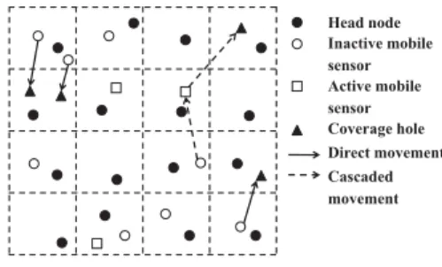
Head node Inactive mobile sensor Active mobile sensor Coverage hole Direct movement Cascaded movement
Fig. 1. Network model
heal coverage holes when not too many of them show up. This heuristic scheme can identify a specific mobile sensor to instantly heal any newly introduced coverage hole with very low message and computational complexity. Thirdly, we extensively test our algorithm on various networks against the one suggested by Wang [2]. Experimental results show that our new metric, maximizing the lowest remaining energy, is more suitable in WSN than the total consumed energy in [2]. In addition, this distributed scheme usually provides near optimal values in most networks.
The rest of the paper is organized as follows: Section II de-scribes the network models and problem statement. Section III presents our algorithm for computing the optimal movement scheduling. A distributed scheme to deal with some special cases is introduced in the Section IV. In section V, we show experiment results. Section VI briefly summarizes the related work, and finally Section VII concludes our work.
II. NETWORKMODEL ANDPROBLEMFORMULATION A. Network model
A hybrid sensor network consists of both static and mobile sensors working together in a targeted field. Each sensor is powered by a different amount of energy and has its own com-munication as well as sensing range. When a mobile sensor moves to a new location, it consumes energy proportionally to the distance traveled. In our model, each sensor is able to estimate its remaining energy thanks to the method suggested in [3] and identify its current location by the equipped GPS device [4].
There are two types of mobile sensors during network oper-ation: activeandinactive mobile sensors. Active mobile sen-sors are those actually working in the field and in cooperation with the other sensors to monitor the target area. In contrast, inactive ones are mobile sensors in the sleeping mode. In addition, there is a base station equipped with rich computing resources to manage the network and exchange information with the remote controller. Sensors gather monitored data and other network information and send them back to the base station for processing. The base station then sends back control messages to sensors.
For the ease of management, the target area is divided into autonomous subareas (called cells) of the same size as illustrated in Fig. 1. Each subareas is controlled by a head node which manages activities within its cell. In fact, a head node is a regular designated sensor and any sensor in the cell can take the role of the head node. In our model, sensors
within a cell will take turn to be the head node. In particular, a head node knows the following information within its area (1) Static and mobile sensor locations and (2) Coverage hole locations. Furthermore, for each mobile sensor, the following information is made available to the head node: its remaining energy and working status (active or inactive).
The size of a coverage hole in our model can be estimated using the proposed method in [5]. This implies the number of mobile sensors for healing the hole can be estimated approximately from the size of the hole and their sensing ranges. In this paper, we assume that any newly introduced coverage hole can be covered by a single mobile sensor. This assumption makes sense since any large coverage hole can be decomposed as a collection of smaller ones, in which each hole can be fully monitored by a sensor. When a sensor detects a hole near it, it sends information to the head node. Thus, the information of coverage holes in a grid is made available to the head node as well as the base station.
B. Coverage Hole Healing Problem
After the network is deployed, two important tasks are main-taining its coverage and healing coverage holes as soon as they arise. Generally, one would expect that the network will work stably and last as long as possible. This means the rearranged mobile sensors, after the hole healing process, should have as much remaining energy as possible. However, since sensing holes can simultaneously and unpredictably appear at different regions in the targeting area, how can we quickly find an optimal movement scheduling for mobile sensors satisfying the above network requirements? Informally, the Coverage Hole Healing Problem asks for a sensor scheduling that not only heals all introduced coverage holes but also maximizes the lowest remaining energy over all moving sensors, assuming the knowledge of holes’ locations.
Cascaded Movement: There are two possible scenarios when a mobile sensor is ordered to move to a new location. An inactive one simply moves directly to the desired location whereas an active one may require an extra consideration: any active mobile sensor immediately creates a new hole behind itself as soon as it moves to a new location. Clearly, that hole needs to be covered by another mobile sensor and the movement of that sensor may further lead to another uncovered hole as a result. These actions reassemble the concept of a cascaded movement of mobile sensors on WSN.
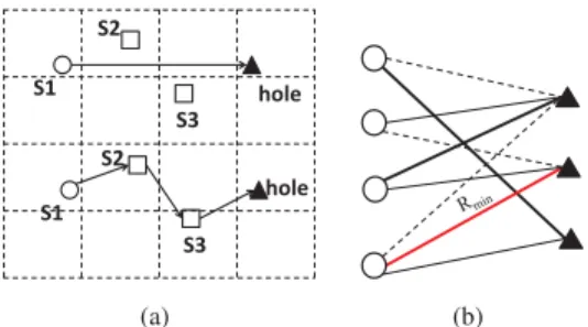
Cascaded movement represents an opportunity in our ap-proach since allowing this will help in significantly reducing the consumed energy of each sensor, thus enhancing its remaining energy. To give a sense of its effect, let us consider the example illustrated in Fig. 2(a). In this example, we have two possibilities. In the first option, we move inactive sensor S1 directly to the hole. In the other option, we can moveS1 to S2’s location, S2 to S3’s location and then move S3 to heal the hole. After all sensors move, it is obvious that the remaining energy of S1 in the first option may be less than the minimum energy ofS1,S2 andS3 in the second option, since S1 has traveled a much longer distance and thus, has consumed much more energy than S2 or S3 has. In other words, the second option provides a better solution than the
first one. A big picture of the whole movement schedule is illustrated in Fig. 1.
The Coverage Hole Healing Problem (CHP) can be formally described as follows: Given a hybrid sensor network with a set M of mobile sensors, a set S of static sensors and a set H of locations of coverage holes, find a scheduling for mobile sensors, allowing cascaded movement, to quickly and efficiently heal the holes in H such that the lowest remaining energy over all moving sensors is maximized.
III. COVERAGEHOLEHEALINGALGORITHM In this section, we present our optimal solution for CHP based on the graph theory approach. Basically, our solution consists of two main steps: 1) construct a bipartite graph G representing the relationship between mobile sensors and coverage holes. 2) Find a complete matching T of G that maximize the lightest weight inT. Based onT, mobile sensors will move to correct location to heal the coverage holes.
A. Building bipartite graph
Based on the gathered information at the base station, we construct a bipartite graph G = ((M, H), E) describing the network and prove that CHP is, in fact, equivalent to finding a complete matching (in terms of holes) onG. We first construct G with directed movement scheduling using only inactive mobile sensors and then, extend Gto capture schedules that allow cascaded movements.
To capture direct movements, Gis constructed as follows: Let M and H be sets of nodes representing inactive mobile sensors and coverage holes, respectively. For any pair of a mobile sensor Mi and a hole Hj, an edge eij is added to
the edge set E if Mi has enough energy to move to Hj.
The weight w(eij) of this edge is the remaining energy of
Mi after moving to Hj. A scheduling that orders mobile
sensors M1, M2, . . . , Mh healing holes H1, H2, . . . , Hh can
be represented by a complete matching{e11, e22, . . . , ehh}on
G, where h =|H|. By constructing this way, the minimum energy remains after a scheduling is indeed the weight of the lightest edge in the matching.
Now we modify Gto allow cascaded movements by intro-ducing a dummy holedhfor each working sensorswsand add dhtoHas well aswstoM. The weights of edges connecting a dummy hole to other mobile sensors are computed the same as others, except for the edge connecting dh to ws whose weight is infinite. This modification transforms the problem back to the case of direct movements.
Lemma 1: The CHP problem is equivalent to finding a
complete matching on G (in terms of coverage holes) that maximizes the weight of the lightest edge.
Proof:We will prove that if the lowest remaining energy is maximized in CHP (say its value isRmin) then there exists
an optimal complete matching on Gwhose the lightest edge weight is exactly Rmin, and vice versa.
Let M S be an optimal movement scheduling in CHP. Denote by Rmin the minimum remaining energy over all
moving sensors. We will construct a complete matching T on G whose lightest edge weight is Rmin. Initialize T =∅.
For each holeHj, if it can be covered by a sensorMi, we add
S1 S3 S2 hole S1 S3 S2 hole (a) (b)
Fig. 2. 2(a): Cascaded movement. 2(b): An optimal matching (shown in thick edges) with mobile sensors on the left and holes on the right. The lowest edge weightRminis shown in red. The removals of edges whose weights are less thanRmin(shown in dotted lines) will not affect the optimal solution edge eij into T. According to the definition of edge weight,
the weight of the lightest edge inT is Rmin. Now, there are
only dummy nodes in H that are not covered by any moved sensor. For each dh, we add an edge connecting dh to its corresponding inactive mobile sensor wsinto T; these edges have weight infinite. Since each hole is covered by one sensor, it implies thatT is a complete matching onGwith the weight of lightest edge is Rmin.
On the other hand, if there exists a complete matching T whose lightest edge weight is Rmin, then for each edge eij
inT, ifHj is not the dummy hole created byMi, moveMi
to heal Hj. Since T is a complete matching, each hole is
healed by exactly one sensor and the minimum energy over all moving sensors isRmin, which completes the proof.
B. Scheduling algorithm
The key idea of our approach is that, ifRminis the weight
of the lightest edge in the optimal matching T, then the removals of edges whose weights are less than Rmin will
not affect T. Therefore, we need to identify Rmin and find
the maximum matching onGafter removing all edges whose weights less thanRmin. In the next part, we show the optimal
condition ofRmin and describe the algorithm in detail.
Given a value R we denote G(R)− as the subgraph of G after removing all edges whose weights are strictly less than R. We also defineG(R)be the subgraph ofGwhen all edges of weights at mostRare removed. LetM(G)denote the size of the maximum matching on the bipartite graphG. Suppose thatRmin is the optimal value corresponding to the matching
M, then removing edges whose weights are less than Rmin
does not effect M. But if all edges of weights at mostRmin
are removed, at least one edge inMis removed, i.e.Mis no longer a valid matching. Based on this property, the following lemma states the optimality condition forRmin.
Lemma 2: Rmin is the optimal value iff the size of
the maximum matching on M(G(Rmin)−) = |H| and
M(G(Rmin))<|H|.
Proof: Suppose that Rmin is the optimal value, then
there exists a complete matchingT whose edges have weight at least Rmin (by Lemma 1). After the removals of edges
whose weights are less than Rmin, the edges of T still
remain in G(Rmin)−. Thus the size of a maximum
match-ing on G(Rmin) is at least the size of T. In addition,
M(G(Rmin)) < |H| since if M(G(Rmin)) = |H| then
weight greater thanRmin(a contradiction). On the other hand,
if M(G(Rmin)−) = |H| and M(G(Rmin)) < |H| then
Rmin is optimal. First M(G(Rmin)−) = |H|, there exists
a complete matching whose edges are of weights at least Rmin. Second, there is no complete matching whose edges
have weights greater thanRmin. Otherwise, there exists a such
complete matching, let R be the weight of its lightest edge. Removing all edges of weight less thanR does not affect this matching, then it is reserved inG(Rmin), i.e.G(Rmin)has a
maximum matching of size|H|(a contradiction).
Corollary 1: Given a value R, if the size of maximum
matching on G(R)− is less than |H| then Rmin < R,
otherwise Rmin≥R
Proof: We prove this by contradiction. Suppose that the size of maximum matching on G(R)− is less than |H| but Rmin ≥R. We have G(Rmin)− is the subgraph ofG(R)−.
It implies that M(G(Rmin)−) ≤ M(G(R)−) ≤ |H|, i.e.,
the optimal condition ofRminis violated. On the other hand,
suppose that the size of maximum matching onG(R)−equals
|H|butRmin< R. ThenG(R)−is the subgraph ofG(Rmin).
It means that M(G(Rmin)) ≥ M(G(R)−) = |H| i.e the
optimal condition of Rmin is also violated.
Based on the above corollary, we design an effective proce-dure to find the optimal value Rmin among all edge weights
by iteratively shrinking its value range. Initially, the range of Rmin is between the maximum weight and minimum weight.
Consider the value R in the middle of the range, we check on the size of the maximum matching onG(R)−. If it is less than |H|, then Rmin must belong to the lower haft of the
range. Otherwise, Rmin belongs to the upper haft. Due this
property, we use binary search approach to find the value of Rmin. In our approach, we use Hopcroft-Karp algorithm [6]
as a subroutine for finding a maximum matching onG(R)−. The whole algorithm is described in Algorithm 1.
Algorithm 1 Maximized Minimum-Edge-Weight Matching
Input:A bipartite graphG= (M, H, E)
Output:A maximized minimum-edge-weight matching.
max←size of the maximum matching Sort list of edgeEin increasing order of weights.
low←1;high← |E|;
while1 +low < highdo
mid←low+ (high−low)/2
s← |the maximum matching with weights≥E[mid]|
if s < maxthen high←mid else low←mid end if end while
returnThe min-cost maximum matching whose edge weighs≥E[low]
Theorem1: The matching provided by the Algorithm 1 is a maximum one that maximizes the minimum remaining energy over all moving sensors. In addition, the running time of the algorithm isO(√nmlogm)wheren=|M∪H|andm=|E|.
Proof: In each while loop, since mid > low, the dif-ference high−low is reduced at least by max{1,(high− low)/2} after each iteration. Thus the number of while
loops is O(logm). In addition, the following inequalities always hold for the size of the maximum matching on G(E[low]) andG(E[high]): M(G(E[low])) =|H|and and
NW SW SE NE (i,j+1) (i,j) (i-1,j) (i+1,j) (i+1,j-1) (i+1,j+1) (i-1,j+1) (i-1,j-1) (i-1,j) (i,j+1) (i,j) (i+1,j) (i+1,j+1)
NE area of cell (i,j)
Fig. 3. Four candidate sensors of each cell
M(G(E[high])) < |H|. When the algorithm terminates, low+ 1 = high, (G(E[low])+ and (G(E[high]) are the same. From Lemma 2, E[low]satisfies the optimal condition ofRmin. Thus the produced matching maximizes the sensor’s
lowest remaining energy.
There is O(logm) loop, each loop calls Hopcroft-Karp algorithm only one time. Since the running time of Hopcroft-Karp algorithm isO(√nm), the running time of our algorithm isO(√nmlogm).
IV. DISTRIBUTEDSCHEME
In some circumstances where the number of failed sensors is small and consequently, the number of new coverage holes is small, Algorithm 1 still works perfectly but it may require much more time and computing resources than what is actually needed. Therefore, we introduce a distributed protocol that can efficiently identify the appropriate mobile sensor(s) to quickly heal the newly introduced hole while keeping both the computational and communication costs low. Due to space limit, we only sketch the main idea and exclude the detailed description of message protocol among sensors.
The main idea is that each head of a cell node maintains a list of best candidates which contains mobile sensors having the maximum remaining energy as they move toward the cell. Generally, when a hole appears in a cell, the corresponding head node contacts its best candidate in order to heal the hole. However, when many mobile sensors are ordered to heal coverage holes simultaneously, the candidate lists stored at the corresponding head nodes may be out-of-date. Therefore, each head node must be able to update its candidate list as quick as possible. The update protocol should be fast, light weight and is only executed when a mobile sensor is ordered to move.
We observe that the best mobile sensor for a cell is usually the best one for its neighbors. This is a very important observation since it helps us to design an efficient protocol that notifies the neighboring head nodes to update their candidate lists once a mobile sensor in a cell moves. In this case, the head node of the moved sensor first queries the candidate lists of its eight neighboring head nodes and then, it picks the best sensors among these lists to be its new candidates. After updating its own list, this head node will notify all of its neighbors about this change and some of them may eventually want to update as well. In particular, each head node stores the locations of four best mobile sensors, namelySE,SW,N W andN E which are the best sensors in the SE, SW, NW and NE regions. As illustrated in Fig. 3, the NE region is shaded. When cell (i, j) wants to update its N E sensor, it queries
the candidate lists of three cells (i+ 1, j),(i+ 1, j+ 1)and (i, j+ 1)and if N E candidate is actually updated, the head node of cell (i, j) sends notifications to head nodes of cells (i−1, j),(i−1, j−1)and(i, j−1)so that they can decide whether they should update their N E candidates or not. The updating process terminates when no head nodes decide to change or update their candidate lists.
V. PERFORMANCE EVALUATION
This section consists of three parts: First, we evaluate the new metric utilization. Next, we show the advantage of the scheduling with cascaded movement and finally, we certify the efficiency of our distributed scheme in the last part.
A. The utilization of the new objective function
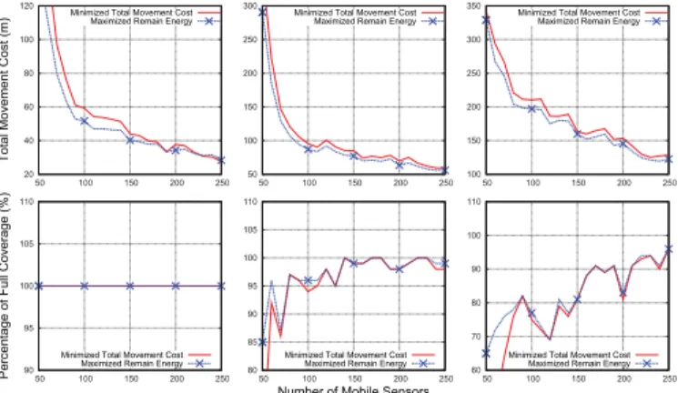
To evaluate the efficiency of our proposed optimization function, we compare it to the current best solution suggested for hybrid sensor networks [2]. The testbed is set up as follows: we consider a network deployed in an area of different sizes 100m×100m, 200m×200m and400m×400m. All networks contain 20 randomly located coverage holes. We randomly deploy various numbers mobile sensors, each sensor of which is uniformly initialized a random amount of energy ranging from 2500J to3000J. We allow each mobile sensor to consume about 30J per meter [7].
In each configuration of the area size and mobile sensors, we move mobile sensors according to two optimal schedules (1) Maximizing the minimum remaining energy (Ours) and (2) Minimizing the total movement distance (Wang’s [2]). By the time the sensors with minimum energy in [2] run out of energy, we again execute Wang’s method to heal all holes created by these sensors.
As depicted in Fig. 4, our approach most of the time produces very competitive, if not to say better, results in comparison with the current best method. In particular, our total movement costs are always lower than those of Wang’s in all test cases (top figures), except for some unusual cases where the density of mobile sensors is extremely high (e.g., when number of sensors is 300 in the top left figure). In particular, our results are around 3% to 9% better than that of Wang’s. These results confirm the utilization strength of our proposed metric.
Competitions on the network coverage (Fig. 4) reveal that our algorithm, again, achieves competitive coverage percent-age with its competitor, especially in the first test case where both cover 100% of the network (left down figure). In the other test cases, our method is a little bit off when the number of sensors is small (e.g., less than 60 sensors); however, in a long run, ours is better than Wang’s method with 2% to 5% and 2% to 3% more of the target field covered as shown in middle and right down figures, respectively. One of the key reasons is that in Wang’s method, mobile sensors are moved regardless of their remaining energy, thereby increasing the posiblity of re-executing the movement schedule more frequently. It implies that during the re-execution, coverage holes are left unhealed. Supported by these experimental results, we believe that our new optimization metric is more efficient and robust in comparison to the current best one proposed in [2].
20 40 60 80 100 120 50 100 150 200 250
Total Movement Cost (m)
Minimized Total Movement Cost Maximized Remain Energy
50 100 150 200 250 300 50 100 150 200 250
Minimized Total Movement Cost Maximized Remain Energy
100 150 200 250 300 350 50 100 150 200 250
Minimized Total Movement Cost Maximized Remain Energy
90 95 100 105 110 50 100 150 200 250
Percentage of Full Coverage (%)
Minimized Total Movement Cost Maximized Remain Energy
80 85 90 95 100 105 110 50 100 150 200 250 Number of Mobile Sensors
Minimized Total Movement Cost Maximized Remain Energy
60 70 80 90 100 110 50 100 150 200 250
Minimized Total Movement Cost Maximized Remain Energy
Fig. 4. Two optimal movement schedules with different objectives: max-imized minimum remained energy and minmax-imized total movement cost. Two left figures are of size 100m×100m. Middle figures are of size
200m×200m. Two right figures are of size400m×400m.
B. The advantage of cascaded movement
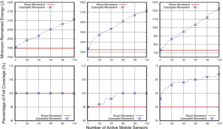
We use the same testbed as above with the appearance of coverage holes. Each network contains 20 randomly located coverage holes and 50 randomly placed inactive mobile sen-sors. To allow the cascaded movement, we also deploy active mobile sensors which are randomly assigned ranging from 1500J to 3000J [7]. We run 100 times and compute the average of the lowest remained energy overall moved sensors with two options: with and without cascaded movement.
The dominance of mobile sensor scheduling with over without cascaded movement is shown in Fig. 5. As indicated in this figure, the allowance of cascaded movement significantly helps the mobile sensors to attain much more remaining energy, especially when the number of sensors increases. In particular, a scheduling with cascaded movement helps sensors save up to 7%, 21% and 71% more energy in the hole healing process, as depicted in the top left, top middle and top right figure, respectively. The reason behind this superiority is due to the lesser distance each sensors has to travel in order to heal a coverage hole. These results promise the advantage of a scheduling with cascaded movement in a hybrid sensor network.
Experiments on network coverage, again, confirm the ef-fectiveness of a scheduling with cascaded movement. As one can observe from the results depicted in the left, middle and right down figures, the percentage of the targeting area covered by mobile sensors with cascaded movements increases signif-icantly and tends to double that of non-cascaded movement when the number of deployed sensor increases. These results prove the strength of our proposed algorithm with cascaded movement.
C. The efficiency of the distributed scheme
Finally, we test the distributed scheme when the network has only one coverage hole and compare the results with the optimal solutions. We use the same set up as above with a slight modification: the size of a cell is 10m×10m, which implies a 400m×400m-field will have 1600 cells. A set of mobile sensors are randomly located in the field of target. We
1900 1950 2000 2050 2100 2150 2200 0 20 40 60 80 100
Minimum Remained Energy (J)
Direct Movement Cascaded Movement 1300 1400 1500 1600 1700 1800 0 20 40 60 80 100 Direct Movement Cascaded Movement 700 800 900 1000 1100 1200 1300 0 20 40 60 80 100 Direct Movement Cascaded Movement 90 95 100 105 110 0 20 40 60 80 100
Percentage of Full Coverage (%)
Direct Movement Cascaded Movement 90 95 100 105 110 0 20 40 60 80 100 Number of Active Mobile Sensors
Direct Movement Cascaded Movement 50 55 60 65 70 0 20 40 60 80 100 Direct Movement Cascaded Movement
Fig. 5. Minimum remained energy of moved sensors in cascaded movement and direct movement. Two left figures are of size 100m×100m. Middle figures are of size200m×200m. Two right figures are of size400m×400m.
2300 2400 2500 2600 2700 2800 2900 3000 50 100 150 200 250 Remained Energy (J)
Optimal Remained Energy Distributed Scheme 2300 2400 2500 2600 2700 2800 2900 3000 50 100 150 200 250 Number of Mobile Sensors
Optimal Remained Energy Distributed Scheme 2300 2400 2500 2600 2700 2800 2900 3000 50 100 150 200 250
Optimal Remained Energy Distributed Scheme
Fig. 6. The near optimality of the Distributed Scheme. Left figure is of size
100m×100m. Middle figure is of size200m×200m. Right figure is of size400m∗400m.
generate 100 networks, each of them contains 1000 coverage holes randomly deployed in the targeting area.
As shown in Fig. 6, the energy differences between the our heuristic results and the optimal solutions are quite small: the remaining energy of our distributed algorithm covers up to 95%, 96% and 98% of the energy produced by the optimal so-lution. Moreover, our results tend to closely approximate those of the optimal methods as the number of sensors increases. This result indicates that when only a small number of holes develops, our distributed algorithm efficiently computes a scheduling that relatively preserves as much remaining energy as the optimal strategy does.
VI. RELATEDWORK
On hybrid sensor networks, Wang et al.[8] proposed a bidding protocol between static and mobile sensors to guide the movement of mobile sensors. Static sensors detect the coverage holes and then send bidding messages to mobile ones. After several rounds of exchanging information, a mobile sensor moves to the nearest matched hole. This protocol is time consuming and computationally expensive. In another work [2], Wang et al. designed an optimal algorithm to move mobile sensors such that the total movement distance is minimized. However, this approach has the limitation as we discussed in Section I, which gives rise to our metric. Using a somehow similar metric with ours, Czyzowicz et al. [9] proposed an O(n2)optimal algorithm that maps mobile sensors in a line segment. Because in the line segment, mobile sensors can only choose two directions to move, the solution is not extended to wireless sensor networks that monitor a square area.
Instead of healing several coverage holes simultaneously, there exists some studies focused on healing one single hole [10], [11], [12] (and references therein). The notable common limitations of these methods are two fold: 1) high message and computational complexity and 2) it is not easy to extend these solutions for multiple coverage holes healing as addressed in our paper.
VII. CONCLUSION
In this paper, we study the coverage healing problem with the different metric on hybrid sensor networks where both static and mobile sensors are utilized. We proposed a new metric to maximize the minimum remaining energy over all moved sensors. Based on this new metric, we proposed a graph theory based approach for the coverage healing problem which always returns an optimal solution according to this metric. We also presented a near-optimal distributed algorithm for a special case when the number of newly introduced coverage holes is small. Experimental results show that our new metric helps the WSN work much more stabler and last longer in comparison to the total consumed energy metric in [2].
ACKNOWLEDGMENT
This work is partially supported by NSF CAREER 0953284 and DTRA HDTRA1-08-10.
REFERENCES
[1] N. Xu. A survey of sensor network applications.IEEE Communications Magazine, 40(8):102–114, 2002.
[2] Wei Wang, Vikram Srinivasan, and Kee-Chaing Chua. Trade-offs between mobility and density for coverage in wireless sensor networks.
MOBICOM, pages 39–50, 2007.
[3] R.A.F. Mini, M. Val Machado, A.A.F. Loureiro, and B. Nath. Prediction-based energy map for wireless sensor networks. Ad Hoc Networks, 3(2):235–253, 2005.
[4] N. Bulusu, J. Heidemann, and D. Estrin. Gps-less low-cost outdoor localization for very small devices. Personal Communications, IEEE, 7(5):28 –34, October 2000.
[5] Amitabha Ghosh. Estimating coverage holes and enhancing coverage in mixed sensor networks. In Proceedings of the 29th Annual IEEE International Conference on Local Computer Networks, LCN ’04, pages 68–76, Washington, DC, USA, 2004. IEEE Computer Society. [6] John E. Hopcroft and Richard M. Karp. A n5/2 algorithm for maximum
matchings in bipartite. InSwitching and Automata Theory, 1971., 12th Annual Symposium on, pages 122 –125, oct. 1971.
[7] Gabe Sibley and Mohammad H. Rahimi andGaurav S. Sukhatme. Robomote: A tiny mobile robot platform for large-scale ad-hoc sensor networks. InICRA, pages 1143–1148, 2002.
[8] Guiling Wang, Guohong Cao, and T. LaPorta. A bidding protocol for deploying mobile sensors. In Network Protocols, 2003. Proceedings. 11th IEEE International Conference on, pages 315 – 324, 2003. [9] J. Czyzowicz, E. Kranakis, D. Krizanc, I. Lambadaris, L. Narayanan,
J. Opatrny, L. Stacho, J. Urrutia, and M. Yazdani. On minimizing the maximum sensor movement for barrier coverage of a line segment. In
ADHOC-NOW ’09: Proceedings of the 8th International Conference on Ad-Hoc, Mobile and Wireless Networks, pages 194–212. Springer-Verlag, 2009.
[10] Guiling Wang, Guohong Cao, T. La Porta, and Wensheng Zhang. Sensor relocation in mobile sensor networks. InINFOCOM 2005. 24th Annual Joint Conference of the IEEE Computer and Communications Societies. Proceedings IEEE, volume 4, pages 2302 –2312 vol. 4, march 2005. [11] Xu Li, Nicola Santoro, and Ivan Stojmenovic. Mesh-based sensor
relocation for coverage maintenance in mobile sensor networks. In
Ubiquitous Intelligence and Computing, Lecture Notes in Computer Science. Springer Berlin / Heidelberg, 2007.
[12] Xu Li and N. Santoro. Zoner: A zone-based sensor relocation protocol for mobile sensor networks. Local Computer Networks, Proceedings 2006 31st IEEE Conference on, 2006.