The Isabelle/Isar Reference Manual

λ → ∀ =

Isabelle

The Isabelle/Isar Reference Manual

Makarius Wenzel

With Contributions by Clemens Ballarin, Stefan Berghofer,

Jasmin Blanchette, Timothy Bourke, Lukas Bulwahn,

Amine Chaieb, Lucas Dixon, Florian Haftmann,

Brian Huffman, Lars Hupel, Gerwin Klein,

Alexander Krauss, Ondřej Kunčar, Andreas Lochbihler,

Tobias Nipkow, Lars Noschinski, David von Oheimb,

Larry Paulson, Sebastian Skalberg, Christian Sternagel

The Isabelle system essentially provides a generic infrastructure for building deductive systems (programmed in Standard ML), with a special focus on interactive theorem proving in higher-order logics. Many years ago, even end-users would refer to certain ML functions (goal commands, tactics, tacticals etc.) to pursue their everyday theorem proving tasks.

In contrast Isar provides an interpreted language environment of its own, which has been specifically tailored for the needs of theory and proof devel-opment. Compared to raw ML, the Isabelle/Isar top-level provides a more robust and comfortable development platform, with proper support for the-ory development graphs, managed transactions with unlimited undo etc. In its pioneering times, the Isabelle/Isar version of theProof General user in-terface [2, 3] has contributed to the success of for interactive theory and proof development in this advanced theorem proving environment, even though it was somewhat biased towards old-style proof scripts. The more recent Isabelle/jEdit Prover IDE [56] emphasizes the document-oriented approach of Isabelle/Isar again more explicitly.

Apart from the technical advances over bare-bones ML programming, the main purpose of the Isar language is to provide a conceptually different view on machine-checked proofs [53, 54]. Isar stands for Intelligible semi-automated reasoning. Drawing from both the traditions of informal mathe-matical proof texts and high-level programming languages, Isar offers a ver-satile environment for structured formal proof documents. Thus properly written Isar proofs become accessible to a broader audience than unstruc-tured tactic scripts (which typically only provide operational information for the machine). Writing human-readable proof texts certainly requires some additional efforts by the writer to achieve a good presentation, both of formal and informal parts of the text. On the other hand, human-readable formal texts gain some value in their own right, independently of the mechanic proof-checking process.

Despite its grand design of structured proof texts, Isar is able to assimilate the old tactical style as an “improper” sub-language. This provides an easy upgrade path for existing tactic scripts, as well as some means for interactive experimentation and debugging of structured proofs. Isabelle/Isar supports

a broad range of proof styles, both readable and unreadable ones.

The generic Isabelle/Isar framework (see chapter 2) works reasonably well for any Isabelle object-logic that conforms to the natural deduction view of the Isabelle/Pure framework. Specific language elements introduced by Isabelle/HOL are described in part III. Although the main language elements are already provided by the Isabelle/Pure framework, examples given in the generic parts will usually refer to Isabelle/HOL.

Isar commands may be either proper document constructors, or improper

commands. Some proof methods and attributes introduced later are classified as improper as well. Improper Isar language elements, which are marked by “∗_{” in the subsequent chapters; they are often helpful when developing}

proof documents, but their use is discouraged for the final human-readable outcome. Typical examples are diagnostic commands that print terms or theorems according to the current context; other commands emulate old-style tactical theorem proving.

I

Basic Concepts

1

1 Synopsis 2

1.1 Notepad . . . 2

1.1.1 Types and terms . . . 2

1.1.2 Facts . . . 2

1.1.3 Block structure . . . 5

1.2 Calculational reasoning . . . 6

1.2.1 Special names in Isar proofs . . . 6

1.2.2 Transitive chains . . . 7

1.2.3 Degenerate calculations and bigstep reasoning . . . 8

1.3 Induction . . . 9

1.3.1 Induction as Natural Deduction . . . 9

1.3.2 Induction with local parameters and premises . . . 11

1.3.3 Implicit induction context . . . 12

1.3.4 Advanced induction with term definitions . . . 13

1.4 Natural Deduction . . . 13

1.4.1 Rule statements . . . 13

1.4.2 Isar context elements . . . 15

1.4.3 Pure rule composition . . . 16

1.4.4 Structured backward reasoning . . . 16

1.4.5 Structured rule application . . . 17

1.4.6 Example: predicate logic . . . 18

1.5 Generalized elimination and cases . . . 22

1.5.1 General elimination rules . . . 22

1.5.2 Rules with cases . . . 23

1.5.3 Obtaining local contexts . . . 24

2 The Isabelle/Isar Framework 25

2.1 The Pure framework . . . 27

2.1.1 Primitive inferences . . . 28

2.1.2 Reasoning with rules . . . 29

2.2 The Isar proof language . . . 31

2.2.1 Context elements . . . 32

2.2.2 Structured statements . . . 34

2.2.3 Structured proof refinement . . . 35

2.2.4 Calculational reasoning . . . 37

2.3 Example: First-Order Logic . . . 38

2.3.1 Equational reasoning . . . 39

2.3.2 Basic group theory . . . 40

2.3.3 Propositional logic . . . 41

2.3.4 Classical logic . . . 43

2.3.5 Quantifiers . . . 44

2.3.6 Canonical reasoning patterns . . . 45

II

General Language Elements

48

3.2 Lexical matters . . . 50

3.3 Common syntax entities . . . 52

3.3.1 Names . . . 52

3.3.2 Numbers . . . 53

3.3.3 Comments . . . 54

3.3.4 Type classes, sorts and arities . . . 54

3.3.5 Types and terms . . . 55

3.3.6 Term patterns and declarations . . . 57

3.3.7 Attributes and theorems . . . 59

4 Document preparation 63 4.1 Markup commands . . . 63

4.2 Document antiquotations . . . 65

4.2.1 Styled antiquotations . . . 71

4.3 Markup via command tags . . . 73

4.4 Railroad diagrams . . . 74

4.5 Draft presentation . . . 78

5 Specifications 79 5.1 Defining theories . . . 79

5.2 Local theory targets . . . 82

5.3 Bundled declarations . . . 84 5.4 Term definitions . . . 85 5.5 Axiomatizations . . . 87 5.6 Generic declarations . . . 88 5.7 Locales . . . 89 5.7.1 Locale expressions . . . 89 5.7.2 Locale declarations . . . 91 5.7.3 Locale interpretation . . . 94 5.8 Classes . . . 100

5.8.1 The class target . . . 103

5.8.2 Co-regularity of type classes and arities . . . 103

5.9 Unrestricted overloading . . . 104

5.10 Incorporating ML code . . . 105

5.11 Primitive specification elements . . . 107

5.11.1 Sorts . . . 107

5.11.2 Types . . . 108

5.11.3 Constants and definitions . . . 109

5.12 Naming existing theorems . . . 110

5.13 Oracles . . . 111 5.14 Name spaces . . . 112 6 Proofs 113 6.1 Proof structure . . . 113 6.1.1 Formal notepad . . . 113 6.1.2 Blocks . . . 114 6.1.3 Omitting proofs . . . 115 6.2 Statements . . . 115 6.2.1 Context elements . . . 115

6.2.2 Term abbreviations . . . 117

6.2.3 Facts and forward chaining . . . 118

6.2.4 Goals . . . 120

6.3 Refinement steps . . . 123

6.3.1 Proof method expressions . . . 123

6.3.2 Initial and terminal proof steps . . . 125

6.3.3 Fundamental methods and attributes . . . 127

6.3.4 Emulating tactic scripts . . . 130

6.3.5 Defining proof methods . . . 132

6.4 Generalized elimination . . . 133

6.5 Calculational reasoning . . . 134

6.6 Proof by cases and induction . . . 136

6.6.1 Rule contexts . . . 136

6.6.2 Proof methods . . . 139

6.6.3 Declaring rules . . . 145

7 Inner syntax — the term language 146 7.1 Printing logical entities . . . 146

7.1.1 Diagnostic commands . . . 146

7.1.2 Details of printed content . . . 149

7.1.3 Alternative print modes . . . 151

7.2 Mixfix annotations . . . 152

7.2.1 The general mixfix form . . . 153

7.2.2 Infixes . . . 154

7.2.3 Binders . . . 155

7.3 Explicit notation . . . 156

7.4 The Pure syntax . . . 157

7.4.1 Lexical matters . . . 157

7.4.2 Priority grammars . . . 158

7.4.3 The Pure grammar . . . 159

7.4.4 Inspecting the syntax . . . 163

7.4.5 Ambiguity of parsed expressions . . . 164

7.5 Syntax transformations . . . 165

7.5.1 Abstract syntax trees . . . 166

7.5.3 Syntax translation functions . . . 173

7.5.4 Built-in syntax transformations . . . 175

8 Other commands 179 8.1 Inspecting the context . . . 179

9 Generic tools and packages 183 9.1 Configuration options . . . 183

9.2 Basic proof tools . . . 184

9.2.1 Miscellaneous methods and attributes . . . 184

9.2.2 Low-level equational reasoning . . . 187

9.2.3 Further tactic emulations . . . 188

9.3 The Simplifier . . . 192

9.3.1 Simplification methods . . . 192

9.3.2 Declaring rules . . . 197

9.3.3 Ordered rewriting with permutative rules . . . 200

9.3.4 Simplifier tracing and debugging . . . 202

9.3.5 Simplification procedures . . . 203

9.3.6 Configurable Simplifier strategies . . . 205

9.3.7 Forward simplification . . . 209

9.4 The Classical Reasoner . . . 210

9.4.1 Basic concepts . . . 210

9.4.2 Rule declarations . . . 214

9.4.3 Structured methods . . . 216

9.4.4 Fully automated methods . . . 217

9.4.5 Partially automated methods . . . 221

9.4.6 Single-step tactics . . . 222

9.4.7 Modifying the search step . . . 223

9.5 Object-logic setup . . . 224

9.6 Tracing higher-order unification . . . 226

III

Isabelle/HOL

227

11 Derived specification elements 230

11.1 Inductive and coinductive definitions . . . 230

11.1.1 Derived rules . . . 232

11.1.2 Monotonicity theorems . . . 233

11.2 Recursive functions . . . 234

11.2.1 Proof methods related to recursive definitions . . . 239

11.2.2 Functions with explicit partiality . . . 241

11.2.3 Old-style recursive function definitions (TFL) . . . 242

11.3 Old-style datatypes . . . 244

11.4 Records . . . 246

11.4.1 Basic concepts . . . 246

11.4.2 Record specifications . . . 247

11.4.3 Record operations . . . 248

11.4.4 Derived rules and proof tools . . . 249

11.5 Typedef axiomatization . . . 250

11.6 Functorial structure of types . . . 253

11.7 Quotient types . . . 254

11.8 Definition by specification . . . 257

11.9 Adhoc overloading of constants . . . 258

12 Proof tools 260 12.1 Adhoc tuples . . . 260

12.2 Transfer package . . . 260

12.3 Lifting package . . . 262

12.4 Coercive subtyping . . . 268

12.5 Arithmetic proof support . . . 269

12.6 Intuitionistic proof search . . . 269

12.7 Model Elimination and Resolution . . . 270

12.8 Algebraic reasoning via Gröbner bases . . . 270

12.9 Coherent Logic . . . 272

12.10Proving propositions . . . 272

12.11Checking and refuting propositions . . . 274

12.12Unstructured case analysis and induction . . . 279

IV

Appendix

293

A Isabelle/Isar quick reference 294

A.1 Proof commands . . . 294

A.1.1 Primitives and basic syntax . . . 294

A.1.2 Abbreviations and synonyms . . . 295

A.1.3 Derived elements . . . 295

A.1.4 Diagnostic commands . . . 295

A.2 Proof methods . . . 296

A.3 Attributes . . . 297

A.4 Rule declarations and methods . . . 297

A.5 Emulating tactic scripts . . . 298

A.5.1 Commands . . . 298

A.5.2 Methods . . . 298

B Predefined Isabelle symbols 299 C ML tactic expressions 305 C.1 Resolution tactics . . . 305

C.2 Simplifier tactics . . . 306

C.3 Classical Reasoner tactics . . . 306

C.4 Miscellaneous tactics . . . 307

C.5 Tacticals . . . 307

Bibliography 308

Basic Concepts

Synopsis

1.1

Notepad

An Isar proof body serves as mathematical notepad to compose logical con-tent, consisting of types, terms, facts.

1.1.1

Types and terms

begin

Locally fixed entities:

fix x — local constant, without any type information yet

fix x :: 0a — variant with explicit type-constraint for subsequent use

fix a b

assume a = b — type assignment at first occurrence in concrete term

Definitions (non-polymorphic): defx ≡t::0a Abbreviations (polymorphic): let ?f = λx.x term ?f ?f Notation: write x (∗∗∗) end

1.1.2

Facts

A fact is a simultaneous list of theorems.

Producing facts notepad

begin

Via assumption (“lambda”): assume a:A

Via proof (“let”): have b:B sorry Via abbreviation (“let”):

notec =a b

end

Referencing facts notepad

begin

Via explicit name: assume a:A

notea

Via implicit name: assume A

notethis

Via literal proposition (unification with results from the proof text): assume A notehAi assume V x. B x noteh_{B a}i notehB bi end Manipulating facts notepad begin Instantiation:

assume a:V x.B x notea notea [of b] notea [where x =b] Backchaining: assume 1: A assume 2: A =⇒ C note2 [OF 1] note1 [THEN 2] Symmetric results: assume x = y

notethis [symmetric] assume x 6= y

notethis [symmetric]

Adhoc-simplification (take care!): assume P ([] @xs)

notethis [simplified] end

Projections

Isar facts consist of multiple theorems. There is notation to project interval ranges. notepad begin assume stuff: A B C D notestuff(1) notestuff(2−3) notestuff(2−) end Naming conventions

• Lower-case identifiers are usually preferred.

• Facts can be named after the main term within the proposition.

• Facts should not be named after the command that introduced them

• Natural numbers can be used as “meaningless” names (more appropri-ate than a1,a2etc.)

• Symbolic identifiers are supported (e.g. ∗, ∗∗,∗∗∗).

1.1.3

Block structure

The formal notepad is block structured. The fact produced by the last entry of a block is exported into the outer context.

notepad begin { havea:A sorry haveb:B sorry notea b } notethis noteh_Ai notehBi end

Explicit blocks as well as implicit blocks of nested goal statements (e.g.have) automatically introduce one extra pair of parentheses in reserve. The next command allows to “jump” between these sub-blocks.

notepad begin { havea:A sorry next haveb:B proof − show B sorry next have c: C sorry next have d:D sorry qed }

{ { have a: A sorry } { have b: B proof − { show B sorry } { have c: C sorry } { have d:D sorry } qed } } end

1.2

Calculational reasoning

For example, see ~~/src/HOL/Isar_Examples/Group.thy.

1.2.1

Special names in Isar proofs

• term?thesis — the main conclusion of the innermost pending claim • term . . . — the argument of the last explicitly stated result (for infix

application this is the right-hand side)

• fact this — the last result produced in the text

notepad begin

have x =y

proof −

term?thesis

show?thesis sorry term?thesis — static!

qed term . . .

thm this

end

Calculational reasoning maintains the special fact called “calculation” in the background. Certain language elements combine primarythis with secondary calculation.

1.2.2

Transitive chains

The Idea is to combine this and calculation via typical trans rules (see also print_trans_rules): thm trans thm less_trans thm less_le_trans notepad begin

Plain bottom-up calculation: have a =b sorry also have b =c sorry also have c =d sorry finally have a =d .

Variant using the . . . abbreviation:

have a =b sorry also have . . . =c sorry also have . . . =d sorry finally have a =d .

Top-down version with explicit claim at the head: have a =d

proof −

also have. . . = c sorry also have. . . = d sorry finally show?thesis . qed next

Mixed inequalities (require suitable base type): fix a b c d :: nat have a <b sorry also have b ≤c sorry also have c =d sorry finally have a <d . end Notes

• The notion of trans rule is very general due to the flexibility of

Isabelle/Pure rule composition.

• User applications may declare their own rules, with some care about the operational details of higher-order unification.

1.2.3

Degenerate calculations and bigstep reasoning

notepad begin A vacuous proof: have Asorry moreover have B sorry moreover have C sorry

ultimately

have Aand B and C . next

Slightly more content (trivial bigstep reasoning): have Asorry moreover have B sorry moreover have C sorry ultimately have A∧ B ∧ C byblast next

More ambitious bigstep reasoning involving structured results: have A∨ B ∨ C sorry

moreover

{ assumeA have R sorry } moreover

{ assumeB have R sorry } moreover

{ assumeC have R sorry } ultimately

have Rby blast — “big-bang integration” of proof blocks (occasionally fragile)

end

1.3

Induction

1.3.1

Induction as Natural Deduction

In principle, induction is just a special case of Natural Deduction (see also §1.4). For example:

thm nat.induct

print_statement nat.induct

notepad begin

fix n :: nat

have P n

proof (rule nat.induct) — fragile rule application! showP 0 sorry

fix n :: nat

assume P n

showP (Suc n) sorry qed

end

In practice, much more proof infrastructure is required. The proof method induct provides:

• implicit rule selection and robust instantiation • context elements via symbolic case names

• support for rule-structured induction statements, with local parame-ters, premises, etc.

notepad begin fix n :: nat have P n proof (induct n) case 0

show?case sorry next

case (Suc n)

from Suc.hyps show ?case sorry qed

end Example

The subsequent example combines the following proof patterns:

• outermost induction (over the datatype structure of natural numbers), to decompose the proof problem in top-down manner

• calculational reasoning (§1.2) to compose the result in each case • solving local claims within the calculation by simplification

lemma

fixes n :: nat

shows (P

i=0..n.i) =n ∗ (n + 1) div 2 proof (induct n)

case 0 have (P

i=0..0.i) = (0::nat) bysimp

also have. . . = 0 ∗ (0 + 1) div 2 by simp

finally show ?case . next

case (Suc n) have (P

i=0..Suc n.i) = (P

i=0..n.i) + (n + 1) by simp

also have. . . = n ∗ (n + 1)div 2 + (n + 1) by (simp add: Suc.hyps) also have. . . = (n ∗ (n + 1) + 2∗ (n + 1)) div 2 by simp

also have. . . = (Suc n ∗ (Suc n + 1)) div 2 bysimp

finally show ?case . qed

This demonstrates how induction proofs can be done without having to con-sider the raw Natural Deduction structure.

1.3.2

Induction with local parameters and premises

Important: Using compact HOL formulae with ∀/−→ is a well-known

anti-pattern! It would produce useless formal noise.

notepad begin

fix n :: nat

fix P ::nat ⇒ bool

fix Q :: 0a ⇒ nat ⇒ bool

have P n proof (induct n) case 0 showP 0 sorry next case (Suc n)

from hP ni show P (Suc n) sorry qed

have A n =⇒ P n

proof (induct n) case 0

next

case (Suc n)

from hA n =⇒ P ni

and h_{A (Suc n)}i_{show P (Suc n) sorry} qed have V x.Q x n proof (induct n) case 0 showQ x 0 sorry next case (Suc n)

from hV_{x. Q x n}i_{show Q x (Suc n) sorry} Local quantification admits arbitrary instances:

notehQ a ni andhQ b ni qed

end

1.3.3

Implicit induction context

The induct method can isolate local parameters and premises directly from the given statement. This is convenient in practical applications, but requires some understanding of what is going on internally (as explained above).

notepad begin

fix n :: nat

fix Q :: 0a ⇒ nat ⇒ bool

fix x :: 0a

assume A x n

then have Q x n

proof (induct n arbitrary:x) case 0

from h_{A x} 0i_{show Q x} 0 _sorry next

case (Suc n)

from hV_x. _{A x n} =⇒ _{Q x n}i — arbitrary instances can be produced here and h_{A x (Suc n)}i_{show Q x (Suc n) sorry}

qed end

1.3.4

Advanced induction with term definitions

Induction over subexpressions of a certain shape are delicate to formalize. The Isar induct method provides infrastructure for this.

Idea: sub-expressions of the problem are turned into a defined induction variable; often accompanied with fixing of auxiliary parameters in the original expression.

notepad begin

fix a :: 0a ⇒ nat

fix A :: nat ⇒ bool

assume A (a x) then have P (a x)

proof (induct a x arbitrary: x) case 0 noteprem = h_{A (a x)}i and defn =h_{0 =a x}i showP (a x) sorry next case (Suc n) notehyp = hVx. n =a x =⇒ A (a x) =⇒ P (a x)i and prem =h_{A (a x)}i

and defn =h_{Suc n = a x}i showP (a x) sorry

qed end

1.4

Natural Deduction

1.4.1

Rule statements

Isabelle/Pure “theorems” are always natural deduction rules, which some-times happen to consist of a conclusion only.

The framework connectives V and

=⇒ indicate the rule structure declara-tively. For example:

thm conjI

thm impI

thm nat.induct

The object-logic is embedded into the Pure framework via an implicit deriv-ability judgment Trueprop :: bool ⇒ prop.

Thus any HOL formulae appears atomic to the Pure framework, while the rule structure outlines the corresponding proof pattern.

This can be made explicit as follows:

notepad begin write Trueprop (Tr) thm conjI thm impI thm nat.induct end

Isar provides first-class notation for rule statements as follows.

print_statement conjI

print_statement impI

print_statement nat.induct

Examples

Introductions and eliminations of some standard connectives of the object-logic can be written as rule statements as follows. (The proof “by blast” serves as sanity check.)

lemma (P =⇒ False) =⇒ ¬ P byblast

lemma ¬ P =⇒ P =⇒ Q by blast lemma P =⇒ Q =⇒ P ∧ Q byblast lemma P ∧Q =⇒ (P =⇒ Q =⇒ R) =⇒ R by blast lemma P =⇒ P ∨ Q byblast lemma Q =⇒ P ∨Q by blast lemma P ∨Q =⇒ (P =⇒ R) =⇒ (Q =⇒ R) =⇒ R byblast lemma (V x.P x) =⇒ (∀x.P x) byblast lemma (∀x.P x) =⇒ P x byblast lemma P x =⇒ (∃x.P x) byblast lemma (∃x.P x) =⇒ (V x.P x =⇒ R) =⇒ R byblast lemma x ∈ A =⇒ x ∈ B =⇒ x ∈ A ∩ B byblast lemma x ∈ A ∩ B =⇒ (x ∈ A =⇒ x ∈ B =⇒ R) =⇒ R by blast lemma x ∈ A =⇒ x ∈ A ∪ B byblast

lemma x ∈ B =⇒ x ∈ A ∪ B byblast

lemma x ∈ A ∪ B =⇒ (x ∈ A =⇒ R) =⇒ (x ∈B =⇒ R) =⇒ R byblast

1.4.2

Isar context elements

We derive some results out of the blue, using Isar context elements and some explicit blocks. This illustrates their meaning wrt. Pure connectives, without goal states getting in the way.

notepad begin { fix x haveB x sorry } have V x.B x byfact next { assume A haveB sorry } have A=⇒ B byfact next { defx ≡ t haveB x sorry } have B t byfact next {

obtainx :: 0a whereB x sorry haveC sorry

}

have C by fact

1.4.3

Pure rule composition

• backward-chaining of rules by resolution • closing of branches by assumption

Both principles involve higher-order unification of λ-terms modulo αβη

-equivalence (cf. Huet and Miller).

notepad begin

assume a:A and b:B

thm conjI

thm conjI [of A B] — instantiation

thm conjI [of A B, OF a b] — instantiation and composition thm conjI [OF a b] — composition via unification (trivial) thm conjI [OF h_Ai h_Bi_]

thm conjI [OF disjI1] end

Note: Low-level rule composition is tedious and leads to unreadable / un-maintainable expressions in the text.

1.4.4

Structured backward reasoning

Idea: Canonical proof decomposition via fix / assume / show, where the

body produces a natural deduction rule to refine some goal.

notepad begin fix A B :: 0a ⇒ bool have V x.A x =⇒ B x proof − fix x assume A x showB x sorry qed have V x.A x =⇒ B x proof −

{ fix x

assume A x

show B x sorry

} — implicit block structure made explicit notehVx.A x =⇒ B xi

— side exit for the resulting rule qed

end

1.4.5

Structured rule application

Idea: Previous facts and new claims are composed with a rule from the con-text (or background library).

notepad begin

assume r1:A =⇒ B =⇒ C — simple rule (Horn clause)

have Asorry — prefix of facts via outer sub-proof then have C

proof (rule r1)

showB sorry — remaining rule premises via inner sub-proof qed have C proof (rule r1) showA sorry showB sorry qed

have Aand B sorry then have C

proof (rule r1) qed

have Aand B sorry then have C by (rule r1) next

assume r2:A =⇒ (V

x.B1 x =⇒ B2 x) =⇒ C — nested rule

then have C proof (rule r2) fix x assume B1 x showB2 x sorry qed

The compound rule premise V

x. B1 x =⇒ B2 x is better addressed via fix / assume / showin the nested proof body.

end

1.4.6

Example: predicate logic

Using the above principles, standard introduction and elimination proofs of predicate logic connectives of HOL work as follows.

notepad begin

have A−→ B andA sorry then have B .. have Asorry then have A ∨ B .. have B sorry then have A ∨ B .. have A∨ B sorry then have C proof assume A

then show C sorry next

assume B

then show C sorry qed

have Aand B sorry then have A ∧ B .. have A∧ B sorry then have A .. have A∧ B sorry

then have B .. have False sorry then have A .. have True .. have ¬A

proof assume A

then show False sorry qed

have ¬A and A sorry then have B .. have ∀x.P x proof fix x showP x sorry qed have ∀x.P x sorry then have P a .. have ∃x.P x proof showP a sorry qed have ∃x.P x sorry then have C proof fix a assume P a showC sorry qed

Less awkward version using obtain: have ∃x.P x sorry

then obtain a where P a .. end

notepad begin

have A∧ B

proof — two strictly isolated subproofs showA sorry

next

showB sorry qed

have A∧ B

proof — one simultaneous sub-proof showA and B sorry

qed

have A∧ B

proof — two subproofs in the same context showA sorry

showB sorry qed

have A∧ B

proof — swapped order showB sorry

showA sorry qed

have A∧ B

proof — sequential subproofs showA sorry

showB using hAisorry qed

end

Example: set-theoretic operators

There is nothing special about logical connectives (∧, ∨,∀, ∃ etc.). Opera-tors from set-theory or lattice-theory work analogously. It is only a matter of rule declarations in the library; rules can be also specified explicitly.

notepad begin

have x ∈ Aand x ∈ B sorry then have x ∈ A ∩ B ..

have x ∈ Asorry then have x ∈ A ∪ B .. have x ∈ B sorry then have x ∈ A ∪ B .. have x ∈ A∪ B sorry then have C proof assume x ∈ A

then show C sorry next

assume x ∈ B

then show C sorry qed next have x ∈ T A proof fix a assume a ∈ A showx ∈a sorry qed have x ∈ T A sorry then have x ∈ a proof showa ∈ Asorry qed

have a ∈ A andx ∈ a sorry then have x ∈ S

A .. have x ∈ S

A sorry

then obtain a where a ∈ A andx ∈ a .. end

1.5

Generalized elimination and cases

1.5.1

General elimination rules

The general format of elimination rules is illustrated by the following typical representatives:

thm exE — local parameter

thm conjE — local premises

thm disjE — split into cases

Combining these characteristics leads to the following general scheme for elimination rules with cases:

• prefix of assumptions (or “major premises”)

• one or more cases that enable to establish the main conclusion in an augmented context notepad begin assume r: A1 =⇒ A2 =⇒ (∗ assumptions ∗) (V x y.B1 x y =⇒ C1 x y =⇒ R) =⇒ (∗ case 1 ∗) (V x y.B2 x y =⇒ C2 x y =⇒ R) =⇒ (∗ case 2 ∗) R (∗ main conclusion ∗) have A1 andA2 sorry then have R

proof (rule r) fix x y

assume B1 x y and C1 x y

show?thesis sorry next

fix x y

assume B2 x y and C2 x y

show?thesis sorry qed

end

1.5.2

Rules with cases

Applying an elimination rule to some goal, leaves that unchanged but allows to augment the context in the sub-proof of each case.

Isar provides some infrastructure to support this: • native language elements to state eliminations • symbolic case names

• methodcases to recover this structure in a sub-proof

print_statement exE

print_statement conjE

print_statement disjE

lemma

assumesA1 andA2 — assumptions obtains

(case1) x y whereB1 x y andC1 x y

|(case2) x y whereB2 x y and C2 x y

sorry Example lemma tertium_non_datur: obtains (T) A |(F) ¬ A byblast notepad begin fix x y :: 0a have C

proof (cases x =y rule: tertium_non_datur) case T

from hx = yi show ?thesis sorry next

case F

from hx 6= yi show ?thesis sorry qed

Example

Isabelle/HOL specification mechanisms (datatype, inductive, etc.) provide suitable derived cases rules.

datatype foo =Foo |Bar foo

notepad begin fix x :: foo have C proof (cases x) case Foo

from hx = Fooi show?thesis sorry next

case (Bar a)

from hx = Bar aishow ?thesis sorry qed

end

1.5.3

Obtaining local contexts

A single “case” branch may be inlined into Isar proof text via obtain. This proves(V

x.B x =⇒thesis) =⇒thesison the spot, and augments the context afterwards.

notepad begin

fix B :: 0a ⇒ bool

obtainx whereB x sorry notehB xi

Conclusions from this context may not mention x again!

{

obtainx where B x sorry from hB xihave C sorry }

noteh_Ci end

The Isabelle/Isar Framework

Isabelle/Isar [53, 54, 30, 58, 55] is intended as a generic framework for devel-oping formal mathematical documents with full proof checking. Definitions and proofs are organized as theories. An assembly of theory sources may be presented as a printed document; see also chapter 4.

The main objective of Isar is the design of a human-readable structured proof language, which is called the “primary proof format” in Isar terminology. Such a primary proof language is somewhere in the middle between the extremes of primitive proof objects and actual natural language. In this respect, Isar is a bit more formalistic than Mizar [49, 45, 59], using logical symbols for certain reasoning schemes where Mizar would prefer English words; see [60] for further comparisons of these systems.

So Isar challenges the traditional way of recording informal proofs in math-ematical prose, as well as the common tendency to see fully formal proofs directly as objects of some logical calculus (e.g. λ-terms in a version of type

theory). In fact, Isar is better understood as an interpreter of a simple block-structured language for describing the data flow of local facts and goals, interspersed with occasional invocations of proof methods. Everything is re-duced to logical inferences internally, but these steps are somewhat marginal compared to the overall bookkeeping of the interpretation process. Thanks to careful design of the syntax and semantics of Isar language elements, a formal record of Isar instructions may later appear as an intelligible text to the attentive reader.

The Isar proof language has emerged from careful analysis of some inherent virtues of the existing logical framework of Isabelle/Pure [39, 40], notably composition of higher-order natural deduction rules, which is a generalization of Gentzen’s original calculus [16]. The approach of generic inference systems in Pure is continued by Isar towards actual proof texts.

Concrete applications require another intermediate layer: an object-logic. Isabelle/HOL [33] (simply-typed set-theory) is being used most of the time; Isabelle/ZF [37] is less extensively developed, although it would probably fit better for classical mathematics.

In order to illustrate natural deduction in Isar, we shall refer to the back-ground theory and library of Isabelle/HOL. This includes common notions of predicate logic, naive set-theory etc. using fairly standard mathematical notation. From the perspective of generic natural deduction there is nothing special about the logical connectives of HOL (∧, ∨,∀, ∃, etc.), only the re-sulting reasoning principles are relevant to the user. There are similar rules available for set-theory operators (∩, ∪, T, S, etc.), or any other theory

developed in the library (lattice theory, topology etc.).

Subsequently we briefly review fragments of Isar proof texts corresponding directly to such general deduction schemes. The examples shall refer to set-theory, to minimize the danger of understanding connectives of predicate logic as something special.

The following deduction performs∩-introduction, working forwards from as-sumptions towards the conclusion. We give both the Isar text, and depict the primitive rule involved, as determined by unification of the problem against rules that are declared in the library context.

assume x ∈ A andx ∈ B

then have x ∈ A∩ B ..

x ∈ A x ∈ B x ∈ A ∩ B

Note that assumeaugments the proof context,then indicates that the cur-rent fact shall be used in the next step, and have states an intermediate goal. The two dots “..” refer to a complete proof of this claim, using the indicated facts and a canonical rule from the context. We could have been more explicit here by spelling out the final proof step via the by command:

assume x ∈ A andx ∈ B

then have x ∈ A∩ B by (rule IntI)

The format of the ∩-introduction rule represents the most basic inference, which proceeds from given premises to a conclusion, without any nested proof context involved.

The next example performs backwards introduction onT_A, the intersection

of all sets within a given set. This requires a nested proof of set member-ship within a local context, where Ais an arbitrary-but-fixed member of the collection: havex ∈ T_A proof fix A assume A ∈ A show x ∈ A hproofi qed [A][A ∈ A] ... . x ∈ A x ∈ T A

This Isar reasoning pattern again refers to the primitive rule depicted above. The system determines it in the “proof” step, which could have been spelled out more explicitly as “proof (rule InterI)”. Note that the rule involves both a local parameterAand an assumption A∈ A in the nested reasoning. This kind of compound rule typically demands a genuine sub-proof in Isar, working backwards rather than forwards as seen before. In the proof body we encounter the fix-assume-show outline of nested sub-proofs that is typical for Isar. The finalshow is likehavefollowed by an additional refinement of the enclosing claim, using the rule derived from the proof body.

The next example involves S

A, which can be characterized as the set of all x such that∃A.x ∈ A ∧A ∈ A. The elimination rule forx ∈S

A does not mention ∃ and ∧ at all, but admits to obtain directly a local A such that

x ∈ A and A ∈ A hold. This corresponds to the following Isar proof and

inference rule, respectively:

assume x ∈ S A then have C proof fix A assume x ∈A and A ∈ A show C hproofi qed x ∈ S A [A][x ∈ A, A ∈ A] ... . C C

Although the Isar proof follows the natural deduction rule closely, the text reads not as natural as anticipated. There is a double occurrence of an arbitrary conclusion C, which represents the final result, but is irrelevant for now. This issue arises for any elimination rule involving local parameters. Isar provides the derived language element obtain, which is able to perform the same elimination proof more conveniently:

assume x ∈ S

A

then obtainA where x ∈ A andA ∈ A ..

Here we avoid to mention the final conclusion C and return to plain forward reasoning. The rule involved in the “..” proof is the same as before.

2.1

The Pure framework

The Pure logic [39, 40] is an intuitionistic fragment of higher-order logic [14]. In type-theoretic parlance, there are three levels of λ-calculus with

corresponding arrows ⇒/V/ =⇒:

α ⇒ β syntactic function space (terms depending on terms)

V

x. B(x) universal quantification (proofs depending on terms)

A =⇒ B implication (proofs depending on proofs)

Here only the types of syntactic terms, and the propositions of proof terms have been shown. The λ-structure of proofs can be recorded as an optional

feature of the Pure inference kernel [6], but the formal system can never depend on them due to proof irrelevance.

On top of this most primitive layer of proofs, Pure implements a generic calculus for nested natural deduction rules, similar to [47]. Here object-logic inferences are internalized as formulae overVand

=⇒. Combining such rule statements may involve higher-order unification [38].

2.1.1

Primitive inferences

Term syntax provides explicit notation for abstraction λx :: α. b(x) and application b a, while types are usually implicit thanks to type-inference; terms of typeprop are called propositions. Logical statements are composed

via V

x :: α. B(x) and A =⇒ B. Primitive reasoning operates on judgments of the form Γ ` ϕ, with standard introduction and elimination rules for V

and =⇒ that refer to fixed parameters x1, . . ., xm and hypotheses A1, . . .,

An from the context Γ; the corresponding proof terms are left implicit. The subsequent inference rules define Γ ` ϕ inductively, relative to a collection

of axioms: (A axiom) ` A A ` A Γ ` B(x) x ∈/ Γ Γ ` V x. B(x) Γ ` V x. B(x) Γ ` B(a) Γ ` B Γ − A ` A =⇒ B Γ1 ` A =⇒ B Γ2 ` A Γ1 ∪ Γ2 ` B

Furthermore, Pure provides a built-in equality ≡ :: α ⇒ α ⇒ prop with

axioms for reflexivity, substitution, extensionality, and αβη-conversion on λ-terms.

An object-logic introduces another layer on top of Pure, e.g. with types i for individuals and o for propositions, term constants Trueprop :: o ⇒ prop as (implicit) derivability judgment and connectives like ∧ :: o ⇒ o ⇒ o or ∀ :: (i ⇒ o) ⇒ o, and axioms for object-level rules such as conjI: A =⇒

B =⇒ A ∧ B or allI: (V

x. B x) =⇒ ∀x. B x. Derived object rules are represented as theorems of Pure. After the initial object-logic setup, further axiomatizations are usually avoided; plain definitions and derived principles are used exclusively.

2.1.2

Reasoning with rules

Primitive inferences mostly serve foundational purposes. The main reason-ing mechanisms of Pure operate on nested natural deduction rules expressed

as formulae, using V to bind local parameters and

=⇒ to express entail-ment. Multiple parameters and premises are represented by repeating these connectives in a right-associative manner.

SinceVand

=⇒commute thanks to the theorem(A=⇒(V

x.B x))≡(V

x.

A =⇒B x), we may assume w.l.o.g. that rule statements always observe the normal form where quantifiers are pulled in front of implications at each level of nesting. This means that any Pure proposition may be presented as a Hereditary Harrop Formula [26] which is of the form V

x1 . . .xm. H1 =⇒

. . .Hn =⇒ Aform, n ≥ 0, andAatomic, andH1, . . .,Hn being recursively of the same format. Following the convention that outermost quantifiers are implicit, Horn clauses A1 =⇒ . . . An =⇒ A are a special case of this. For example,∩-introduction rule encountered before is represented as a Pure theorem as follows:

IntI: x ∈ A =⇒ x ∈ B =⇒ x ∈ A ∩ B

This is a plain Horn clause, since no further nesting on the left is involved.

The general T

-introduction corresponds to a Hereditary Harrop Formula with one additional level of nesting:

InterI: (V

A. A ∈ A =⇒ x ∈ A) =⇒ x ∈ T_A

Goals are also represented as rules: A1 =⇒ . . . An =⇒ C states that the sub-goals A1, . . ., An entail the result C; for n = 0 the goal is finished. To

allow C being a rule statement itself, we introduce the protective marker # :: prop ⇒ prop, which is defined as identity and hidden from the user. We initialize and finish goal states as follows:

C =⇒ #C (init)

#C

Goal states are refined in intermediate proof steps until a finished form is achieved. Here the two main reasoning principles are resolution, for back-chaining a rule against a sub-goal (replacing it by zero or more sub-goals), and assumption, for solving a sub-goal (finding a short-circuit with local assumptions). Below x stands for x1, . . ., xn (n ≥ 0).

rule: A a =⇒ B a goal: (V x. H x =⇒ B0x) =⇒ C goal unifier: (λx. B (a x))θ = B0θ (V x. H x =⇒ A (a x))θ =⇒ C θ (resolution) goal: (V x. H x =⇒ A x) =⇒ C assm unifier: Aθ = Hiθ (for someHi)

Cθ (assumption)

The following trace illustrates goal-oriented reasoning in Isabelle/Pure: (A∧B =⇒B ∧A) =⇒ #(A∧ B =⇒B ∧A) (init) (A∧ B =⇒B) =⇒(A∧ B =⇒A) =⇒#. . . (resolution B =⇒ A=⇒B ∧A) (A ∧B =⇒ A∧B) =⇒(A∧ B =⇒A) =⇒#. . . (resolution A∧B =⇒B) (A∧ B =⇒A) =⇒#. . . (assumption) (A ∧B =⇒ A∧ B) =⇒#. . . (resolution A∧B =⇒A) #. . . (assumption) A∧B =⇒B ∧A (finish)

Compositions of assumption after resolution occurs quite often, typically in elimination steps. Traditional Isabelle tactics accommodate this by a com-binedelim_resolution principle. In contrast, Isar uses a slightly more refined combination, where the assumptions to be closed are marked explicitly, using again the protective marker #:

sub-proof: G a =⇒ B a goal: (V

x. H x =⇒ B0 x) =⇒ C goal unifier: (λx. B (a x))θ = B0θ

assm unifiers: (λx. Gj (a x))θ = #Hiθ

(for each marked Gj some #Hi) (V

x. H x =⇒ G0(a x))θ =⇒ C θ (refinement)

Here the sub-proof rule stems from the main fix-assume-show outline of Isar (cf. §2.2.3): each assumption indicated in the text results in a marked

premise G above. The marking enforces resolution against one of the sub-goal’s premises. Consequently, fix-assume-show enables to fit the result of a sub-proof quite robustly into a pending sub-goal, while maintaining a good measure of flexibility.

2.2

The Isar proof language

Structured proofs are presented as high-level expressions for composing enti-ties of Pure (propositions, facts, and goals). The Isar proof language allows to organize reasoning within the underlying rule calculus of Pure, but Isar is not another logical calculus!

Isar is an exercise in sound minimalism. Approximately half of the language is introduced as primitive, the rest defined as derived concepts. The following grammar describes the core language (category proof), which is embedded into theory specification elements such as theorem; see also §2.2.2 for the separate category statement.

theory-stmt = theoremstatement proof | definition . . . | . . .

proof = prfx∗ proof method? _stmt∗ _{qed method}?

prfx = using facts | unfolding facts stmt = { stmt∗ }

| next

| note name = facts | letterm = term | fix var+

| assume «inference» name: props | then? _goal

goal = have name: props proof | show name: props proof

Simultaneous propositions or facts may be separated by the and keyword. The syntax for terms and propositions is inherited from Pure (and the object-logic). A pattern is aterm with schematic variables, to be bound by higher-order matching.

Facts may be referenced by name or proposition. For example, the result of “have a: A hproofi” becomes available both as a and ‘A‘. Moreover, fact expressions may involve attributes that modify either the theorem or the background context. For example, the expression “a [OF b]” refers to the

composition of two facts according to theresolution inference of §2.1.2, while “a [intro]” declares a fact as introduction rule in the context.

The special fact called “this” always refers to the last result, as produced by note, assume, have, or show. Since note occurs frequently together with

then we provide some abbreviations:

from a ≡ note a then with a ≡ from a and this

The method category is essentially a parameter and may be populated later.

Methods use the facts indicated by then or using, and then operate on

the goal state. Some basic methods are predefined: “−” leaves the goal un-changed, “this” applies the facts as rules to the goal, “rule” applies the facts to another rule and the result to the goal (both “this” and “rule” refer to resolution of §2.1.2). The secondary arguments to “rule” may be specified explicitly as in “(rule a)”, or picked from the context. In the latter case, the system first tries rules declared as elim or dest, followed by those declared as intro.

The default method for proof is “rule” (arguments picked from the con-text), for qed it is “−”. Further abbreviations for terminal proof steps are “by method1 method2” for “proof method1 qed method2”, and “..” for

“by rule, and “.” for “by this”. Theunfolding element operates directly on the current facts and goal by applying equalities.

Block structure can be indicated explicitly by “{. . .}”, although the body of a sub-proof already involves implicit nesting. In any case, next jumps into the next section of a block, i.e. it acts like closing an implicit block scope and opening another one; there is no direct correspondence to subgoals here. The remaining elementsfixandassumebuild up a local context (see §2.2.1), while show refines a pending sub-goal by the rule resulting from a nested sub-proof (see §2.2.3). Further derived concepts will support calculational reasoning (see §2.2.4).

2.2.1

Context elements

In judgments Γ ` ϕ of the primitive framework, Γ essentially acts like a proof context. Isar elaborates this idea towards a higher-level notion, with additional information for type-inference, term abbreviations, local facts, hy-potheses etc.

The element fixx ::α declares a local parameter, i.e. an arbitrary-but-fixed

anything. The assume «inference» element provides a general interface to hypotheses: “assume «inference» A” produces A ` A locally, while the included inference tells how to discharge A from results A ` B later on. There is no user-syntax for «inference», i.e. it may only occur internally when derived commands are defined in ML.

At the user-level, the default inference for assume is discharge as given below. The additional variants presume and def are defined as follows:

presume A ≡ assume «weak-discharge» A def x ≡ a ≡ fix x assume«expansion» x ≡ a

Γ ` B Γ − A ` #A =⇒ B (discharge) Γ ` B Γ − A ` A =⇒ B (weak-discharge) Γ ` B x Γ − (x ≡ a) ` B a (expansion)

Note that discharge and weak-discharge differ in the marker for A, which is relevant when the result of a fix-assume-show outline is composed with a pending goal, cf. §2.2.3.

The most interesting derived context element in Isar is obtain [54, §5.3], which supports generalized elimination steps in a purely forward manner. Theobtaincommand takes a specification of parametersx and assumptions A to be added to the context, together with a proof of a case rule stating that this extension is conservative (i.e. may be removed from closed results later on):

hfactsi obtainx where A x hproofi ≡ havecase: V thesis. (V x. A x =⇒ thesis) =⇒ thesisi proof − fix thesis assume [intro]: V x. A x =⇒ thesis show thesis using hfactsi hproofi qed

fix x assume«elimination case» A x case: Γ ` V

thesis. (V

x. A x =⇒ thesis) =⇒ thesis result: Γ ∪ A y ` B

Here the name “thesis” is a specific convention for an arbitrary-but-fixed proposition; in the primitive natural deduction rules shown before we have

occasionally used C. The whole statement of “obtain x where A x” may

be read as a claim that A x may be assumed for some arbitrary-but-fixedx. Also note that “obtainA and B” without parameters is similar to “haveA and B”, but the latter involves multiple sub-goals.

The subsequent Isar proof texts explain all context elements introduced above using the formal proof language itself. After finishing a local proof within a block, we indicate the exported result via note.

{ fix x haveB x hproofi } notehV_{x.B x}i { assume A have B hproofi } noteh_{A =}⇒ _Bi { defx ≡ a haveB x hproofi } noteh_{B a}i {

obtain x where A x hproofi

have B hproofi

}

noteh_Bi

This illustrates the meaning of Isar context elements without goals getting in between.

2.2.2

Structured statements

The category statement of top-level theorem specifications is defined as fol-lows:

statement ≡ name: props and . . .

| context∗ conclusion context ≡ fixes vars and . . .

| assumes name: props and . . .

conclusion ≡ shows name: props and . . .

| obtains vars and . . .where name: props and . . . . . .

A simple statement consists of named propositions. The full form

ad-mits local context elements followed by the actual conclusions, such as “fixes x assumes A x shows B x”. The final result emerges as a Pure rule after discharging the context: V

The obtains variant is another abbreviation defined below; unlike obtain (cf. §2.2.1) there may be several “cases” separated by “ ”, each consisting of several parameters (vars) and several premises (props). This specifies multi-branch elimination rules.

obtains x where A x . . . ≡ fixes thesis

assumes [intro]: V

x. A x =⇒ thesis and . . .

shows thesis

Presenting structured statements in such an “open” format usually simplifies the subsequent proof, because the outer structure of the problem is already laid out directly. E.g. consider the following canonical patterns for shows and obtains, respectively:

theorem fixes x and y assumesA x andB y shows C x y proof − from h_{A x}i_and h_{B y}i show C x y hproofi qed theorem obtains x and y where A x and B y proof −

have A a and B b hproofi

then show thesis .. qed

Here local facts ‘A x‘ and ‘B y‘ are referenced immediately; there is no need to decompose the logical rule structure again. In the second proof the final “then show thesis ..” involves the local rule case V

x y. A x =⇒ B y =⇒ thesis for the particular instance of terms a and b produced in the body.

2.2.3

Structured proof refinement

By breaking up the grammar for the Isar proof language, we may understand a proof text as a linear sequence of individual proof commands. These are interpreted as transitions of the Isar virtual machine (Isar/VM), which oper-ates on a block-structured configuration in single steps. This allows users to write proof texts in an incremental manner, and inspect intermediate config-urations for debugging.

The basic idea is analogous to evaluating algebraic expressions on a stack machine: (a +b)· c then corresponds to a sequence of single transitions for each symbol (, a, +, b, ),·, c. In Isar the algebraic values are facts or goals, and the operations are inferences.

The Isar/VM state maintains a stack of nodes, each node contains the local proof context, the linguistic mode, and a pending goal (optional). The mode

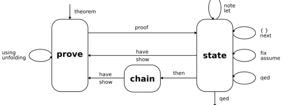
determines the type of transition that may be performed next, it essentially alternates between forward and backward reasoning, with an intermediate stage for chained facts (see figure 2.1).

Figure 2.1: Isar/VM modes

For example, in state mode Isar acts like a mathematical scratch-pad, ac-cepting declarations like fix, assume, and claims like have, show. A goal statement changes the mode to prove, which means that we may now refine

the problem via unfolding or proof. Then we are again in state mode of

a proof body, which may issue show statements to solve pending sub-goals. A concluding qed will return to the original state mode one level upwards. The subsequent Isar/VM trace indicates block structure, linguistic mode, goal state, and inferences:

haveA −→B proof assumeA showB hproofi qed begin begin end end prove state state prove state state (A−→ B) =⇒#(A −→B) (A=⇒ B) =⇒#(A −→B) #(A −→B) A−→ B (init) (resolution impI) (refinement #A =⇒B) (finish)

Here the refinement inference from §2.1.2 mediates composition of Isar sub-proofs nicely. Observe that this principle incorporates some degree of freedom in proof composition. In particular, the proof body allows parameters and assumptions to be re-ordered, or commuted according to Hereditary Harrop Form. Moreover, context elements that are not used in a sub-proof may be omitted altogether. For example:

have V x y.A x =⇒ B y =⇒ C x y proof − fix x and y assume A x and B y showC x y hproofi qed have V x y. A x =⇒ B y =⇒ C x y proof − fix x assume A x fix y assume B y show C x y hproofi qed have V x y.A x =⇒ B y =⇒ C x y proof − fix y assume B y fix x assume A x showC x y sorry qed have V x y. A x =⇒ B y =⇒ C x y proof − fix y assume B y fix x show C x y sorry qed

Such “peephole optimizations” of Isar texts are practically important to im-prove readability, by rearranging contexts elements according to the natural flow of reasoning in the body, while still observing the overall scoping rules. This illustrates the basic idea of structured proof processing in Isar. The main mechanisms are based on natural deduction rule composition within the Pure framework. In particular, there are no direct operations on goal states within the proof body. Moreover, there is no hidden automated reasoning involved, just plain unification.

2.2.4

Calculational reasoning

The existing Isar infrastructure is sufficiently flexible to support calculational reasoning (chains of transitivity steps) as derived concept. The generic proof elements introduced below depend on rules declared as trans in the context. It is left to the object-logic to provide a suitable rule collection for mixed relations of =, <, ≤, ⊂, ⊆ etc. Due to the flexibility of rule composition (§2.1.2), substitution of equals by equals is covered as well, even substitution of inequalities involving monotonicity conditions; see also [54, §6] and [5]. The generic calculational mechanism is based on the observation that rules

such as trans: x = y =⇒ y = z =⇒ x = z proceed from the premises

towards the conclusion in a deterministic fashion. Thus we may reason in forward mode, feeding intermediate results into rules selected from the con-text. The course of reasoning is organized by maintaining a secondary fact called “calculation”, apart from the primary “this” already provided by the Isar primitives. In the definitions below, OF refers to resolution (§2.1.2) with multiple rule arguments, and trans represents to a suitable rule from

the context:

also0 ≡ note calculation = this

alson+1 ≡ note calculation = trans [OF calculation this] finally ≡ also fromcalculation

The start of a calculation is determined implicitly in the text: here also sets calculation to the current result; any subsequent occurrence will up-date calculation by combination with the next result and a transitivity rule. The calculational sequence is concluded via finally, where the final result is exposed for use in a concluding claim.

Here is a canonical proof pattern, using have to establish the intermediate results:

have a =b sorry also have. . . = c sorry also have. . . = d sorry finally have a = d .

The term “. . .” above is a special abbreviation provided by the Isabelle/Isar

syntax layer: it statically refers to the right-hand side argument of the pre-vious statement given in the text. Thus it happens to coincide with relevant sub-expressions in the calculational chain, but the exact correspondence is dependent on the transitivity rules being involved.

Symmetry rules such as x = y =⇒ y = x are like transitivities with only one premise. Isar maintains a separate rule collection declared via the sym attribute, to be used in fact expressions “a [symmetric]”, or single-step proofs “assumex = y then have y = x ..”.

2.3

Example: First-Order Logic

theory First_Order_Logic

imports Base

begin

In order to commence a new object-logic within Isabelle/Pure we introduce abstract syntactic categories i for individuals and o for object-propositions. The latter is embedded into the language of Pure propositions by means of a separate judgment.

typedecl i

judgment

Trueprop :: o ⇒ prop (_ 5)

Note that the object-logic judgment is implicit in the syntax: writingA pro-duces Trueprop A internally. From the Pure perspective this means “A is derivable in the object-logic”.

2.3.1

Equational reasoning

Equality is axiomatized as a binary predicate on individuals, with reflexivity as introduction, and substitution as elimination principle. Note that the lat-ter is particularly convenient in a framework like Isabelle, because syntactic congruences are implicitly produced by unification of B x against expressions containing occurrences of x.

axiomatization

equal :: i ⇒ i ⇒ o (infix = 50) where

refl [intro]: x = x and

subst [elim]: x = y =⇒ B x =⇒ B y

Substitution is very powerful, but also hard to control in full generality. We derive some common symmetry / transitivity schemes of equal as particular consequences.

theorem sym [sym]: assumesx =y shows y = x proof − have x =x .. with hx =yishow y = x .. qed

theorem forw_subst [trans]: assumesy =x and B x

shows B y

proof −

from hy =xihave x = y .. from this andh_{B x}i _{show B y ..} qed

theorem back_subst [trans]: assumesB x and x =y

shows B y

proof −

from hx =yiand hB xi show B y ..

qed

theorem trans [trans]: assumesx =y and y = z shows x = z proof − from hy =ziand hx =yi show x = z .. qed

2.3.2

Basic group theory

As an example for equational reasoning we consider some bits of group theory. The subsequent locale definition postulates group operations and axioms; we also derive some consequences of this specification.

locale group =

fixes prod ::i ⇒ i ⇒ i (infix◦ 70) andinv :: i ⇒ i ((_−1) [1000] 999) andunit :: i (1) assumesassoc: (x ◦ y) ◦ z =x ◦ (y ◦ z) andleft_unit: 1 ◦ x =x andleft_inv:x−1 ◦ x = 1 begin theorem right_inv: x ◦ x−1 = 1 proof −

have x ◦ x−1 = 1 ◦ (x ◦ x−1) by (rule left_unit [symmetric]) also have. . . = (1 ◦ x) ◦ x−1 by (rule assoc [symmetric]) also have1 = (x−1)−1 ◦ x−1 by (rule left_inv [symmetric]) also have. . . ◦ x = (x−1)−1 ◦ (x−1 ◦ x) by (rule assoc) also havex−1 ◦ x = 1by (rule left_inv)

also have((x−1)−1 ◦ . . .) ◦ x−1 = (x−1)−1 ◦ (1◦ x−1) by(rule assoc) also have1 ◦ x−1 =x−1 by (rule left_unit)

also have(x−1)−1 ◦ . . . = 1 by (rule left_inv) finally show x ◦ x−1 = 1 .

qed

theorem right_unit:x ◦ 1 = x

have 1 =x−1 ◦ x by(rule left_inv [symmetric])

also havex ◦ . . . = (x ◦ x−1) ◦ x by(rule assoc [symmetric]) also havex ◦ x−1 _{= 1by (rule right_inv)}

also have. . . ◦ x =x by (rule left_unit) finally show x ◦ 1 = x .

qed

Reasoning from basic axioms is often tedious. Our proofs work by producing various instances of the given rules (potentially the symmetric form) using the pattern “have eq by (rule r)” and composing the chain of results via also/finally. These steps may involve any of the transitivity rules declared in §2.3.1, namelytrans in combining the first two results inright_inv and in the final steps of both proofs, forw_subst in the first combination of right_unit, and back_subst in all other calculational steps.

Occasional substitutions in calculations are adequate, but should not be over-emphasized. The other extreme is to compose a chain by plain transitivity only, with replacements occurring always in topmost position. For example:

have x ◦ 1 =x ◦ (x−1 ◦ x) unfolding left_inv .. also have. . . = (x ◦ x−1) ◦ x unfolding assoc .. also have. . . = 1 ◦ x unfolding right_inv .. also have. . . = x unfolding left_unit .. finally have x ◦ 1 = x .

Here we have re-used the built-in mechanism for unfolding definitions in order to normalize each equational problem. A more realistic object-logic would include proper setup for the Simplifier (§9.3), the main automated tool for equational reasoning in Isabelle. Then “unfoldingleft_inv ..” would become “by (simp only: left_inv)” etc.

end

2.3.3

Propositional logic

We axiomatize basic connectives of propositional logic: implication, disjunc-tion, and conjunction. The associated rules are modeled after Gentzen’s system of Natural Deduction [16].

axiomatization

imp :: o ⇒ o ⇒ o (infixr −→ 25)where

impI [intro]: (A =⇒ B) =⇒ A −→ B and

impD [dest]: (A −→ B) =⇒ A =⇒ B

disj :: o ⇒ o ⇒ o (infixr ∨ 30)where

disjI₁ [intro]: A =⇒ A ∨ B and

disjI₂ [intro]: B =⇒ A ∨ B and

disjE [elim]: A ∨ B =⇒ (A =⇒ C) =⇒ (B =⇒ C) =⇒ C

axiomatization

conj :: o ⇒ o ⇒ o (infixr ∧ 35)where

conjI [intro]: A =⇒ B =⇒ A ∧ B and

conjD₁:A ∧ B =⇒ A and

conjD2:A ∧ B =⇒ B

The conjunctive destructions have the disadvantage that decomposingA∧B involves an immediate decision which component should be projected. The more convenient simultaneous eliminationA ∧B =⇒(A=⇒B =⇒C) =⇒ C can be derived as follows:

theorem conjE [elim]: assumesA ∧ B

obtains A andB

proof

from h_A∧ _Bi _{show Aby (rule conjD1)} from hA∧ Bi show B by(rule conjD₂) qed

Here is an example of swapping conjuncts with a single intermediate elimi-nation step:

assume A ∧ B

then obtain B andA .. then have B ∧ A ..

Note that the analogous elimination rule for disjunction “assumes A ∨ B obtains A B” coincides with the original axiomatization ofdisjE.

We continue propositional logic by introducing absurdity with its character-istic elimination. Plain truth may then be defined as a proposition that is trivially true. axiomatization false ::o (⊥) where falseE [elim]: ⊥=⇒ A definition true :: o (>) where > ≡ ⊥ −→ ⊥

theorem trueI [intro]: >

unfolding true_def ..

Now negation represents an implication towards absurdity:

definition

not :: o ⇒ o (¬_ [40] 40)where

¬ A ≡A −→ ⊥

theorem notI [intro]: assumesA =⇒ ⊥

shows ¬ A

unfolding not_def

proof assume A

then show ⊥by (rule hA =⇒ ⊥i) qed

theorem notE [elim]: assumes¬ A and A

shows B

proof −

from h¬Ai haveA −→ ⊥ unfolding not_def . from h_A−→ ⊥i _andh_Ai_have ⊥ _..

then show B .. qed

2.3.4

Classical logic

Subsequently we state the principle of classical contradiction as a local as-sumption. Thus we refrain from forcing the object-logic into the classical perspective. Within that context, we may derive well-known consequences of the classical principle.

locale classical = assumesclassical: (¬ C =⇒ C) =⇒ C begin theorem double_negation: assumes¬ ¬ C shows C

proof (rule classical) assume ¬ C

qed

theorem tertium_non_datur: C ∨ ¬ C

proof (rule double_negation) show ¬ ¬ (C ∨ ¬C) proof

assume ¬(C ∨ ¬C) have¬ C

proof

assume C then have C ∨ ¬C .. with h¬ (C ∨ ¬C)ishow ⊥ .. qed then have C ∨ ¬ C .. with h¬ _(C ∨ ¬ _C)i_show ⊥_.. qed qed

These examples illustrate both classical reasoning and non-trivial proposi-tional proofs in general. All three rules characterize classical logic indepen-dently, but the original rule is already the most convenient to use, because it leaves the conclusion unchanged. Note that (¬ C =⇒ C) =⇒ C fits again into our format for eliminations, despite the additional twist that the context refers to the main conclusion. So we may write classical as the Isar state-ment “obtains ¬ thesis”. This also explains nicely how classical reasoning really works: whatever the main thesis might be, we may always assume its negation!

end

2.3.5

Quantifiers

Representing quantifiers is easy, thanks to the higher-order nature of the underlying framework. According to the well-known technique introduced by Church [14], quantifiers are operators on predicates, which are syntactically represented as λ-terms of type i ⇒ o. Binder notation turns All (λx. B x) into ∀x. B x etc.

axiomatization

All :: (i ⇒ o) ⇒ o (binder∀ 10) where

allI [intro]: (V

x.B x) =⇒ ∀x. B x and

allD [dest]: (∀x. B x) =⇒ B a

axiomatization

exI [intro]: B a =⇒ (∃x. B x) and

exE [elim]: (∃x.B x) =⇒ (V

x.B x =⇒ C) =⇒ C

The statement of exE corresponds to “assumes ∃x. B x obtains x where

B x” in Isar. In the subsequent example we illustrate quantifier reasoning involving all four rules:

theorem

assumes∃x.∀y. R x y

shows ∀y. ∃x.R x y

proof —∀ introduction

obtainx where∀y. R x y usingh∃_x. ∀_{y.R x y}i _.. — ∃ elimination fix y have R x y using h∀y. R x yi.. — ∀ destruction

then show ∃x.R x y .. —∃ introduction

qed

2.3.6

Canonical reasoning patterns

The main rules of first-order predicate logic from §2.3.3 and §2.3.5 can now be summarized as follows, using the native Isar statement format of §2.2.2.

impI: assumes A =⇒ B shows A −→ B impD: assumes A −→ B and A shows B disjI1: assumes A shows A ∨ B

disjI2: assumes B shows A ∨ B

disjE: assumes A ∨ B obtains A B conjI: assumes A and B shows A ∧ B conjE: assumes A ∧ B obtains A and B falseE: assumes ⊥ shows A

trueI: shows >

notI: assumes A =⇒ ⊥ shows ¬ A notE: assumes ¬ A and A shows B allI: assumes V

x. B x shows ∀x. B x allE: assumes ∀x. B x shows B a exI: assumes B a shows ∃x. B x

exE: assumes ∃x. B x obtains a where B a

This essentially provides a declarative reading of Pure rules as Isar reasoning patterns: the rule statements tells how a canonical proof outline shall look like. Since the above rules have already been declared as intro, elim, dest — each according to its particular shape — we can immediately write Isar proof texts as follows:

have A−→ B

proof assume A

showB hproofi

qed

have A−→ B and A hproofi

then have B .. have A hproofi then have A ∨ B .. have B hproofi then have A ∨ B .. have A ∨ B hproofi then have C proof assume A

then show C hproofi

next

assume B

then show C hproofi

qed have Aand B hproofi

then have A ∧ B ..

have A ∧ B hproofi

then obtain A and B .. have ⊥ hproofi then have A .. have >.. have ¬A proof assume A

then show ⊥ hproofi

qed

have ¬ A andA hproofi

then have B .. have ∀x.B x proof fix x showB x hproofi qed have ∀x. B x hproofi then have B a .. have ∃x.B x proof showB a hproofi qed have ∃x. B x hproofi

then obtain a where B a ..

Of course, these proofs are merely examples. As sketched in §2.2.3, there is a fair amount of flexibility in expressing Pure deductions in Isar. Here the

user is asked to express himself adequately, aiming at proof texts of literary quality.

General Language Elements