Structured Reverse Mode Automatic Differentiation in Nested Monte Carlo Simulations

(1)

Structured Reverse Mode Automatic

Differentiation in Nested Monte Carlo

Simulations

by

An Zhou

A thesis

presented to the University of Waterloo in fulfillment of the

thesis requirement for the degree of Master of Mathematics

in

Applied Mathematics

Waterloo, Ontario, Canada, 2017 © An Zhou 2017

(2)

I hereby declare that I am the sole author of this thesis. This is a true copy of the thesis, including any required final revisions, as accepted by my examiners.

(3)

Abstract

In many practical large scale computational problems, the calculation of partial deriva-tives of the object functionf with respect to input parameters are entailed and the dimen-sion of inputs n is much larger the one of outputs m. The use of reverse mode automatic differentiation (AD) is mostly efficient as it computes the gradient in the same amount of runtime asf regardless of the input dimensionn. However, it demands excessive memory. To enjoy the runtime efficiency of reverse mode without paying unaffordable memory, struc-tured reverse mode has been proposed and succeeded in several applications. Due to the fundamental difficulty in automatic structure detection, structured reverse mode has not been fully automated. This thesis, instead of trying to solve to structure detection problem for a completely generic piece of code, is devoted to the analysis and implementation of deploying structured reverse mode to a generic class of problems with a known structure, nested Monte Carlo simulations. We reveal the general structure pattern of Monte Carlo simulations in financial applications. Space/time tradeoff on deploying structured reverse mode are discussed in details and numerical experiments using Variable Annuity program are conducted to corroborate the analysis. Significant memory and runtime reductions are observed. We argue such contribution is important as nested Monte Carlo simulations accommodates several large scale computations in financial services that are crucial in practice.

(4)

Acknowledgements

I would like to thank all people who made this possible.

Special thanks to my supervisor Thomas F. Coleman for continuous support and guid-ance, and generosity of providing the license of the commercial Automatic Differentiation Matlab package: ADMAT 2.0.

Special thanks for Global Risk Institute for supporting the research involving Variable Annuities where part of this thesis is completed.

(5)

Dedication

(6)

List of Tables

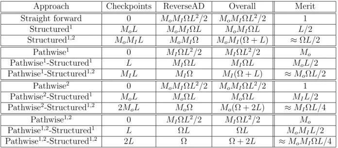
3.1 Comparison of rates of efficiency of different approaches to calculate deriva-tives of a Monte Carlo program . . . 27 5.1 Approaches and their space requirement decomposition for VA problem.

All space are in units of σ0, the space needed to store 1 state vector of the problem. Mo, MI, L 1 is assumed and subleading term is neglected.

LΩ_>1. . . 51 5.2 Comparison of runtime and memory of different approaches on the same VA

program. MaturityT = 25, i.e. length of pathL= 25. Mo = 5,MI = 1000,

N = 2. . . 57 C.1 Algorithm examples with their rate of efficiencies. 1st and 3rd algorithm

are essentially the sampling algorithm of the 2nd and 4th Monte Carlo al-gorithms. . . 75

(11)

List of Figures

2.1 Efficient frontier of the runtime ratio and space tradeoff of the uniform code

c0 when χ0m= 4.5,Ω0k= 7000, S0e= 0.01 . . . 21

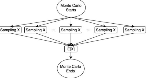
3.1 Parallel structure of generic Monte Carlo algorithm estimating the mean of random variable X . . . 31

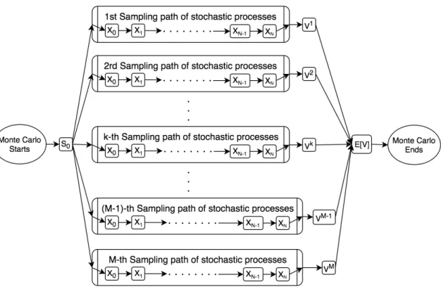
3.2 Sequential path structure of Monte Carlo using an European put option pricing example . . . 32

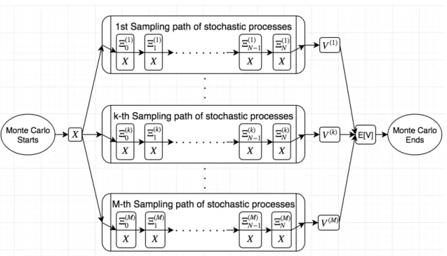
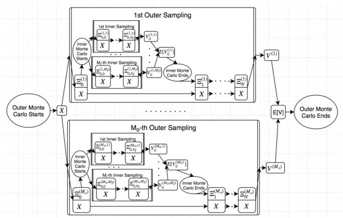
3.3 Abstract sequential path structure of Monte Carlo in financial applications 33 3.4 Abstract nested Monte Carlo simulation in financial applications . . . 35

4.1 High level process of pricing and risk managing VA, credit from Anthony Vaz’s Linkedin page’s PPT Complexities of Variable Annuity Management, page 28 . . . 38

4.2 Wrapping up state vectors and parameters of the VA program . . . 43

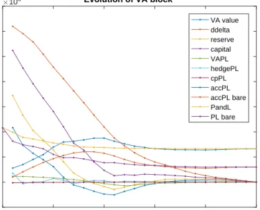
5.1 Demonstration of the evolution of VA block . . . 55

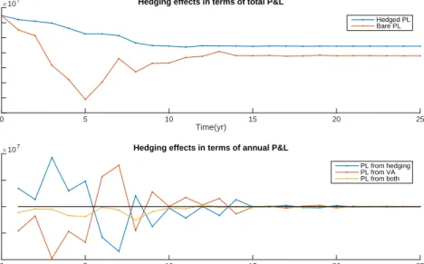
5.2 Demonstration of hedging effect on VA product . . . 56

5.3 Runtime ratio comparison between forward mode and reverse mode on a scalar function using VA program . . . 57

B.1 Demonstration of Naive Reverse Mode: see text for detailed explanation. . 70 B.2 Demonstration of Structured Reverse Mode: see text for detailed explanation. 71

(12)

Chapter 1 Background and Motivation

In various large scale computations, the target function is a scalar or of low dimensional with a much higher dimensional input, and derivatives calculation is entailed. In such scenarios, reverse mode automatic differentiation (AD) becomes the unique choice due to its superior runtime efficiency over alternative approaches such as forward mode AD and finite difference. However, reverse mode’s excessive memory requirement may impede its deployment for large scale computations. Structured reverse mode, an general approach to relax reverse mode’s memory requirement while maintaining reverse mode’s celebrated runtime efficiency, has been proposed but yet to be automated. Case dependent studies have proven structured reverse mode’s effectiveness, yet there has not been any systematic investigations on its deployment to a generic class of computational problems, nested Monte Carlo simulations. In this thesis, we reveal structures of nested Monte Carlo simulations and research how to best utilize such generic structure pattern to achieve efficient reverse mode computation. Numerical experiments using Variable Annuities are conducted and significant memory reduction are found in accordance with theoretical analysis.

1.1 Why Automatic Differentiation?

1.1.1 Importance and cost of Derivatives

In numerous computational applications, in addition to the function value of a continuous functionf, its (partial) derivatives with respect to the inputs are also required.

(13)

In optimization where the target function is to be minimized, we use derivatives (gradi-ent and Hessian) to sketch the local profile of the optimized function, guiding the algorithm towards the next iterative point. The vanishing of first order derivatives signals a local extremum and the positive definiteness of the second order derivatives confirms the genuine-ness of the local minimum. The use of derivatives is ubiquitous in non-linear optimization. In financial applications, the target function is usually the present value of a financial instrument, whether obtained from PDE approach or Monte Carlo simulation. There we need its derivatives with respect to a list of parameters, such as current price, volatility, interest rate, time etc., to hedge away the corresponding risk exposures they represent. Derivative information is often needed for the sake of risk management and reporting pur-poses as well.

As crucial as derivatives are among those applications, the calculation of derivatives takes a longer time to run than the original function itself, whose run time may already be prohibitive. To quantify that the cost of computing the derivatives, the following notations are introduced:

Definition 1.1. ω(c)stands for the runtime of the source codecin a default environment. Definition 1.2. ω(∂ac) stands for the runtime to calculate the derivatives of the

differ-entiable function fc, which the source code c represents, using approach a in a default

environment.

The phrase ‘in a default environment’ is crucial as runtime critically depends on the pro-gramming languages used, the computational power of the machine and also the software packages deployed.

Definition 1.3. The Runtime Ratio of an approach a to calculate the derivatives of the differentiable function fc that a source code c represents is defined as:

Ta(c)≡

ω(∂ac)

ω(c) (1.1)

Such a ratio measure removes most language and machine dependency. Supposefc has

nc _{scalar inputs and} _mc _{scalar outputs, i.e.} _f c : Rn

c

→ Rmc

. By ‘derivatives’, we mean the JacobianJij = _∂x∂zi_j, i∈ {1,· · · , mc}, j ∈ {1,· · · , nc}, z =fc(x). 1

1_{Depending on the problem, sometimes only derivatives with respect to a subset of input variables are}

needed. In such case, we consider the input variables whose derivatives with respect to are not requested

(14)

Finite difference (FD) calculates approximations to the derivatives. However, FD only calculates derivatives with respect to one input at each run, i.e.:

TF D(c)≈

(

nc_, _Forward_/_{Backward difference}

2nc_, _{Central difference} (1.2)

When the dimension of the input is too large–larger than 103 _{for example–using FD}

to obtain derivatives becomes impractical. One famous example is the stagnation of the artificial neural network field in the 70s after Marvin Minsky and Seymour Papert pub-lished Perceptrons: An Introduction to Computational Geometry where they ‘showed’ the

training of deep neural networks is practically impossible due to large number of inputs. For instance, modern deep neural networks can have parameters up to 107. For complex

financial applications such as LIBOR model,104₋₁₀6 _{inputs scalars of which derivatives}

are requested are common. When the original function already has a prohibitive runtime, obtaining the derivatives with runtime ratio more than104 is unacceptable. Reverse mode

AD rides to the rescue.

1.1.2 Reverse mode Automatic Differentiation

AD calculates the derivatives exactly and automatically[1]. Furthermore, reverse mode AD[2] computes the gradient within constant runtime ratio, regardless of number of inputs.

In Griewank’s On Automatic Differentiation[3], it reads:

“...Thus we can conclude that under quite realistic assumptions the evaluation of a gradient requires never more than five times the effort of evaluating the underlying function itself...”

It is such guaranteedO(1)runtime ratio scaling that opens the doors for efficient

deriva-tive calculations in large scale optimizations[4] and financial instrument pricing[5][6][7]. More precisely:

TRev(c) = χ(c) (1.3)

where χ(c) is a factor that depends on the details of c however is upper-bounded as Griewank stated: χ ₆ 5. The crucial difference with TF D(c) is that it scales with mc

(15)

but notnc.

We should note that gradient means specifically the derivatives of a scalar function. Indeed, for most applications, target function whose derivatives are of interest is scalar. In optimization,f is scalar simply because only scalar has natural order therefore can be optimized. In finance, the present value of an instrument is a scalar as well.

1.2 Why Structured Reverse Mode?

1.2.1 Bottleneck of Reverse Mode in large scale computation

Reverse mode calculates derivatives with respect to all inputs at once. However, this is at the cost of memory: a typical space/runtime tradeoff. Reverse mode literally evaluates the derivatives of the original function in a backwards fashion which requires saving all the intermediate variables, potentially demanding a much larger memory than the one needed for the original function evaluation.

Definition 1.4. σ(c) is the amount of memory needed for executing c, in units of bytes, in a default environment.

Definition 1.5. σ(∂ac) is the amount of memory needed for computing the derivatives

of the function fc, which the source code c represents, using approach a in a default

environment.

Similar to runtime, the size of memory depends on the programming language used2_.

Definition 1.6. The Space ratio of an approach a to calculate the derivatives for the differentiable function fc that a source code c represents is defined as:

Sa(c)≡

σ(∂ac)

σ(c) (1.4)

Such a ratio measure largely removes the programming language dependency.

2_{As basic data types are implemented differently and different memory management schemes (static or}

(16)

The bottleneck for reverse mode is that such space ratioSRev(c)as defined above can be

excessive, typically scaling linearly with the depth of the original function. Such memory requirement is the bottleneck to apply reverse mode for modern large scale computations, motivating the birth of structured reverse mode.

1.2.2 Structured Reverse Mode

To tackle the extensive space requirements that reverse mode suffers, systematic approaches have been developed [8][9][10]. The space requirements of reverse mode comes from the fact that all intermediate variables during the entire computation need to be saved such that we can propagate the derivatives backwards. To release spaces, only a subset of variables are stored, i.e. checkpoints, which are chosen such that original computational graph can be recovered as we propagate the derivatives. Such method is called ‘checkpointing’ or ‘structured reverse mode’, since observation of the structural pattern off’s source code is critical for the approach to be effective.

Checkpointing can significantly relax the space requirements of reverse mode at a marginal cost of runtime and can be deployed recursively. For 1 level of checkpointing, denoted as approach “StrRev”, only 1 additional run off is done. We have:

ω(∂StrRevc) = ω(∂Revc) +ω(c) (1.5)

hence:

TStrRev(c) =TRev(c) + 1 = 1 +mc·χ(c) (1.6)

The additional function run reduces the memory to: σ(∂StrRevc)∼ p σ(∂Revc)σ(c) (1.7) hence: SStrRev(c)∼ p SRev(c) (1.8)

The bigger picture is: reverse mode obtains great time efficiency at the cost of space. Yet it is an extreme case of time/space tradeoff. Structured reverse mode offers a generalized spectrum of the same tradeoff with naive reverse mode as a special case. What is remarkable is that by increasingT by 1,Sis reduced exponentially compared to straight forward reverse mode.

(17)

1.3 How to structure Reverse Mode

Structured Reverse Mode seems to be the holy grail for large scale computation: it resolves the memory overflow issue of reverse mode and maintain its powerful runtime efficiency. However, the performance of structured reverse mode depends on what structure is de-ployed, in other words, how checkpoints are selected. There’s no exploitable structure for a generic piece of code and for certain codes, though unlikely a practical one, that the structured reverse mode does not improve over reverse mode itself at all.

People have made progress on algorithms that automatically find optimal positions of checkpoints to truly automate structured reverse mode [11][12][13]. Unfortunately, the automation has yet to achieve full generality. So far, even if a natural checkpointing ofc exists, there’s no guarantee that the algorithm would find it.

Motivation of this thesis: Instead of focusing on algorithms that can automatically detects code structure, we research on how to best deploy structured reverse mode with a given structure. Such structure is general, and in fact, for any nested simulations in finan-cial applications. Variable Annuities, as a practical example, has the according structure and will be used for numerical experiments.

1.4 Guide to the reader

The thesis is organized in the following way: Chapter I motivates the thesis; Chapter II presents the idea of structured reverse mode automatic differentiation and discusses how different uses of structure affect the tradeoff between space and runtime; Chapter III discusses the use of Monte Carlo simulations in financial applications, its rate of efficiency and its structure; Chapter IV provides the technical background for Variable Annuities program and reveal its structure; Chapter V, the core part of the thesis, is dedicated to the deployment of structured reverse mode in nested simulation with theoretical analysis and numerical experiments; Appendix contains the technical details that are entailed to make the thesis self-contained.

(18)

Chapter 2 Structured Reverse Mode

In this chapter, we explain the basic framework and computational aspects of AD, and introduce the idea and mathematics of structured reverse mode using a simple uniform sequential program.

2.1 Understanding Reverse Mode

AD comes from the observation that any code at runtime1 _{is an ordered collection of basic}

analytic operations. The derivatives of the basic operations2 are easy to compute. If we

compute the derivatives for all the basic operations involved and process them as dictated by the chain rule, we shall arrive at the exact derivatives. Let’s use such a framework to

decompose a given source code c.

2.1.1 Decomposition of source code

For an arbitrary given source code c of a differentiable function f : Rn _{→ R}m, denote

its input as x ∈ Rn _{and output as} _z _{∈ R}m_{. The code at runtime can be decomposed}

1_{Notice the clause “at runtime” is crucial. Codes typically have loops and conditional expressions. We}

don’t know exactly what part of the code will be executed, how many times that a particular snippet of code would be run, and what are the specific order of execution before completing the code’s execution. What we are referring to is the resulting computations of the source code.

(19)

chronologically as:                y1 =b1(Arg1) =b1(x) y2 =b2(Arg2) ... yk−1 =bk−1(Argk−1) z =bk(Arg_k) (2.1)

kis the total number of basic operations thatf is composed of, which depends on the input x in general. Arg_i stands for the set of non-constant3 arguments given to the elementary

function bi (b stands for basic). Every bi is a basic operation, hence it takes either 1 or 2

arguments.

With the above understanding, we have: ∀i∈ {1,· · · , k}

(

|Arg_i| ∈ {1,2}

Arg_i ∈ {x, y1,· · · , yi−1}

(2.2)

3_{We don’t consider constants as intermediate variables} _{y. By constant, we mean anything that does}

(20)

2.1.2 Calculation of Jacobian

When AD is invoked, derivatives of all the basic operations{b}are calculated and assigned properly in the following extended Jacobian matrix JE of {bi}ki=1:

JE ≡               ∂b1 ∂x −I O · · · O ∂b2 ∂x ∂b2 ∂y1 −I ... · · · ... ∂b3 ∂x ∂b3 ∂y1 ∂b3 ∂y2 −I ... · · · ... ... ... ... ... ... ... ... ∂bk−2 ∂x ∂bk−2 ∂y1 ∂bk−2 ∂y2 · · · ∂bk−2 ∂yk−3 −I O ∂bk−1 ∂x ∂bk−1 ∂y1 ∂bk−1 ∂y2 · · · · ∂bk−1 ∂yk−2 −I ∂bk ∂x ∂bk ∂y1 ∂bk ∂y2 · · · · ∂bk ∂yk−1               ≡ A B C D (2.3) A= (∂b1 ∂x) T_,_{· · ·} _,₍∂bk−1 ∂x ) TT B =            −I O · · · O ∂b2 ∂y1 −I ... · · · ... ∂b3 ∂y1 ∂b3 ∂y2 −I ... · · · ... ... ... ... ... ... ... ∂bk−2 ∂y1 ∂bk−2 ∂y2 · · · ∂bk−2 ∂yk−3 −I O ∂bk−1 ∂y1 ∂bk−1 ∂y2 · · · · ∂bk−1 ∂yk−2 −I            C = ∂bk ∂x D=∂bk ∂y1 · · · ∂bk ∂yk−1 (2.4) Notice thatx,y,b(·)might be vectors hence each block inJE, A, B, C, Dmight be matrices.

I and O are identity matrix and matrix of all zero of appropriate size. Denoting ni as yi’s

dimension, i.e. bi’s output dimension, _∂y∂bi_j would be a ni ×nj matrix. B is lower block

triangular and has identity matrix along the diagonals, hence non-singular. B is also sparse for eachb takes at most 2 arguments, i.e. each row has no more than 3 non-zero elements. By definition: ( Adx+Bd{y} = 0 Cdx+Dd{y} =dz ⇒dz = (C−DB −1_A₎_dx _≡_{J dx} _(2.5) {y}= yT 1,· · · , ykT−1 T

(21)

where we have denoted y in column vectors forms. Such computation is related to the Schur complement of JE’s submatrix. Hence the derivatives are computed as:

J =C−DB−1A (2.6)

2.1.3 Intuitive example

Readers that are familiar with reverse mode may skip this section. Consider a simple

sequential codec∗ that calculates f∗ with the following structure:

Arg∗_i+1 =

(

{x} i= 0

{y∗_i} otherwise (2.7)

We will use∗ _{superscript to indicate reference to the special sequential case of}_f∗_{. Due to}

the structure in Arg∗_i,A∗, b∗, C∗, D∗ can be simplified: A∗ =(∂b∗1 ∂x) T_{, O,}_{· · ·} _{, O}T b∗ =             −I O · · · O ∂b∗₂ ∂y1 −I ... · · · ... O ∂b∗3 ∂y2 −I ... · · · ... ... ... ... ... ... ... ... ... ... ∂b∗_k₋₂ ∂yk−3 −I O O · · · O ∂b ∗ k−1 ∂yk−2 −I             C∗ =O D∗ =O, · · ·, O, ∂b∗k ∂yk−1 (2.8) Hence the Jacobian can be explicitly calculated as:

J∗ =C∗−D∗(B∗)−1A∗ = ∂b ∗ k ∂y∗ k−1 · ∂b ∗ k−1 ∂y∗ k−2 · · ·∂b ∗ 2 ∂y∗ 1 · ∂b ∗ 1 ∂x (2.9)

as expected. Now how would AD compute the above product for each of the two modes? Reverse mode has a forward sweep and a backward sweep where forward mode only have the forward phase. For the forward phase in both modes, ∂b∗_i+1

(22)

Forward mode AD keeps updating ∂y_i∗

∂x and stores the results. In this example, once ∂b∗_i+1

∂y∗

i is obtained, forward mode left multiplies it to ∂b∗_i

∂y∗

i−1 · · ·

∂b∗₁

∂x then stores the result as ∂y∗

i+1

∂x .

In contrast, reverse mode simply stores all the ∂b∗

i+1

∂y∗

i and does not do any computation in the forward phase. In the backwards phase, reverse mode computes backwards, i.e. ∂b∗_i

∂y_i∗−1 is multiplied to the right of ∂b∗_k

∂y_k∗−1

· · ·∂b∗i+1

∂y∗_i until the whole product is done. Let’s inspect

the runtime complexities of both modes.

• Forward mode: The above matrix products are time ordered from right to left, which is order the forward mode operates. It first left multiplies ∂b∗

2

∂y∗₁ to ∂b∗

1

∂x.

Recall-ing the complexity of multiplyRecall-ing a a×b matrix to a b×c matrix is O(abc), ∂b∗2

∂y₁∗ is

of sizen2×n1and ∂b∗₁

∂x is of sizen1×n, such multiplication givesO(nn1n2)complexity.

The resulting matrix ∂b∗2

∂y∗₁ ∂b∗1

∂x is now of size n2×n. Then ∂b∗3

∂y∗₂ is left multiplied to get ∂b∗3 ∂y∗ 2 ∂b∗2 ∂y∗ 1 ∂b∗1

∂x of size n3×n with O(nn2n3) operations. So on and so forth.

Hence overall runtime complexity of forward mode is: ω(∂Forc∗)∼n·[

k−2

X

i=1

nini+1+nk−1m] (2.10)

• Reverse mode: As explained, the first computation would be ∂b∗k

∂y∗ k−1 · ∂b ∗ k−1 ∂y∗ k−2 which takes O(mnk−1nk−2)resulting in a matrix of sizem×nk−2. And thenO(mnk−2nk−3)

to a m×nk−3 matrix. So on and so forth.

Hence overall complexity for reverse mode is: ω(∂Revc∗)∼m·[

k−2

X

i=1

nini+1+n1n] (2.11)

We see reverse mode and forward mode scales differently. k1, hencePk−2

i=1 nini+1 n1n

and Pk−2

(23)

complexity expressions are asymptotically the same. In fact, ω(c∗)∼n1n+ k−2 X i=1 nini+1+nk−1m (2.12)

represents the complexity of the function itself (since a step from y∗_i to y_i+1∗ generally has complexity nini+1). Now we can tell why reverse mode is more efficient when the input

dimension is large and the output dimension is small. When computing derivatives forf∗, forward mode’s computations’ matrices always have nc _{columns where as reverse mode’s}

computations involves matrices of mc rows. Other scalings are asymptotically the same.

Forward mode computes the Jacobian matrix one column (each input) at a time while reverse mode computes one row (each output) at a time.

(

TFor(c) ∼nc

TRev(c) ∼mc

(2.13)

∗ _{superscript is dropped since the above is true in general. Note when a gradient is needed,}

i.e. mc_{= 1}, reverse mode computes it at once.

2.2 Structuring Reverse Mode

Having observed the runtime behavior, we inspect the space ratio of both modes of AD. In the above example, forward mode takes storage:

σ(∂Forc∗)∼n k max i=1 {ni}+ k max i=1 {σ(b ∗ i)} (2.14)

since it is keeping ∂yi

∂x. The first term is negligible and the second part is just:

σ(c∗)∼maxk i=1 {σ(b

∗

i)} (2.15)

Hence the space ratio S of forward mode on c∗ is O(1).

SFor(c∗) =

σ(∂Revc∗)

σ(c∗₎ ∼

nmaxk

i=1{ni}+ maxki=1{σ(b ∗ i)} maxk i=1{σ(b ∗ i)} ∼1 (2.16)

(24)

Definition 2.1. The Tape Size σ¯(c) of a source codec is defined as:

¯

σ(c) = Storage needed for all intermediate variables during execution of c

(except those created within basic operations) and the Computational Graph of c (2.17) Definition 2.2. σ(y)is the storage needed to store the variableyin a default environment.

therefore:

σ(∂Revc) = ¯σ(c) (2.18)

For sequential programf∗, we have:

¯ σ(c∗) = k X i=1 ¯ σ(b∗_i)∼ k X i=1 σ(b∗_i) (2.19)

where we have used the fact that B∗ is basic operations hence no intermediate variables are stored and the storage for the type of basic operation have been neglected. Therefore:

SRev(c∗) = σ(∂Revc∗) σ(c∗₎ = ¯ σ(c∗) σ(c∗₎ ∼ Pk∗ i=1σ(b ∗ i) maxk∗ i=1{σ(b∗i)} ∼k∗ (2.20)

reverse mode’s space ratio scales linearly with the depth of the function k∗ whereas the one of forward mode is O(1). The O(k) space ratio may impede the use of reverse mode

for large scale computations despite its significant runtime advantages. Let’s see how structured reverse mode reduces the undesirable space complexity of reverse mode while maintaining its runtime efficiency.

2.2.1 Basic Idea of Checkpointing

Reverse mode’s space complexity comes from storing all intermediate variables that a pro-gram have ever created. If such storage is not kept, the derivatives cannot be successfully propagated in the backward phase. However, viewing the whole program as a concatena-tion of multiple subprograms, divide and conquer can be deployed.

The original idea of multilevel differentiation is found in [8] and further developed in [10]. Only the checkpoint variables, instead of all, are stored in the forward sweep. During

(25)

backward sweep, reverse mode is applied to the tape segments between checkpoints one at a time. Obtaining the checkpoints needs one additional evaluation of the original function. Therefore time ratio T only increase by 1 however the space ratio S is reduced exponen-tially, as it turns out for a typical code.

Checkpoints{Pi} np

i=1 are essentially an ordered collection of subsets of all intermediate

variables {yi}ki=1. However, not any ordered collection of subsets of {yi}ki=1 qualifies as a

set of checkpoints. As the full formulation involves cumbersome notations and is not of importance for the following discussion, we leave it to Appendix B.1 and only states its definition and the qualifying property.

Definition 2.3. Given a codec, its inputx, outputzand all intermediate variables{yi}ki=1

in c’s resulting computation, a selection of checkpoints{Pi} np+1

i=0 is an ordered collection of

subsets of {yi}ki=1 s.t.:          P0 ={x} Pi ⊆ {yi}ki=1 ∀i∈ {1,· · · , np} Pnp+1 ={z} Pi < Pi+1 ∀i∈ {1,· · · , np−1} (2.21)

where P1 < P2 means∀y∈P1 and∀y0 ∈P2, yappears strictly chronologically earlier than

y0 in the execution of c.

Definition 2.4. A selection of checkpoints {Pi} np+1

i=0 of code c is admissible if there exist

code{Wi} np+1

i=1 s.t. the following ordered execution has exactly the same set of intermediate

variables as c:                y1 =b1(Arg1) =b1(x) y2 =b2(Arg2) ... yk−1 =bk−1(Argk−1) z =bk(Argk) ⇔                P1 =W1(P0) = W1(x) P2 =W2(x, P1) ... Pnp =Wnp(x, P1,· · · , Pnp−1) z =Pnp+1 =Wnp+1(x, P1,· · · , Pnp) (2.22)

The set of all y and empty set _∅ are two trivial admissible selections of checkpoints. All discussions afterwards will be based on an admissible selection of checkpoints. Now we

(26)

Algorithm 1Structured Reverse Mode

function _{strReverseMode}(x, Code c, Admissible selection of checkpoints {Pi} np

i=1)

Evaluate the code conce and store {Pi} np

i=1.

Apply reverse mode on code segment Wnp+1. Then on Wnp etc. Until we fully propagate the derivatives to x.

end function

calculate what runtime and space ratio can be achieved for reverse mode. The algorithm of structured reverse mode given{Pi}

np

i=1 is simply 4_:

For illustration of structured reverse mode, see Appendix B.3. By saving only{Pi} np

i=1,

space complexity is reduced. Storage comes from two parts5_{: (a) storage of checkpoints}

(b) storage of intermediate variables during reverse mode on each segment Wi. Hence:

σ(∂StrRevc) = np X i=0 σ(Pi) + np+1 max i=1 σ(∂RevWi) = np X i=0 σ(Pi) + np+1 max i=1 ¯σ(Wi) (2.23)

We see there is tradeoff in the density of checkpoints. The first term would increase if we increase the density and the second term would increase if we decrease the density.

For runtime, we have an additional run ofcregardless of the selection of the checkpoints. ω(∂StrRevc) = ω(c) +ω(∂Revc)

as we mentioned in the first chapter.

2.2.2 A program of uniform checkpoint structure

In previous subsection, we defined what is an admissible selection of checkpoints and cal-culated the runtime and space of the structured approach. However, all are rather abstract and general, therefore hard to quantify. The objective of this subsection is to understand what checkpoints arrangement yields desirable space and runtime ratio overall. Let’s study a uniform program in which quantities of interest can be easily computed therefore several useful insights can be drawn.

4_{The detailed numerical procedure of “derivatives propagation” can be found in Appendix} _A_.

5_{The storage required by the original function evaluation} _σ₍_c₎ _{is neglected since it is negligible for}

(27)

Suppose the codec0 has been divided by an admissible selection of checkpoints{Pi}ki=1−1

into subprograms{Wi}ki=1. c0 is also‘uniform’ such that runtime and space computation is

simplified: ∀i∈ {1,· · · , k}          ω(Wi) =ω0 χ(Wi) =χ0 σ(Wi) = ˆσ0 ¯ σ(Wi) = ¯σ0 (2.24) ∀i∈ {1,· · · , k−1} σ(Pi) =σ0 (2.25)

Since σ0 is the space to store the input ofW: P,σˆ0 the space needed during computation

of W, andσ¯0 is the full tape of W. It follows that:

σ0 6σˆ0 6σ¯0 (2.26)

It also follows that:

                   ω(c0) =kω0 ω(∂Revc0) =χ0m·kω0 σ(c0) = ˆσ0 σ(∂Revc0) =kσ¯0 TRev(c0) =χ0m SRev(c0) =kσ¯0/σˆ0 (2.27)

As inspired by (2.23), there’s a tradeoff in the density of checkpoints. Empty set, as an admissible checkpoint selection that leads to naive reverse mode, represents the extreme that minimizes the first term (storage of checkpoints) and reaching the maximum of the second term (storage for reverse mode on subprograms). The set of ally is the other ex-treme, minimizes the second term (storage for reverse mode on subprograms) and reaching the maximum of the first term (storage of checkpoints). To find a balanced tradeoff with-out worrying abwith-out admissibility, the selection of checkpoints {Pi}ki=1−1 is further assumed

to be Markovian as well6.

Definition 2.5. An admissible selection of checkpoints is Markovian if each of its

repli-cating code segmentsWi+1 only takes xand the previous checkpoint Pi as its input.

(28)

Theorem 2.6. A subset of a Markovian admissible collection of checkpoints is also an Markovian admissible selection of checkpoints.

For proof of Theorem 2.6, see Appendix B.2. In light of Theorem 2.6, any subset {Qi}

np

i=1 of {Pi}ki=1−1 would be admissible. As admissibility is always satisfied, we only need

to find an optimal subset{Qi} np

i=1 to minimize our space cost. Suppose{Qi} np

i=1 divides the

code c0 into {Vi} np+1

i=1 , denoting its indexing of {Pi}ki=1−1 asqi:

∀i∈ {0,· · ·, np+ 1} Qi =Pqi (2.28) The following relation should hold:

0 = q0 < q1 <· · ·< qnp < qnp+1 =k (2.29) Hence (2.23) can be rewritten as:

σ(∂StrRevc0) = np X i=0 σ(Qi) + np+1 max i=1 σ¯(Vi) = (np+ 1)σ0+ ¯σ0· np max i=0 (qi+1−qi) (2.30)

Given a fix number of checkpoints, it is obvious that evenly separated checkpoints are favorable since the first term does not depend on the distribution of Qi, and the second

term can be minimized with equally spaced checkpoints. We assume k 1 and np k

hence the difference betweenfloor(_nk

p+1)and

k

np+1 can be neglected as such difference would be at most a sub-leading term asymptotically.

σ(∂StrRevc0)≈(np+ 1)σ0 + k np + 1 ¯ σ0 >2 p kσ0σ¯0 (2.31)

Hence we see that the optimal number of checkpoints are:

ˆ np = r ¯ σ0 σ0 k−1∼ r ¯ σ0 σ0 k (2.32) ˆ

np indeed scales less than k hence our assumption np k holds. For later convenience,

we denote7_:

S0 =σ0/σˆ0 (2.33)

7_S

0is just a quantity that appears frequently in later formula, not a space ratio of the code piece W:

(29)

Hence using structure halves the order of magnitude of space ratio compared to a straightforward reverse mode and only adds 1 to the runtime ratio:

( TStrRev(c0) = 1 +TRev(c0) = 1 +χ0m SStrRev(c0) ≈2√kσ0σ¯0/σˆ0 = 2 p SRev(c0)S0 (2.34) providing a space efficient alternative to the bare reverse mode.

Notice the dimensionless combination σ¯0

σ0 is a key factor in expressions of nˆp and space ratio S. As σ¯0 is the amount of computation done at each checkpoint, σ0 is the size of

input, it conceptually represents a ratio of “computation per input”:

Definition 2.7. The computation per input (CPI) ratio Ω(c)of a code cis defined as:

Ω(c) = σ¯(c)

σ(xc) (2.35)

wherexc is the input of c.

ForWi, σ_σ¯0₀ is exactly the CPI ratio: Ω(Wi)≡Ω0 = ¯ σ0 σ0 ∀i∈ {1,· · · , k} (2.36)

2.2.3 Recursive structure

We see in (2.34) that for the uniform code c0 of length k, we can apply structured reverse

mode to obtain significant improvement of space ratio by marginally increment in runtime ratio. Just as divide and conquer normally works, such structure can be applied recursively. We relaxnp from beingnˆp, and then apply structured reverse mode withn0p checkpoints

again on each piece of tape Vi. Denoting such 2-level structure to be approach Str2Rev,

we obtain: σ(∂_Str2_Revc₀)≈(n_p+n0_p+ 2)σ₀ + k (np+ 1)(n0p+ 1) ¯ σ0 >(np + 1)σ0+ 2 √ kσ0σ¯0 p np+ 1 >3k13σ 2 3 0σ¯ 1 3 0 (2.37)

(30)

the equal sign is reached when: ( ˆ np = (¯σ_σ0₀k) 1 3 −1∼(¯σ0 σ0k) 1 3 = (Ω₀k) 1 3 ˆ n0_p =q¯σ0 σ0 k ˆ np+1 −1 = ˆnp ∼(Ω0k) 1 3 (2.38)

Interestingly, nˆ0_p = ˆnp exactly. The above optimal number of checkpoints achieves the

following runtime and space ratio: ( TStr2_Rev(c₀) = 1 +T_StrRev(c₀) = 2 +χ₀m S_Str2_Rev(c₀) ≈3k 1 3(σ₀/σˆ₀) 2 3(¯σ₀/σˆ₀) 1 3 = 3S 1 3 Rev(c0)S 2 3 0 (2.39) We can see a pattern already. As a natural generalization, using structure of level l, we would have:        T_Strl_Rev(c₀) =l+χ₀m S_Strl_Rev(c₀) = (l+ 1)k 1 l+1(σ 0/σˆ0) l l+1(¯σ 0/σˆ0) 1 l+1 = (l+ 1)S 1 l+1 Rev(c0)S l l+1 0 S_Strl_Rev(c₀)/S₀ = (l+ 1)(S_Rev(c₀)/S₀) 1 l+1 (2.40) achieved when: n(1)_p =· · · =n(l)_p ≡(σ¯0 σ0 k)l+11 −1∼(σ¯0 σ0 k)l+11 = (Ω 0k) 1 l+1 (2.41)

The consistency condition changes from np k toQl_i=1n (l)

p k, which is satisfied for all

l ∈Z+ since the left hand side scales as_kl/(l+1), which is less than _k.

It might seem meaningless to calculate everything accurately since we are dealing with an artificial example. Also l and the distribution of checkpoint positions represented by np are fundamentally discrete no matter how we pretend they can achieve the non-integer

optimal value.

Yet there are two general conclusions that we can draw: (1) the optimal arrangement of checkpoints is the one that evenly divides the computation (2) to achieve the best space ratio, the optimal level l is not infinity. When too many level of structures are used, more space are actually needed. To find out the best level depth l, we find the argmin with respect to l by taking derivatives of the In of S_Strl_Rev(c₀)/S₀:

0≡ ∂ ∂lIn[ S_Strl_Rev(c₀) S0 ] = ∂ ∂l(In(l+ 1) + 1 l+ 1In[ SRev(c0) S0 ]) = 1 l+ 1 − 1 (l+ 1)2In[ SRev(c0) S0 ]

(31)

which we can solve for the optimalˆ_l_: ˆ

l = In[SRev(c0)

S0

]−1 = In[Ω0k]−1 (2.42)

where we can realize the following runtime and space ratio: ( ˆ TStrRev(c0) = In[Ω0k] +χ0m−1∼lnk ˆ SStrRev(c0) =S0eIn[Ω0k]∼lnk (2.43) with: ˆ np =e−1 (2.44)

Somehoweshows up in a funny way. Of course it is not possible to have non-integer valued number of checkpoints, hencenp = 2 is likely the best choice meaning a tertiary recursive

structure achieves the lowest space ratio.

We conclude that for such code with a uniform Markovian checkpoint structure, recur-sively structured reverse mode gives a logarithmic scaling in terms of function depth k in both runtime and space ratio, in accord with [10].

2.2.4 Efficient frontier of the runtime/space tradeoff

In analogy to portfolio optimization we consider the tradeoff between expected return and variance, an efficient frontier of space/runtime ratio for our uniform program c0 can be

drawn.

The efficient frontier of space/runtime ratio for c0 is given by the following formula:

(

S =S0(T −T0+ 1)(Ω0k)1/(T−T0+1)

T0 =TRev(c0) =χ0m

(2.45) where have useS and T to denote space and runtime ratio respectively.

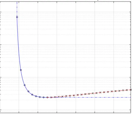
In Figure 2.1, log scale is used for the space ratio. Points on the curve are the pairs of runtime/space ratio achieved with different levels of structures. As noted, runtime ra-tio increases linearly with the level of structure however the space rara-tio does not always

(32)

Runtime ratio (T) 0 5 10 15 20 25 30 Space ratio (S) 10-1 100 101 102

Runtime Space tradeoff of Reverse mode on c

0

Figure 2.1: Efficient frontier of the runtime ratio and space tradeoff of the uniform code c0 when χ0m= 4.5,Ω0k = 7000, S0e= 0.01

decrease. After passing the optimal level depth ˆ_l _{which is about} ₈ _{here (corresponds to}

Runtime ratio T = 8 +χ0m = 12.5), space ratio also goes up when we increase level of

structure (represented by crosses on the red dashed line). Hence the right part of the curve is inefficient in both space and time hence is not on the efficient frontier.

This efficient frontier is different from portfolio analysis setting since we are trying to minimize both space and runtime ratio compared to variance minimization coupled with expected return maximization. Our efficient frontier is of finite size as represented by the unfilled circles on the blue solid curve which are essentially from bare reverse mode to structured reverse mode of level ˆ_l_{. We see the bare reverse has an extremely high space}

(33)

We observe that space ratio can be drastically reduced even when we only have very few layers of structure. The amount of space released per runtime decreases ‘exponentially’ as we increase the level of structure and would turn negative after O(logk) level of layers.

2.2.5 Concluding remarks

We have made a few important observations above. However, they are based on our simple example of a program with uniform Markovian admissible checkpoints, one may wonder which ones of them generalize? As we will see in Chapter 3, for Monte Carlo simulations in financial applications, the program always displays a Markovian admissible checkpoint structure. Hence:

(1) Within each level of structure, the checkpoints should separate the amount of com-putations as evenly as possible.

(2) It is not always beneficial to increase the level of structure. Too many layers of structure are inefficient in both runtime and space and should be avoided.

(3) The first few levels of structure performs best in terms of trading runtime for space reduction. Being easier to implement, just one or two levels could be sufficiently efficient in practice.

We see the choice of structure architecture is not trivial. However, previous discussions are dealing with our simple uniform program example. In practice, even revealing the structure of a given code is non trivial. And it is a lot harder to determine the optimal checkpoints positions when the code segmentsW contain varied amount of computations. In the following Chapter 3 and Chapter 4, we are going to introduce Monte Carlo simula-tions and Variable Annuities. With the ‘structure’ mindset developed in this chapter, we are ready to put their computations into perspectives. In Chapter 5, a general framework of structure design for nested simulations will be formulated.

(34)

Chapter 3 Monte Carlo simulation in Finance

This chapter discusses the convergence of Monte Carlo algorithm, and how different ap-proaches of derivatives calculations lead to distinct rate of efficiency. As reverse mode AD calculates exact derivatives efficiently, forward mode AD calculate exact derivative ineffi-ciently, FD calculates approximations ineffiineffi-ciently, their rates of efficiency show hierarchy. Finally, general structure of Monte Carlo simulations in financial applications are revealed.

3.1 Convergence of Monte Carlo

Monte Carlo methods in general are computational algorithms that obtain certain prop-erties of random variables, mostly the mean, by repeated random sampling on them. The convergence of Monte Carlo algorithm on mean estimation is guaranteed by central the-orem. If we define the following rate of efficiency, a simple Monte Carlo algorithm would haveβmc= 0.5. See Appendix C.1.

Definition 3.1. The rate of efficiency βa ∈(0,∞]of an algorithm a to compute a scalar

quantity y is defined via the following asymptotics1:

|ya−y| ∼O(Ma−βa) (3.1)

where ya is the approximation of y that approach a computes, and Ma is the complexity

of a’s runtime.

1_{For simplicity, float point accuracy is considered} _∞ _{precision. For algorithm with} _O₍₁₎ _complexity

(35)

It can be showed that rate of efficiency of a Monte Carlo deploying approacha to draw samples is: βmc(a) =βmc(a)s = βa 2βa+ 1 ∈(0,1 2] (3.2)

The rate of efficiency of Monte Carlo is naturally the harmonic mean of a’s rate of effi-ciencyβa and the suppose-to-be rate of efficiency of Monte Carloβmc = 0.5. For proof, see

AppendixC.2.

Whereas such rate of efficiency is at most 0.5, Monte Carlo’s rate of efficiency scaling

is excellent for its independence of the problem’s dimensionality2. In finance, Monte Carlo

and PDE are THE3 _{two approaches for pricing financial instruments without analytic}

expressions. PDE scales as:

     |xpde−x| ∼∆xγa Mpde ∼∆x−d βpde =γa/d (3.3) where d is the dimensionality of the problem, γa is the convergence rate of the PDE

approach, which depends on the time stepping method used and the regularity of the priced instrument. Best situation we haveγa = 2resulting in βpde= 2/dwhich still suffers

from the curse of dimensionality despite being superior for d = 1. The best for Monte

Carlo is1/2henced= 4 is usually considered as a critical dimension beyond which Monte

Carlo’s efficiency would be higher than PDE in general.

3.2 Convergence of Monte Carlo derivatives

Monte Carlo estimates the mean of a random variable. However in many applications, derivatives of the mean are requested as well. Finite difference provides the most natural approximation and is easy to implement. Automatic differentiation computes the exact derivatives of each sample automatically. Let’s compute their rates of efficiency.

2_{Dimensionality might affect implicitly on the complexity of sampling}_M _through_β

a since it is harder

to draw sample in a higher dimensional space. Yetβa as a scaling usually is not affected.

(36)

3.2.1 Finite Difference

We start with central difference since it has the highest accuracy for regular problems. Assuming a C4 function f that can be computed up to certain level of accuracy using certain algorithm, it is natural to have the following trade-off:

∂αf∗(α0)≡ f∗(α0+ ∆α)−f∗(α0−∆α) 2∆α = f(α0+ ∆α)−f(α0−∆α) 2∆α + +−− 2∆α =∂αf(α0) + 1 6∂ 3 αf(α0)∆α2 + +−− 2∆α + 1 48[∂ 4 αf(ξ1) +∂α4f(ξ2)]∆α3

where we have use ∗ to indicate approximation of the true value and are the errors of the approximation. α is whose derivatives we are interested in, and we have use central difference of size∆α. We cannot take ∆α too small otherwise the third term will blow up even though finite difference approximation is improving (2nd and 4th terms will diminish). Assume we take a step size∆αsmall enough such that the third order term is negligible:

1 4!|∂ 4 αf(α)|∆α4 1 3!|∂ 3 αf(α)|∆α3 ∀α∈[α0−∆α, α0+ ∆α] (3.4)

Also let’s assume the approximation error± is of size0. Hence our optimal choice of∆α

and its resulting approximation error of the derivative would be: ( ∆α∗ = ( 30 |∂3 αf(α0)|) 1 3 |∂αf∗(α0)−∂αf(α0)| > 1₂(30) 2 3|∂3 αf(α0)| 1 3 ∼O( 2 3 0) (3.5) Now suppose our approximation algorithm is Monte Carlo. The above analysis indicates our rate of efficiency using central differences to obtain the derivatives of the mean obtained via Monte Carlo is at best:

βcd_mc 6 2 3βmc ≡

ˆ

βcd_mc (3.6)

where cd stands for central difference. Similar analysis yields: βf d_mc=βbd_mc 6

1 2βmc ≡

ˆ

(37)

wheref d and bdstands for forward difference and back difference respectively.

We should be alerted by the 6 sign here. It indicates we have to change the finite different size ∆α as we attempt to increase the accuracy of the algorithm. Take Monte Carlo for example. Suppose we don’t scale ∆α accordingly. If we look back at (3.4), the term +−−

2∆α ∼/∆αdoes diminish when we decrease by drawing more samples. However 1

6∂ 3

αf(α0)∆α2 is a fundamental bias that finite difference has, it would not diminish unless

we gradually decrease∆α when we scale up our algorithm. In otherwise,β = 0 if we take

a fixed ∆α!

Picking the finite difference size∆αis tricky. The optimal choice depends on the higher order derivatives of the unknown functionf, which is impossible to know in advance and hard to obtain if requested.

3.2.2 Pathwise Finite Difference

Above is a blackbox approach of finite difference. However for Monte Carlo simulation where we have the structure of repeated i.i.d sampling, we have the pathwise approach which takes the finite difference at each sample level before taking the mean to obtain the final result.

We can apply the analysis as in (3.4). At each sample level, our rate of efficiency to compute derivatives change to β_a0 ₆ 2₃βa for central difference and βa00 6

1

2βa for

for-ward/backward difference. Viewing a0, which is the finite difference of a’s sampling out-put, as the new sampling algorithm for the Monte Carlo, we arrive at the following rate of efficiency for pathwised finite difference:

( βpcd_mc=βmc0 = βa0 2β0 a+1 6 2βa 4βa+3 ≡ ˆ βpcd_mc βpf d_mc=βpbd_mc=βmc00 = β00 a 2β00 a+1 6 βa 2(βa+1) ≡ ˆ βpf d_mc = ˆβpbd_mc (3.8) which improves over their non-pathwised counterpart:

( ˆ βpcd_mc = _4β2β_a₊₃a > _3(2β2β_aa₊₁₎ = 2₃βmc = ˆβcd_mc ˆ βpf d_mc = ˆβpbd_mc= _2(ββ_aa₊₁₎ > _2(2ββ_aa₊₁₎₎ = 1₂βmc = ˆβf d_mc = ˆβbd_mc (3.9)

(38)

3.2.3 Automatic Differentiation

Automatic Differentiation is naturally pathwise4_{. Since AD computes the exact derivatives,}

it keeps the rate of efficiency at each sample level5. Hence we have:

βad_mc =βmc (3.10)

which is strictly better than the one of pathwise finite difference.

βa βf d/bd βpf d/pbd βcd βpcd βad βmc(a)

∞ 1/4 (0.25) 1/2 (0.50) 1/3 (0.33) 1/2 (0.50) 1/2 (0.50) 1/2 (0.50) 2 1/5 (0.20) 1/3 (0.33) 4/15(0.27) 4/11 (0.36) 2/5 (0.40) 2/5 (0.40) 1 1/6 (0.17) 1/4 (0.25) 2/9 (0.22) 2/7 (0.28) 1/3 (0.33) 1/3 (0.33) 1/2 1/8 (0.12) 1/6 (0.17) 1/6 (0.17) 1/5 (0.20) 1/4 (0.25) 1/4 (0.25)

Table 3.1: Comparison of rates of efficiency of different approaches to calculate derivatives of a Monte Carlo program

Table 3.1 summarizes the rates of efficiency of using different approaches to obtain derivatives of a Monte Carlo simulation. We observe a hierarchy where AD achieve the highest rate of efficiency, the same as the Monte Carlo of the original function; pathwise finite difference performs better than its non-pathwised counterpart; central difference con-verges faster than forward/backward differences. Yet as finite difference yields at most an approximation, using AD leads to faster convergence.

In this section, we have discussed the convergence properties of Monte Carlo approaches. We see that using finite difference to approximate derivatives of values computed from Monte Carlo simulation can be inefficient and the choice of finite different size is unam-biguous. Since the bias of the finite difference approximation is unknown, even a confidence interval of the derivative is hard to draw. AD circumvents such problem by the exact com-putation of the derivative at sample level. In terms of rate of efficiencies of these algorithms, AD’s performance is strictly better than pathwise central difference, the best among the finite difference approach families.

4_{Pathwise in this chapter means in terms of taking derivatives, which is at sampling algorithm level.}

In Chapter V, pathwise means in terms of computation, which is at implementation level.

5_{Finite difference has inferior performance on accuracy because it is forced to take small step size which}

(39)

3.3 Nested simulation in Financial Applications

So far we have discussed Monte Carlo of 1 level of sampling. In financial application, nested simulation is typically required for P&L analysis. We demonstrate its usage in financial applications by examples of option hedging program and then reveal its general structure.

3.3.1 Risk Neutral World simulation

Monte Carlo becomes a pivotal approach to price financial instrument by the establishment of risk neutral measure. It essentially allows one to solving one specific point in the un-derlying space of PDE by computing an expectation value under the risk neutral measure. One can also justify Monte Carlo to price assets by first using no-arbitrage arguments to establish Black-Scholes type PDE, and then Feynman-Kac formula relates the solution to the PDE to the expectation value of the outputs of underlying stochastic processes6 _which

can be computed via Monte Carlo sampling.

Let’s demonstrate a simple example of option pricing. Consider an European put option with strike K, maturity T on a stock with current price S0 and underlying Geometric

Brownian Motion of driftµand volatility σ. The risk free rate is r. In risk neutral world, we have:

dSt=rStdt+σStdWt (3.11)

whereWtis a Wiener process. For generality, we pretend the exact solution of such SDE is

not available and therefore an approximation by discretizing the time dimension is in need. For numerical consistency, we make a change of variable to Xt ≡logSt by Ito’s Lemma:

( Xt ≡logSt dXt = (r− σ 2 2 )dt+σdWt (3.12) Then we discretize the stochastic process intoN steps with step size ∆t =T /N:

∀i∈ {1,· · · , M}, n ∈ {1,· · · , N}      X₀(i) = logS0 Xn(i) =X_n(i)−1+ (r− σ2 2)∆t+σ √ ∆t·Zn(i) Zn(i) ∼N(0,1) (3.13)

(40)

where M is number of Monte Carlo sampling. The upper index is of different samplings where the lower index is of different time grid points. Finally, we compute the discounted expected payoffP to be the value of our option V:

V =e−rT_EQ[P(S)]≈ e −rT M M X i=1 max{0, K−eXN(i)} (3.14)

3.3.2 Real World simulation

In previous subsection, we have given an example of pricing a derivative in the risk neutral world. To understand the projected P&L of a hedging program, what we need to simulate is instead, a real world process.

Aside from switching probability measure, updated option greeks are requested at each time step in the real world process which invokes one run of Monte Carlo simulation in the risk neutral world. Let’s briefly describe our nested simulation program again using the European put option example.

Suppose only delta hedging with the underlying as hedging instrument is concerned. MO sampling and NO time steps are taken in the outer simulation and MI and NI for

the inner one. ∆tO = T /NO, ∆tIn = (T −n∆tO)/NI. X

(i)

n denotes the log price in the

outer simulation: i ∈ {1,· · · , MO} is the outer sampling index, n ∈ {0,· · · , NO} is the

outer time step index. Xn,m(i,j) is the log price in the inner simulation wherej ∈ {1,· · · , MI}

is the inner sampling index, m ∈ {0,· · · , NI} is the inner time step index. Denote the

value of the bank account as Bn(i), number of shares holding in the underlying as α(i)n , and

the value of the option as Vn(i). Suppose we use central difference with step size ∆X to

calculate delta for hedging, two perturbed versions of Xn,m(i,j) are denoted as Xn,m,(i,j)±. The

perturbed option value is denoted asV_n,(i,j)± , the original valueV (i,j)

(41)

Vn(i). Accordingly, we have: ∀          i∈ {1,· · · , MO} j ∈ {1,· · · , MI} n∈ {1,· · · , NO} m∈ {1,· · · , NI}                                                                  X₀(i) = logS0 X_n,0(i,j) =Xn(i) X_n,0,(i,j)_± =Xn(i)±∆X Xn(i) =X_n(i)−1+ (µ− σ2 2 )∆tO+σ √ ∆tO·Z (i) n Xn,m(i,j) =X_n,m(i,j)−1+ (r− σ2 2 )∆tIn+σ p ∆tIn·Z (i,j) n,m X_n,m,(i,j)_± =X_n,m(i,j)₋_1,_±+ (r−σ2 2 )∆tIn +σ p ∆tIn ·Z (i,j) n,m,± Vn(i,j) = max{0, K−eX (i,j) n,NI} V_n,(i,j)_± = max{0, K−eX (i,j) n,NI ,±_} Vn(i) = _M1 I PMI k=1V (i,k) n e−r(T−n∆tO) α(i)n =−_M1 I PMI k=1(V (i,k) n,+ −V (i,k) n,− )/(eX (i,k) n,0,+ −eX (i,k) n,0,−₎

B₀(i) =−V₀(i)−α(i)₀ S0

Bn(i) =Bn(i)−1er∆tO −(α (i) n −α(i)n−1)eX (i) n Zn(i) ∼N(0,1) Zn,m(i,j) ∼N(0,1) Z_n,m,(i,j)± ∼N(0,1) (3.15)

After which we obtainMO samples of the portfolio relative P&LΠi Π(i)= (V_N(i)+α(i)_NeXN(i)+B(i)

N )/V0 (3.16)

The above seems quite complicated yet it is just hedging a simple European option. We will discuss the structure in the next section.

3.4 General Structure of Monte Carlo simulation in

Fi-nance

The Monte Carlo approach in finance is a general framework which can accommodates the valuation of various kinds of financial instruments. Any financial Monte Carlo algorithm has a common structure. For the purpose of applying structured reverse mode, let’s reveal these structures.

(42)

3.4.1 Single layer Monte Carlo

The first generic structure is the parallel structure of independent sampling of identical distribution as we see in Figure3.1. The second structure is the sequential path structure as with financial application demonstrated in Figure3.2.

Figure 3.1: Parallel structure of generic Monte Carlo algorithm estimating the mean of random variable X

The structure of independent sampling is perfect for parallelism yet it does not provide any structure for checkpointing at all. In contrast, the sequential path structure is perfect for checkpointing.

As we can see in Figure3.2, each sampling path looks like the simple uniform sequential linear example code c0 that we’ve discussed in depth at the end of the previous chapter.

Therefore all our analysis of checkpoint deployment apply.

Nevertheless, the put option program in Figure 3.2 is only an example. One might wonder, how general is such structure? How often do we encounter such structure pattern in real world applications? Is it robust enough to accommodate any marginal changes to the model?

(43)

Figure 3.2: Sequential path structure of Monte Carlo using an European put option pricing example

3.2 as a special case, is indispensable in financial applications.

Ξ(i)n is the complete state variable of the underlying process, whatever it might be, of

the i-th sampling at n-th timestep. The checkpoint structure is evident as only state of the previous nodeΞn along with input X is needed to process to the next node Ξn+1.

Comparing with Figure 3.2, we can make the following correspondence: the auxiliary variableX = InS is the state variable Ξof the underlying processes; the equivalent input

X of Figure 3.3 in Figure 3.2 is essentially X = (S0, K, T, r, σ). Parameters K, T, r, σ are

not explicitly shown in Figure3.2 though they participate in each transition between the nodes just as in Figure3.3.

In such structure,the set{Ξi}N

i=0 is naturally a Markovian admissible selection of

check-points, ready for deployment of structured reverse mode. Now we elaborate on why we

(44)

Figure 3.3: Abstract sequential path structure of Monte Carlo in financial applications (1) Sequential structure from time stepping: For any financial instrument,

timestep-ping is an indispensable part of the algorithm. Whatever stochastic processes are, discretization of time dimension is demanded. Whereas step size can be variable in certain algorithms, sequential structure maintains.

(2) Augmented Markovian aspect of practical financial instruments:

The claim is, for any realistic financial instrument, with a finite dimensional aug-mentation to the state of the process, the evolution of the augmented state process would become Markovian.

Such claim is obviously true for path independent instruments. For path-dependent instruments, the payoff depends on the history of underlying processes instead of only the final state. However, such path dependency has to be finite dimensional for any realistic financial instrument.

For example, for Asian option, path dependency is via the mean of the underlying, hence is only a 2-dimensional dependency: ( ¯Sp, Tp)–how old the option is Tp and

(45)

what the mean _S¯

p in the past is. With augmentations of ( ¯Sp, Tp), total mean can be

calculated without further information of the history:

¯ Stot = ¯ SpTp+ RT TpS(t)dt T

which determines the final payoff of the option. As for underlying processes of the augmentation: ( dS¯p(t) = S(t) −_S¯_p_(t) Tp(t) dt dTp(t) =dt (3.17) For look-back option, path dependency is 1-dimensional: the historical high value

maxt6TpSt completes the augmentation. For barrier option, it is a 1-dimensional dependency as well: whether the barrier has been hit or not.

If such path dependency can not be reduced to a finite dimensional features of the history, the payoff of the instrument cannot be robustly defined, which is impossible in practice. Hence, after properly augmenting the state of the underlying processes, we are guaranteed to have such a Markovian sequential path structure.

This concludes our discussion of structure in single layer Monte Carlo.

3.4.2 Nested Monte Carlo

The structure of the nested simulation at each level is the same as the one of single layer Monte Carlo. Schematic flow diagram is drawn in Figure 3.4.

We will discuss how to deploy structured reverse mode to the nested structure in details in Chapter 5. In the next chapter, Variable Annuities is introduced as a practical example of nested simulation with the structure that we’ve discusses at the end of this chapter.

(46)

(47)

Chapter 4 Variable Annuities

This chapter introduces Variable Annuities (VA) and a program of VA pricing with minimal details. VA is a practical example suited for this thesis’s analysis for its following properties: (1) nested Monte Carlo simulations in financial application (2) large scale computation whose runtime is prohibitive (3) derivatives are demanded and target function is scalar with high dimensional input. After full description of its computation, we show how VA’s computations can be massage into the general structured template that the previous chapter presents in Figure3.3.

4.1 General background

Variable Annuities, also known as “segregated funds”, are deferred, fund-linked annuity contracts. It is composed of two parts: an investment in an underlying fund that the contract links to, and guarantees on top of the investment. The guarantees are various protections and benefits that an insurance company provides in case of contingencies. Such insurance products realize payoff annually hence the name ‘annuities’. It is ‘variable’ for there are numerous possible combinations of guarantees and multiple forms of additional features on top of the guarantees such as ratchet, roll-up, step-up etc.

Once the contract is established, the policy holder pays the premium to the insurance company, which can be a one time up-front payment, or there can be a pay-out phase that lasts for several years. The premium received is invested in the linked funds and the value of the account will fluctuate with the fund’s performance onwards. For the insur-ance company, each guarantee is an embedded option that the policy holder longs hence

(48)

itself shorts. The insurance company benefit from such product by charging an annual management fee on the fund account. The existence of each guarantee increases the priced annual fee to cover its negative payoff to the company. The pricing of the management fee is high enough such that the collected fees are expected to hit certain profitability target besides paying off the contingency claims and low enough to maintain competitiveness in the market.

The guarantees associated with variable annuities are called “GMxB” as self-explained by the names of common guarantees: Guaranteed Minimum Withdrawn Benefit (GMWB), Guaranteed Minimum Accumulation Benefit (GMAB), Guaranteed Minimum Death Ben-efit (GMDB), Guaranteed Minimum Income BenBen-efit (GMIB) etc. Each guarantee has distinct contingency claims.

As with any embedded options, VA is priced in the risk neutral measure. On top of pricing, the company needs to hedge its exposure to price risk of the underlying funds as well as the interest rate risk exposure since VA contracts have very long duration. Other risk factors may require hedging as well. Such hedging naturally invites the deployment of AD. Since we care about the overall P&L of the portfolio including the hedging practice, nested Monte Carlo simulations are needed where the outer loop simulates real world process inP measure whereas the inner loop operates in risk neutral world Q measure.

4.2 Definition and formulation

For simplicity, we only deal with contracts involving GMWB and GMDB. We further simplify the accumulation phase, if any, to a single up-front premium payment.

4.2.1 Evolution of VA Accounts

We will describe the evolution of all the accounts associated with VA in details in accord with [14]. The linked fund will be referred to as the underlying. The account where the

premium P is invested into is denoted as A. We denote the price of the linked fund at timet asSt. Atstands for the value of account A at yeart. Hence A0 =P. Each contract

(49)

Figure 4.1: High level process of pricing and risk managing VA, credit fromAnthony Vaz’s Linkedin page’s PPT Complexities of Variable Annuity Management, page 28

For GMWB, the contact specifies the guaranteed withdrawal amount (usually about

5%-8% of the premium P), which we denoted as GE. GE is the maximal allowed with-drawal each year. The maximal total withwith-drawal amount available at yeart is denoted as GW

t . Initially,GW0 =P and it decreases as withdraws occur.

GMDB is a money back guarantee upon the death of the insured. We denote the amount of guaranteed death benefit at yeartto beGD

t . InitiallyGD0 =P since it is money

back guarantee. In the case the contract also has GMWB, GD_t might decrease such that GD

t>0 < P due to pro rata adjustments caused by withdrawals. In the case that GD < A

upon death, the full account value A would be returned, not just the guaranteed death benefit GD. Precisely, the evolution ofAt, GWt , GDt are:

• Initialization:          A+₀ =P GW₀ =P GE =P ·xw GD₀ =P (4.1) wherexwis the rate of withdrawal as specified on the contract. Here we are modelling

Structured Reverse Mode Automatic Differentiation in Nested Monte Carlo Simulations