Multiple Scale Music Segmentation Using Rhythm, Timbre, and Harmony

(1)

Volume 2007, Article ID 73205,11pages doi:10.1155/2007/73205

Research Article

Multiple Scale Music Segmentation Using Rhythm,

Timbre, and Harmony

Kristoffer Jensen

Department of Medialogy, Aalborg University Esbjerg, Niels Bohrs Vej 6, Esbjerg 6700, Denmark

Received 30 November 2005; Revised 27 August 2006; Accepted 27 August 2006

Recommended by Ichiro Fujinaga

The segmentation of music into intro-chorus-verse-outro, and similar segments, is a diﬃcult topic. A method for performing automatic segmentation based on features related to rhythm, timbre, and harmony is presented, and compared, between the features and between the features and manual segmentation of a database of 48 songs. Standard information retrieval performance measures are used in the comparison, and it is shown that the timbre-related feature performs best.

1. INTRODUCTION

Segmentation has a perceptual and subjective nature. Man-ual segmentation can be due to diﬀerent attributes of mu-sic, such as rhythm, timbre, or harmony. Measuring simi-larity between music segments is a fundamental problem in computational music theory. In this work, automatic music segmentation is performed, based on three diﬀerent features that are calculated so as to be related to the perception of rhythm, timbre, and harmony.

Segmentation of music has many applications such as music information retrieval, copyright infringement resolu-tion, fast music navigaresolu-tion, and repetitive structure finding. In particular, the navigation has been a key motivation in this work, for possible inclusion in themixxx[1] DJ simulation software. Another possibility is the use of the automatic seg-mentation for music recomposition [2]. In addition to this, the visualization of the rhythm, timbre, and harmony related features is believed to be a useful tool for computer-aided music analysis.

Music segmentation is a popular topic in research today. Several authors have presented segmentation and visualiza-tion of music using a self-similarity matrix [3–5] with good results. Foote [5] used a measure of novelty calculated from the selfsimilarity matrix. Cooper and Foote [6] use singular value decomposition on the selfsimilarity matrix for auto-matic audio summary generation. Jensen [7] optimized the processing cost by using a smoothed novelty measure, calcu-lated on a small square on the diagonal of the selfsimilarity matrix. In [8] short and long features are used for summary

generation using image structuring filters and unsupervised learning. Dannenberg and Hu [9] use ad hoc dynamic pro-gramming algorithms on diﬀerent audio features for identi-fying patterns in music. Goto [10] detects the chorus section using identification of repeated section on the chroma fea-ture. Other segmentation approaches include information-theoretic methods [11]. Jehan [12] recently proposed a re-cursive multiclass approach to the analysis of acoustic simi-larities in popular music using dynamic programming.

A previous work used a model of rhythm, the rhythmo-gram, to segment popular Chinese music [13]. The rhyth-mogram is calculated by taking overlapping autocorrelations of large blocks of a feature (the perceptual spectral fluxPSF) that give a good estimate of the note onset. In this work, two other features are used, one feature that provides an estimate of the timbral content of the music (the timbregram), and one estimate that gives an estimate of the harmonic content (the chromagram). Both these features are calculated on a novel spectral feature, the Gaussian weighted average spec-trogram (GWS). This feature multiplies and sums all the

STFTfrequency bins with a Gaussian with varying position and a given standard deviation. Thus, an average measure of theSTFTcan be obtained, with the major weight on an arbi-trary time position, and a given influence of the surrounding time position. This model has several advantages, as will be detailed below.

(2)

can be solved eﬃciently to optimality. The method is applied to three diﬀerent databases of rhythmic music. The segmen-tation based on the rhythm, timbre, and chroma features is compared to the manual segmentation using standard IR measures.

This paper is organized as follows. First, the feature ex-traction is presented, then the self-similarity is detailed, and the shortest path algorithm outlined. The segmentation is compared to the optimum results of manually segmented music in the experiment section, and finally a conclusion is given.

2. FEATURE EXTRACTION

In audio signal segmentation, the feature used for segmen-tation can have an important influence on the segmensegmen-tation result.

The rhythmic feature used here (therhythmogram) [7] is based on the autocorrelation of the PSF [7]. The PSF

has high energy in the time position where perceptually im-portant sound components, such as notes, have been in-troduced. The timbre feature (thetimbregram) is based on the Gaussian weighted averaged perceptual linear prediction (PLP), a speech front-end [14], and the harmony feature (thechromagram) is based on the chroma [3], calculated on the Gaussian weighted short-time Fourier transform (STFT). The Gaussian weighted spectrogram (GWS) introduced here is shown to have several advantages, including resilience to noise and independence on block size. TheSTFTperforms a fast Fourier transform (FFT) on short overlapping blocks. EachFFT thus gives information of the frequency content of a given time segment. TheSTFTis often visualized in the spectrogram. A speech front-end, such as thePLPalters the

STFT data by scaling the intensity and frequency so that it corresponds to the way the human auditory system perceives sounds. The chroma maps the energy of theFFTinto twelve bands, corresponding to the twelve notes of one octave.

By using the rhythmic, timbral, and harmonic contents to identify the structure of the music, a rather complete un-derstanding is assumed to be found.

2.1. Rhythmogram

Any model of rhythm should have as basis some kind of fea-ture that reacts to the note onsets. The note onsets mark the main characteristics of the rhythm. In a previous work [7], a large number of features were compared to an annotated database of twelve songs, and the perceptual spectral flux (PSF) was found to perform best. ThePSFis calculated as

ps f(n)= Nb/2

k=1

Wfk

an k

1/3 −an−1

k 1/3

, (1)

wherenis the feature block index,Nbis the block size, and

ak and fk are the magnitude and frequency of the binkof the short-time Fourier transform (STFT), obtained using a Hanning window. The step size is 10 milliseconds, and the block size is 46 milliseconds.W is the frequency weighting used to obtain a value closer to the human loudness contour.

This frequency weighting is obtained in this work by a sim-ple equal loudness contour model [15]. The power function is used to simulate the intensity-loudness power law and re-duce the random amplitude variations. These two steps are inspired from thePLPfront-end [14] used in speech recog-nition. ThePSFwas compared to other note onset detection features with good results on the percussive case in a recent study [16]. ThePSFfeature detects most of the manual note onsets correctly, but it still has many peaks that do not cor-respond to note onsets, and many note onsets do not have a peak in thePSF. In order to obtain a more robust rhythm feature, the autocorrelation of the feature is now calculated on overlapping blocks of 8 seconds, with half a second step size (2 Hz feature sample rate),

rgn(i)=

2n/ fsr+8/ fsr−i

j=2n/ fsr+1

ps f(j)ps f(j+i). (2)

fsr is the feature sample rate, andnis the block index. Only the information between zero and two seconds is re-tained. The autocorrelation is normalized so that the auto-correlation at zero lag equals one. If visualized with lag time on they-axis, time position on thex-axis, and the autocor-relation values visualized as colors, it gives a fast overview of the rhythmic evolution of a song.

This representation, called rhythmogram [7], provides information about the rhythm and the evolution of the rhythm in time. The autocorrelation has been chosen, in-stead of the fast Fourier transformFFT, for two reasons. First, it is believed to be more in accordance with the human per-ception of rhythm [17], and second, it is believed to be more easily understood visually. The rhythmograms for two songs,

Whenever, Whereverby Shakira andAll of meby Billie Holi-day are shown inFigure 1. The recent Shakira pop song has a steady rhythm, with only minor changes in instrumenta-tion that changes the weight of some of the rhythm intervals, without aﬀecting the fundamental beat, whileAll of Medoes not seem to have any stationary rhythm.

2.2. Gaussian windowed spectrogram

While the rhythmogram indeed gives a good estimate of the changes in the music, as it is believed to encompass changes in instrumentation and rhythm, while not taking into ac-count singing and solo instruments that are liable to have in-fluence outside the segment, it has been found that the man-ual segmentation sometimes prioritize the singing or solo in-strument over the rhythmic boundary. Therefore, other fea-tures have been included that are calculated from the spectral content of the music. If these features are calculated on short segments (10 to 50 milliseconds), they give detailed infor-mation in time, too varying to be used in the segmentation method used here. Instead, the features are calculated on a large segment, but localized in time by using the average of manySTFTblocks multiplied with a Gaussian,

gwsk(t)= sr/2

i=1

(3)

0.3 1 1.3 2 2.3 3 Time (min)

0.2 0.4 0.6 0.8 1 1.2 1.4 1.6 1.8 2

Rh

ythm

int

er

val

(s)

(a)

0.3 1 1.3 2 2.3 3

Time (min) 0.2

0.4 0.6 0.8 1 1.2 1.4 1.6 1.8 2

Rh

ythm

int

er

val

(s)

(b)

Figure1: Rhythmogram of (a)Whenever, Whereverand (b)All of Me.

Herest f tk(i) is thekth bin (corresponding to the fre-quency fk = ksr/Nb) of the ith block of the short-time Fourier transform, andg(μ,σ) is the Gaussian, defined as

g(μ,σ)=

1

σ√2π

e−(t−μ)2_/₍₂_σ2₎

. (4)

Thus, by varyingμ, information about diﬀerent time lo-calizations can be obtained, and by increasingσ, more influ-ence from the surrounding time steps can be included.

2.2.1. Comparison to large window FFT

The advantages of such a hybrid model are numerous.

•Noise

Assuming the signal is consisting of a sum of sinusoids plus a rather stationary noise, this noise is smoothed in theGWS. Thus the voiced part will stand out stronger and be more pertinent to observation or subsequent processing.

•Transients

A transient will be averaged out over the full length of the block, in case of the FFT, while it will have a strong presence in theGWSwhen in the middle of the Gaussian.

•Peak width

The GWS has a peak width that is independent of the actual duration that theGWSencompasses, while theFFT has a decreasing peak width with increasing

blocksize. In case of music with sligthly varying pitch, such as live music, or when using vibrato, a small peak width is advantageous.

• Peak separation

In case of two partials at proximity, the partials will retain their separation with theGWS, while the sepa-ration will increase with theFFT. While this is not an issue in itself, the rise of space between strong partials that contain noise is.

• Processor cost

TheFFThas a processor cost ofO(Nlog₂N), while the

GWShas a processor cost ofO(M(N2+N2log₂N2)), whereMis the number ofSTFTblocks, andN2is the

STFTblocksize. In caseFFTis rewritten asO(MN2× log₂(MN2)), to have the same total blocksize as the

GWS, the GWS is approximately log₂(MN2)/logN2 faster.

• Comparison to common speech features

While a speech feature, such as thePLP, has a better time resolution, it has no frequency resolution with re-gards to individual partials. TheGWS, in comparison, still takes into account new notes in otherwise dense spectrum.

(4)

0.3 1 1.3 2 2.3 3 Time (min)

5 10 15 20 25

Bark

fr

eq

ue

ncy

(a)

0.3 1 1.3 2 2.3

Time (min) 5

10 15 20 25

Bark

fr

eq

ue

ncy

(b)

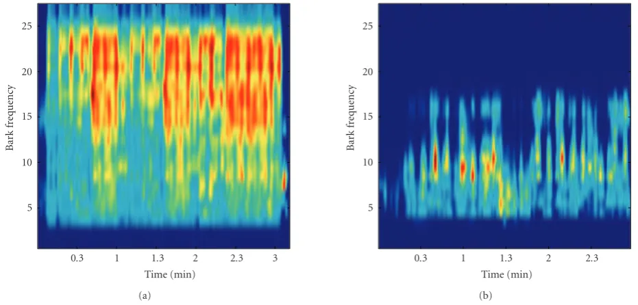
Figure2: Timbregram:PLPcalculated using theGWSof (a)Whenever, Whereverand (b)All of Me.

2.3. Timbre

The timbre is understood here as the spectral estimate and done here using the Gaussian average on the perceptual lin-ear Prediction,PLP [14]. This involves using the bark [18] scale, together with an amplitude scaling that gives an ap-proximation of the human auditory system. ThePLPis cal-culated with a blocksize of approximately 10 milliseconds and with an overlap of 1/2. TheGWSis calculated from the

PLP in steps of 1/2 second, and withσ = 100. This gives a−3 dB width of a little less than one second. A smallerσ

would give too scattered information, while a too large value would smooth thePLPtoo much. An example of thePLPfor the same two songs as above is shown inFigure 2.

The timbregram is just as informative as the rhythmo-gram, although it does not give similar information. While the rhythm evolution is illustrated in therhythmogram, it is the evolution of thetimbre that is shown with the timbre-gram. This includes the insertion of new instruments, such as the trumpet solo in All of Me at approximately 130. The voice is most prominent in thetimbregram. The repeat-ing chorus sections are very visible inWhenever, Wherever, mainly because of the repeating singing style in each chorus, while the choruses are less visible inAll of Me, since it’s sung diﬀerently each time.

2.4. Harmony

The harmony is calculated on an average spectrum, using the Gaussian average, as is the spectral estimate. In this case, the chroma [3] is used as the measure of harmony. Thus, only the relative content of energy in the twelve notes of the octave is found. No information of the octave of the notes is included in thechromagram. It is calculated from theSTFT, using a blocksize of 46 milliseconds. and a stepsize

of 10 milliseconds. The chroma is obtained by summing the energy of all peaks of 12 log₂ of the frequencies hing multiples of 12. By averaghing, ushing the Gaussian av-erage, no specific time localization information is obtained of the individual notes or chords. Instead an estimate of the notes played in the short interval is given as an esti-mate of the scale used in the interval. A step size of 1/2 second is used, together with aσ value of 200, correspond-ing to a −3 dB window of approximately 3 seconds. The

chromagram of the same two songs as above is shown in

Figure 3.

It is obvious that thechromagramshows yet another as-pect of the music. While therhythmogrampinpoints rhyth-mic similarities, and thetimbregram indicates the spectral part of the timbre, thechromagramgives rather precise infor-mation about the chroma of the notes played in the vicinity of the time location. Often, these three aspects of the mu-sic change simultaneously at the segment boundary. Some-times, however, not one of the features can help in, for instance, identifying similar segments. This is the case for the title chorus of All of me, where Billie Holiday and the rhythmic section change the key, the rhythm, and the tim-bre between the first and the second occurrence. Even so, most often, the segment splits are well indicated by any of the features. This is proven in the next section, where first the selfsimilarity of the features are calculated, the segment splits are calculated using a shortest path algorithm with variable segment split cost, and finally these segment splits are matched to manual segment splits of diﬀerent rhythmic music.

2.5. Visualization

Both therhythmogram, thetimbregram, and thechromagram

(5)

0.3 1 1.3 2 2.3 3 Time (min)

C C# D D# E F F#

G G# A A# H

Chr

o

ma

(a)

0.3 1 1.3 2 2.3

Time (min) C

C# D D# E F F# G G# A A# H

Chr

o

ma

(b)

Figure3: Chromagram:chromacalculated using theGWSof (a)Whenever, Whereverand (b)All of Me.

rhythm, timbre, and chroma, as can be seen in Figures1,2, and3. This is believed to be a great help in tasks involving manipulation and analysis of music, for instance for music theorists, DJs, digitalturntablist, and others involved in the understanding and distribution of music.

3. SELF-SIMILARITY

In order to get a better representation of the similarity of the song, a measure of selfsimilarity is used. This was first used in [19] to give evidence of recurrence in dynamic systems. Self similarity calculation is a means of giving evidence of the similarity and dissimilarity of the features. Several stud-ies have used a measure of selfsimilarity [8] in automatic music analysis. Foote [4] used the dot product onmfcc sam-pled at a 100 Hz rate to visualize the selfsimilarity of diﬀerent music excerpt. Bartsch and Wakefield [3] used the chroma-based representation to calculate the cross-correlation and identify repeated segments, corresponding to the chorus, for audio thumbnailing. Later Foote [5] introduced a checker-board kernel correlation as a novelty measure that identifies notes with small time lag, and structure with larger lags with good success. Jensen [7] used smoothed novelty measure to identify structure without the costly calculation of the full checkerboard kernel correlation. In this work, theL2norm is used to calculate the distance between two blocks. The self-similarities ofWhenever, WhereverandAll of Mecalculated for therhythmogram, thetimbregram, and thechromagram

are shown inFigure 4.

It is clear thatWhenever, Wherever contains more sim-ilar music (indicated with a dark color) than All of Me. It has a distinctly diﬀerent intro and outro, and three repeti-tions of the chorus, the third one repeated. While this is vis-ible, in part, in therhythmogram, and quite so in the tim-bregram, it is most prominent in thechromagram, where the

three repetitions of the chorus stand out. As for the intro and the outro, they are quite similar with regard to rhythm, as can be seen in therhythmogram, rather dissimilar with regard to the timbre, and more dissimilar with respect to the chroma-gram. This is explained by the fact that the intro is played on a guitar, the outro on pan-flute, and although they have sim-ilar note durations, the timbres of a pan-flute and a guitar are quite dissimilar, and they do not play the same notes. The situation forAll of Meis that the rhythm is changing all the time, in short segments with a duration of approximately 10 seconds. The saxophone solo at 130 is rather homogenous and similar to the piano intro and some parts of the vocal verse. A large part of the song is more similar with respect to timbre than rhythm or harmony, although most of the song is only similar to itself in short segments of approximately 10 seconds for the timbre, as it is for thechromagram.

4. SHORTEST PATH

Although the segments are visible in the self-similarity plots, there is still a need for a method for identifying the segment splits. Such a method was presented in [13]. In order to seg-ment the music, a model for the cost of one segseg-ment and the segment split is necessary. When this is obtained, the prob-lem is solved using the shortest path algorithm for the di-rected acyclic graph. This method provides the optimum so-lution.

4.1. Cost of one segment

For all features, a sequence 1, 2,. . .,NofN blocks of music is to be divided into a number of segments.c(i,j) is the cost of a segment from blocki to block j, where 1 ≤ i ≤ j ≤

(6)

0.3 1 1.3 2 2.3 3 Duration (min) 0.3

1 1.3 2 2.3 3

Dur

ation

(min)

(a)

0.3 1 1.3 2 2.3 3 Duration (min) 0.3

1 1.3 2 2.3 3

Dur

ation

(min)

(b)

0.3 1 1.3 2 2.3 3 Duration (min) 0.3

1 1.3 2 2.3 3

Dur

ation

(min)

(c)

0.3 1 1.3 2 2.3 3 Duration (min) 0.3

1 1.3 2 2.3 3

Dur

ation

(min)

(d)

0.3 1 1.3 2 2.3 Duration (min) 0.3

1 1.3 2 2.3

Dur

ation

(min)

(e)

0.3 1 1.3 2 2.3 Duration (min) 0.3

1 1.3 2 2.3

Dur

ation

(min)

(f)

Figure4:L2self-similarity for therhythmogram(left),timbregram(middle), andchromagram(right), ofWhenever, Wherever(top) andAll

of me(bottom).

degree of selfsimilarity have a low cost,

c(i,j)=

1

j−i+ 1

j

k=1 k

l=i

Alk. (5)

This cost function computes the sum of the average self-similarity of each block in the segment to all other blocks in the segment. While a normalization by the square of the segment length j−i+ 1 would give the true average, this would severely impede the influence of new segments with larger self-similarity in a large segment, since the large values would be normalized by a relatively large segment length.

4.2. Cost of segment split

Let i1j1,i2j2,. . .,iKjK be a segmentation into K segments, wherei1 =1,i2 = j1+ 1,i3= j2+ 1,. . .,jK =N. The total cost of this segmentation is the sum of segment costs plus an additional cost, which is a fixed cost for a new segment,

E= K

k=1

α+cin,jn

. (6)

By increasingα, the number of resulting segments is de-creased. The appropriate value ofαis found by optimizing the matching of automatic and manual segment splits.

4.3. Shortest path

In order to compute a best possible segmentation, an edge-weighted directed graphG= (V,E) is constructed. The set of nodes isV = 1, 2,. . .,N+ 1. For each possible segment

i j, where 1 ≤ i ≤ j ≤ N, an edge i,j+ 1 exists inE. The weight of the edge i,j + 1 is α+c(i,j). A path inG from node 1 to nodeN+ 1 corresponds to a complete segmenta-tion, where each edge identifies the individual segments. The weight of the path is equal to the total cost of the correspond-ing segmentation. Therefore, a shortest path (or path with minimum total weight) from node 1 to nodeN+ 1 gives a segmentation with minimum total cost. Such a shortest path can be computed in timeO(|V|+|E|)=O(N2_{), since}_G_is acyclic and has|E| = O(N2_{) edges [}₂₀_{]. An illustration of} the directed acyclic graph for a short sequence is shown in

Figure 5.

4.4. Function of split cost

(7)

α+c(1, 2) α+c(2, 3)

α+c(1, 1) α+c(2, 2) α+c(3, 3)

α+c(1, 3)

1 2 3 4

Figure5: Example of a directed acyclic graph with three segments.

increasedα) once the cost of the new segmentation is equal to the original segmentation. The new segmentation cost is now increased withα, until yet another segmentation is cho-sen at equal cost.

Another interesting parameter is the total number of seg-ments. It is plausible that the segmentation system is to be used in a situation where a given number of segments is wanted. This number decreases with the segment cost, as ex-pected. Experiments with a large number of songs show that the number of segments for a givenαis comprised between the half and the double of a median number of segments for most songs.

5. EXPERIMENTS

The segmentation system is now complete. It consists of three different features (therhythmogram,timbregram, and chro-magram), a selfsimilarity measure, and finally the segmenta-tion based on a shortest path algorithm. Two things are inter-esting in the evaluation of the automatic segmentation sys-tem. The first is how the automatic segmentation using the different features actually compare to how humans would segment the music. The second one is whether the diff er-ent features ider-entify the same segmer-entation points. In or-der to test the result, a database on rhythmic music has been collected and manually marked. This database is used here. Three different databases have been segmented manually by three different persons, and segmented automatically using the rhythmic, the timbral, and the harmonic feature. The segmentation points are then matched, and the performance of the segmentation is calculated. No cross-validation has been performed between the subjects.

5.1. Material

Three diﬀerent databases have been collected. One, consist-ing of Chinese music, has been segmented usconsist-ing the Chi-nese numbered notation system [13]. This music consists of 21 randomly selected popular Chinese songs which come from Chinese Mainland, Taiwan, and Hong Kong. They have a variety in tempo, genre, and style, including pop, rock, lyrical, and folk. This music is mainly from 2004. The sec-ond database consists of 13 songs, of mainly electronica and techno, from 2004, and the third database consists of 15 songs, with varying style; alternative rock, ethno pop, pop, and techno. This music is from the 1940s to 2005.

5.2. Manual segmentation

In order to compare the automatic segmentation, the data-bases of music have been manually segmented by three diﬀ er-ent persons. Each database has been segmer-ented by one per-son only. While cross-validation of the manual segmentation could prove useful, the added confusion of the experimental results is believed to confuse the situation. The Chinese pop music was segmented with the aid of a notation system and listening, the other two by listening only. The instructions to the subjects were to try to segment the music according to the assumed structure of popular music, consisting of an intro, chorus, and verse, bridge and outro, with repetitions and omissions, and potentially other segments (solos, vari-ations, etc.). The persons performing the segmentation are professional musicians with a background in jazz and rhyth-mic music. Standard audio editing software was used (Peak and Audacity on Macintosh). For the total database, there is an average of 13 segments per song (first and third quartile are 9 and 17, resp.). The average length of a segment is 20 seconds.

5.3. Matching

The last step in the segmentation is to compare the manual and the automatic segment splits for diﬀerent values of the new segment cost (α). To do this, the automatic segmenta-tions are calculated for increasing values ofα; a low value in-duces many segments, while a high value gives few segments. The manual and automatic segment split positions are now matched, if they are closer than a threshold. For each value ofα, the relative ratios of matched splits to total number of manual splits and to number of automatic splits (recall,R

and precision, P, resp.) are found, and the distance to the optimal result is minimized:

d(α)=1−P(α)2+1−R(α)2. (7) Since this distance is not common in information re-trieval, it is used for matching only here. In the rest of the text, the recall and precision measures, and the weighted sum of these,F1, are used.

(8)

0 1 2 3 4 5 6 7 8 9 10 Matching threshold (s)

0 0.1 0.2 0.3 0.4 0.5 0.6 0.7 0.8 0.9

F1

pe

rf

o

rma

nc

e

Rhythm Timbre Chroma

Figure6: Mean ofF1performance as a function of the matching

threshold for 49 songs.

Table1:F1of the total database for comparison between the

seg-mentation using therhythmogram,timbregram, andchromagram.

Feature Rhythmoghram Timbregram Chromagram

Rhythmoghram 1.00 — —

Timbregram 0.60 1.00 —

Chromagram 0.55 0.60 1.00

It is, therefore, used as the matching threshold in the experi-ments.

5.4. Comparison between features

A priori the rhythmic, timbre, and chroma features should produce approximately the same segmentations. In order to verify this, the distance between the three features has been calculated for all the songs. This has been done for

α = 5.8, 1.3, and 6.2 for rhythm, timbre, and chroma, re-spectively. These are the mean values found in the task of optimizing the automatic splits to the manual splits in the next section. The features generally match well. Only a hand-ful of songs has a perfect match. TheF1performance mea-sure for matching the automatic splits using the three dif-ferent features are shown inTable 1. AnF1value of 0.6 cor-responds approximately to a recall and performance value of between 50–70%. If the comparison between features are done by selecting anαvalue that renders a fixed num-ber of splits (for instance the same numnum-ber as the man-ual segmentation), theF1 value increases approximately by 3%.

This still hides some discrepancies, however, as some songs have rather diﬀerent segmentations for the diﬀ er-ent features. One such example for the first minute ofThe Marriage1 _{is shown in}_{Figure 7}_{. The rhythm only have two}

1_{The Marriage of Hat and Boots}_{by August Engkilde presents Electronic}

Panorama Orchestra (Popscape 2004).

Table2:F1 of the three databases for the segmentation using the

rhythmogram,timbregram, andchromagram.

Database Rhythmoghram Timbregram Chromagram

Chinese pop 0.70 0.75 0.66 Electronica 0.74 0.77 0.66

Varied 0.68 0.74 0.71

Total 0.70 0.75 0.68

Total with fixedα 0.61 0.67 0.56

segment splits (at 13 and 37 seconds) in the first minute, when the bass-rhythm starts and another when the drums join in. The timbre has one additional split at 21 seconds, start of singing, and another, just before one minute. The chroma have the same splits as the timbre, although the split is earlier, at 24 seconds, seemingly because of the slide guitar changing note.

5.5. Comparison with manual segmentation

In this section, the match between the automatic and man-ual segmentations is investigated. For the full database, the rhythm has an average of 10.04 matched splits of 13.39 man-ual (recall = 75%) and of 17.65 automatic splits (preci-sion = 56.9%). F1 = 0.7. The timbre has an average of 10.73 matched splits, of 13.39 manual (recall=80.2%), and 15.96 automatic splits (precision=67.3%).F1 =0.75. The chroma has an average of 10.12 matched splits, of 13.39 man-ual (recall= 75.6%), and 20.59 automatic splits (precision = 49.2%).F1 = 0.68. The Chinese pop database has anF1 values of 0.7, 0.75, and 0.66 for rhythm, timbre, and har-mony, the electronica 0.74, 0.77, and 0.66, while the varied database has 0.68, 0.74, and 0.71. These results can be seen in

Table 2.

These results have been obtained for an optimal alpha value, found using (7). The meanαvalues for each feature are 5.8, 1.3, and 6.2, forrhythm, timbre, and chroma, respec-tively. Theαvalues are rather invariant with respect to the song, with a first and third quartile always between±50%. The meanαis used to separate training and test. The match-ing performance for the automatic segmentation usmatch-ing the meanαcan be seen inTable 2.

The timbre has a better performance in all cases, and it seems that this is the main attribute used when segment-ing music. The rhythm has the next best performance results for the Chinese pop and the electronica, indicating that ei-ther the music is more rhythmically based, or that the per-son performed the manual segmentation based on rhythm, while in the varied database the chroma has the second best performance. All in all, the segmentation identifies most of the manual splits correctly, while keeping the false hits down. The features have comparable results. As the shortest path is the optimum solution, given the error criteria, the perfor-mance errors are a result of either bad features, or errors in the manual segmentation.

(9)

10 20 30 40 50 60 Duration (s)

0.5 1 1.5 2 Rh ythm int er val (s) (a)

10 20 30 40 50 60 Duration (s) 5 10 15 20 25 Bark fr eq ue ncy (b)

10 20 30 40 50 60 Duration (s) C C# D D# E F F# G G# A A# H Chr o ma (c)

10 20 30 40 50 60 Duration (s) 10 20 30 40 50 60 Duratio n (s) (d)

10 20 30 40 50 60 Duration (s) 10 20 30 40 50 60 Duratio n (s) (e)

10 20 30 40 50 60 Duration (s) 10 20 30 40 50 60 Duratio n (s) (f)

Figure7: Rhythm, timbre and chroma ofThe Marriage. Feature (top) and self-similarity (bottom). The automatic segmentation points are marked with vertical solid lines.

0.3 1 1.3 2 2.3 3 Duration (min) 0.2

0.4 0.6 0.8 1 1.2 1.4 1.6 1.8 2 Rh ythm int er val (s)

Automatic segment points Manual segment points

(a)

0.3 1 1.3 2 2.3 3 Duration (min) 5 10 15 20 25 Bark fr eq ue ncy

(b)

0.3 1 1.3 2 2.3 3 Duration (min) C C# D D# E F F# G G# A A# H Chr o ma

(c)

Figure8: (a) Rhythm, (b) timbre, (c) and chroma ofWhenever, Wherever.

55% correspondence between subjects in a free segmentation task, the results are not easily exploitable because of the short sound files (1 minute). However, since manual segmentation seemingly does not perform better than the matching auto-matic and manual splits, it is believed that the results pre-sented here are rather good. Indeed, by manual inspection of the automatic and manual segmentation, the automatic segmentation often makes better sense than the manual one, when conflicting.

As an example of the result, therhythmogram, timbre-gram, and chromagramforWhenever, WhereverandAll of You

are shown in Figures8and9, respectively. The manual seg-mentation is shown in dashed line and the automatic in solid line. The performance forWhenever, WhereverisF1=0.83,

0.81, and 0.8. Good match on all features. All of Me has

F1 =0.48, 0.8, and 0.27. Obviously, in this song, the man-ual segmentation was made on the timbre only, as it has a significantly better matching score.

6. CONCLUSION

(10)

0.3 1 1.3 2 2.3 3 Duration (min) 0.2

0.4 0.6 0.8 1 1.2 1.4 1.6 1.8 2

Rh

ythm

int

er

val

(s)

(a)

0.3 1 1.3 2 2.3 3 Duration (min) 5

10 15 20 25

Bark

fr

eq

ue

ncy

(b)

0.3 1 1.3 2 2.3 3 Duration (min) C

C# D D# E F F# G G#

A A# H

Chr

o

ma

(c)

Figure9: (a) Rhythm, (b) timbre, and (c) chroma ofAll of Me.

are excellent candidates for visualizing the primary attributes of music; rhythm, timbre, and harmony. The songs are seg-mented using a shortest path algorithm based on a model of the cost of one segment and the segment split. The variable cost of the segment split makes it possible to choose the scale of segmentation, either fine, which creates many segments of short length, or coarse, which creates a few long segment. The rhythm, timbre, and chroma create approximately the same number of segments at the same locations in most of the cases. The matching performances (F1), when compared to the manual segmentations are 0.7, 0.75, and 0.68 for rhythm, timbre, and chroma, giving indications that the timbre is the main feature for the task of segmenting music manually. This decreases 10% when separating training and test data, but it is always better than how the automatic segmentation com-pares between features. The automatic segmentation is con-sidered to provide an excellent performance, giving how it is dependent on the music, the person performing the seg-mentation, or the tools used. The features and the segmenta-tion can be used for audio thumbnailing, making a preview, for use in intelligent music scrolling, or in music recomposi-tion.

REFERENCES

[1] T. H. Andersen, “Mixxx: towards novel dj interfaces,” in Pro-ceedings of the International Conference on New Interfaces for

Musical Expression (NIME ’03), pp. 30–35, Montreal, Quebec,

Canada, May 2003.

[2] D. Murphy, “Pattern play,” inAdditional Proceedings of the 2nd

International Conference on Music and Artificial Intelligence, A.

Smaill, Ed., Edinburgh, Scotland, September 2002.

[3] M. A. Bartsch and G. H. Wakefield, “To catch a chorus: us-ing chroma-based representations for audio thumbnailus-ing,” in

Proceedings of IEEE Workshop on Applications of Signal

Process-ing to Audio and Acoustics, pp. 15–18, New Paltz, NY, USA,

October 2001.

[4] J. Foote, “Visualizing music and audio using self-similarity,”

in Proceedings of the 7th ACM International Multimedia

Conference & Exhibition, pp. 77–80, Orlando, Fla, USA,

November 1999.

[5] J. Foote, “Automatic audio segmentation using a measure of audio novelty,” inProceedings of IEEE International Conference

on Multimedia and Expo (ICME ’00), vol. 1, pp. 452–455, New

York, NY, USA, July-August 2000.

[6] M. Cooper and J. Foote, “Summarizing popular music via structural similarity analysis,” in Proceedings of IEEE Work-shop on Applications of Signal Processing to Audio and

Acous-tics (WASPAA ’03), pp. 127–130, New Paltz, NY, USA, October

2003.

[7] K. Jensen, “A causal rhythm grouping,” inProceedings of 2nd International Symposium on Computer Music Modeling and

Re-trieval (CMMR ’04), vol. 3310 ofLecture Notes in Computer

Science, pp. 83–95, 2005.

[8] G. Peeters and X. Rodet, “Signal-based music structure dis-covery for music audio summary generation,” inProceedings

of International Computer Music Conference (ICMC ’03), pp.

15–22, Singapore, Octobre 2003.

[9] R. B. Dannenberg and N. Hu, “Pattern discovery techniques for music audio,”Journal of New Music Research, vol. 32, no. 2, pp. 153–163, 2003.

[10] M. Goto, “A chorus-section detecting method for musical au-dio signals,” inProceedings of IEEE International Conference on

Acoustics, Speech and Signal Processing (ICASSP ’03), vol. 5, pp.

437–440, Hong Kong, April 2003.

[11] S. Dubnov, G. Assayag, and R. El-Yaniv, “Universal classifica-tion applied to musical sequences,” inProceedings of the

Inter-national Computer Music Conference (ICMC ’98), pp. 332–340,

Ann Arbor, Mich, USA, October 1998.

[12] T. Jehan, “Hierarchical multi-class self similarities,” in Proceed-ings of IEEE Workshop on Applications of Signal Processing to

Audio and Acoustics (WASPAA ’05), pp. 311–314, New Paltz,

NY, USA, October 2005.

[13] K. Jensen, J. Xu, and M. Zachariasen, “Rhythm-based segmen-tation of popular chinese music,” inProceedings of 6th

Interna-tional Conference on Music Information Retrieval (ISMIR ’05),

pp. 374–380, London, UK, September 2005.

(11)

[15] K. Jensen, “Perceptual atomic noise,” inProceedings of the

In-ternational Computer Music Conference (ICMC ’05), pp. 668–

671, Barcelona, Spain, September 2005.

[16] N. Collins, “A comparison of sound onset detection algo-rithms with emphasis on psychoacoustically motivated de-tection functions,” inProceedings of AES 118th Convention, Barcelona, Spain, May 2005.

[17] P. Desain, “A (de)composable theory of rhythm,”Music

Per-ception, vol. 9, no. 4, pp. 439–454, 1992.

[18] A. Sekey and B. A. Hanson, “Improved 1-bark bandwidth auditory filter,”Journal of the Acoustical Society of America, vol. 75, no. 6, pp. 1902–1904, 1984.

[19] J. P. Eckmann, S. O. Kamphorst, and D. Ruelle, “Recurrence plots of dynamical systems,”Europhysics Letters, vol. 4, no. 9, pp. 973–977, 1987.

[20] T. H. Cormen, C. Stein, R. L. Rivest, and C. E. Leiserson,

Introduction to Algorithms, The MIT Press, Cambridge, UK;

McGraw-Hill, New York, NY, USA, 2nd edition, 2001. [21] G. Tzanetakis and P. Cook, “Multifeature audio segmentation

for browsing and annotation,” inProceedings of the IEEE Work-shop on Applications of Signal Processing to Audio and

Acous-tics (WASPAA ’99), pp. 103–106, New Paltz, NY, USA, October

1999.

Kristoﬀer Jensenobtained his Masters de-gree in 1988 in computer science from the Technical University of Lund, Sweden, and a D.E.A in signal processing in 1989 from the ENSEEIHT, Toulouse, France. His Ph.D. was delivered and defended in 1999 at the Department of Computer Science, Uni-versity of Copenhagen, Denmark, treating signal processing applied to music with a physical and perceptual point of view. This