Volume 2010, Article ID 167942,12pages doi:10.1155/2010/167942
Research Article
A Conditional Random Field Approach to Unsupervised Texture
Image Segmentation
Chang-Tsun Li
Department of Computer Science, University of Warwick, Coventry CV4 7AL, UK
Correspondence should be addressed to Chang-Tsun Li,[email protected]
Received 6 June 2010; Revised 16 August 2010; Accepted 10 September 2010
Academic Editor: Stephen Marshall
Copyright © 2010 Chang-Tsun Li. This is an open access article distributed under the Creative Commons Attribution License, which permits unrestricted use, distribution, and reproduction in any medium, provided the original work is properly cited.
An unsupervised multiresolution conditional random field (CRF) approach to texture segmentation problems is introduced. This approach involves local and long-range information in the CRF neighbourhood to determine the classes of image blocks. Like most Markov random field (MRF) approaches, the proposed method treats the image as an array of random variables and attempts to assign an optimal class label to each. While most MRFs involve only local information extracted from a small neighbourhood, our method also allows a few long-range blocks to be involved in the labelling process. This alleviates the problem of assigning different class labels to disjoint regions of the same texture and oversegmentation due to the lack of long-range interaction among the neighbouring and distant blocks. The proposed method requires noa prioriknowledge of the number and types of regions/textures.
1. Introduction
Image segmentation is essentially the first step toward many image analysis and computer vision problems. It is usually formulated as an optimization problem, in which the image in question is partitioned into a number of homogeneous regions, each characterized by a unique set of features [1]. Its applications can be found in a wide variety of areas, such as biomedical image processing [2–4], remote sensing [5– 7], target identification and tracking [8], anomaly detection [9], video analysis [10], scene segmentation [11,12], sonar imagery [13], surveillance [14], land use [15–17], and image database retrieval [14, 18]. However, segmenting textured images is not a trivial task for various reasons.
(i) Firstly, textures comprise primitives/textons and tiny edges (intensity fluctuations), which can cause false responses in conventional edge detectors, while tex-ture boundaries do not appear as conventional edges and therefore often go undetected by conventional edge detectors.
(ii) Secondly, another major difficulty in texture segmen-tation arises from the fact that texture is a regional property [19] rather than a pixel property. The
information in a single pixel is only the intensity or colour. By contrast, we need to cover a reasonably large area of pixels in order to extract meaningful texture features. If we take a big area of a textured image into consideration, we get high confidence in the class of the texture. However, we lose the resolution in which the texture boundary may be if the area in question contains more than one class of textures. On the other hand, if we confine the analysis to a smaller area, the confidence in the position of texture boundaries increases at the expense of the certainty of texture class. This phenomenon, known as “class-boundary uncertainty” [1], suggests that information at multiple resolutions or scales has to be fused in some way for effective segmentation. This motivates the adoption of the various multiresolution approaches in many works [20–23].
of textures contained in the target image [1]. The latter means that it is preferable not to have a training phase before the algorithm is used. This requirement is sensible because if the training phase were needed, then when textures outside the training set appear in the images to be segmented, the algorithm would have difficulty identifying them.
(iv) Moreover, an intelligent algorithm should not only be able to segment images into regions, but also be capable of classifying disjoint regions of the same texture into the same class [15, 16]. For example, an algorithm capable of segmenting an aerial image with two disjoint urban areas from their woodland background and assigning the same class label to the two urban areas is certainly superior to an algorithm only capable of segmenting the image into three regions.
The motivation of this work is to develop an unsu-pervised algorithm, which is capable of meeting these requirements.
2. Related Work
In the last few decades, a wide variety of methods, such as fuzzy clustering [19, 23], watershed transform [18], active contours [24], independent component analysis [25], and morphology-based estimation [26], have been explored to solve the problem of texture segmentation. Among them, Markov random field (MRF) [1, 7, 9, 27, 28] is one of the most frequently used approaches due to the simplicity of its local characteristics (also known as Markovianity) [29]. Markovianity allows a global optimization problem to be solved locally and this is confirmed by the results reported in our recent work [1]. The approach presented in [1] is a typical combination of MRFs and simulated annealing, known as the Gibbs sampler [21]. The idea is to divide an image into a number of blocks and treat each block as a random variable to be assigned a class label depending on its own features, its neighbours’ features, and class labels. When a block b is visited, the probabilities of the labels assigned to its neighbours are calculated according to a cost function. The optimal label is assigned the highest probability and the less promising labels get lower probabilities. Simulated annealing [21] is then applied so as to assign one of the labels to block b. When the labelling process converges, the labelling result is propagated down to the next resolution level for finer segmentation. This process is repeated until a nominal bottom level is reached. Since this is a multiresolution approach, the neighbourhood includes the 4 neighbours at the same level and the parent block at one level above (except the nominal top level). By using the idea of SOIL(set of indispensable labels) reported in [30] and exploitinglocal feature disparities, this work requires no
a prioriglobal knowledge about the number of texture classes and the types of textures contained in the images. However, the work has the following limitations.
(i) Due to the lack of long range interaction with blocks outside the local neighbourhood and the fact that the algorithm starts with a random class label configuration, disjoint regions of the same texture are assigned different class labels. An example is shown in Figure 1(a), wherein the two disjoint regions on the right and left sides containing the same texture have been misclassified into two different classes—class 5 and 7, as shown inFigure 1(b).
(ii) Again, for the same reason, large or elongated regions may be oversegmented. For example, the region in the middle of Figure 1(a) has been oversegmented into two classes with labels 2 and 9, as shown in Figure 1(b). This can be explained as follows. Given Figure 1(b) as the current label configuration, with a 4-neighbourhood system, despite the fact that sites (5, 5) and (6, 5) belong to the same region, when site (5, 5) is visited, three of its neighbours within the 4-neighbourhood system are labelled 2 while only one is labelled 9. Therefore, the probability of assigning 2 to site (5, 5) is high, while the probability of assigning label 9 will decrease as relaxation proceeds. Similarly, site (6, 5) is next to three neighbours with label 9 and only one with label 2. Therefore the probability that it will be assigned label 9 is far greater than getting assigned label 2. This kind of local “sibling competition” can lead to premature convergence at local minima in the energy landscape and conse-quently give rise to oversegmentation. This type of oversegmentations is more likely to occur in large or elongated regions, where different class labels may grow into subregions from different locations of the regions. When these subregions meet, sibling compe-tition starts and spurious boundaries may form. (iii) The energy function adopted in [1] was based on the
assumption that the distributions of both intraclass and interclass feature disparities of useful features are approximately Gaussian. Although this is a reasonable assumption, the accuracy of the prior model may have significant influence on the efficacy of the segmentation. The potential function, which is encoded in the energy function, is also complicated and needs to be recalculated iteratively in an iterated conditional mode (ICM) sense [29].
(a)
1 2 3 4 5 6 7 8
1 5 5 2 2 2 2 7 7
2 5 5 2 2 2 2 7 7
3 5 5 2 2 2 2 7 7
4 5 5 2 2 2 2 7 7
5 5 5 2 2 2 2 7 7
6 5 5 9 9 9 9 7 7
7 5 5 9 9 9 9 7 7
8 5 5 9 9 9 9 7 7
i j
(b)
Figure1: (a) A textured image. (b) A possible label configuration with the numbers representing the class labels.
As described in the next section, we propose an improved Markov random field (MRF) approach, which involves both local and long-range information in a simpler energy function, to alleviate the aforementioned limitations of our previous work [1]. The objectives of the proposed work are as follows:
(i) resolving local sibling competition in order to tackle the problem of oversegmentation,
(ii) labelling disjoint regions of the same texture con-sistently by involving long-range interaction among blocks,
(iii) reducing the computational cost by simplifying the energy function and facilitating information fusion through long range interaction among blocks.
3. Multiresolution Markov Random Field
Texture Segmentation Algorithm
To avoid confusing the reader with details, we first present the whole picture of the proposed algorithm as follows.
Multiresolution Conditional Random Field Texture Segmenta-tion Algorithm
(1) Build a multiresolution pyramid conforming to a quad-tree structure.
(2) Extract texture features from each image block. (3) Assign a random label to each block at the top level
to form an initial label configuration.
(4) For each resolution level before the nominal bottom level is reached
(4.1) While not converged, for each block (4.1.1) form a voting pool,
(4.1.2) calculate the energy functions of the labels of the members in the voting pool, (4.1.3) calculate the probabilities of the labels
based on their energy functions,
(4.1.4) assign one of the labels according the probability,
(4.2) propagate results to the next resolution level.
In the first step of the proposed algorithm, a multireso-lution framework is adopted to represent the image data at multiple scales in order to alleviate the canonical problem of class-boundary uncertainty [1,2]. Note that in order not to complicate the symbols in the presentation of the algorithm later, we will assume that the original images are square. However, the two dimensions of the original image need not to be equal. We create an image pyramid conforming to a quad-tree structure withLresolution levels based on the original image of 2L×2Lpixels. Each levellconsists of an array of 2l×2l sites/blocksof 2L−l×2L−lpixels by sliding a window of 2L−l×2L−lpixels over the original image in 2L−l−1
-pixel wide steps in both horizontal and vertical directions. That is to say that the sampling windows are 50% overlapped. At the higher levels, the size of the block is larger, which gives higher resolution of texture classes but lower resolution of texture boundaries. While at lower levels, the blocks are smaller, and as a result, higher boundary resolution is gained at the expense of class resolution. At the top level (i.e.,l =
0), there is only one block, which covers the whole image; therefore, the algorithm must start at a nominal top level l > 0 in order to carry out the segmentation task. At the bottom level (i.e.,l =L), each block covers only one pixel, which carries no texture features. Therefore, the algorithm should stop at a nominal bottom level withl < L.
Usually a complete segmentation process includes a
feature extractionstage, followed by alabellingstage. At the first step of the proposed algorithm, a set of texture features is extracted from each site b as the observed data Yb. In practice, features suitable for the segmentation task are image and application dependent. Since the main purpose of this work is to propose, not a feature extraction method, but a generic labelling algorithm, we include only the mean and variance of the intensity in the feature set. However, the reader is reminded that appropriate features other than mean intensity and variance can be incorporated with the proposed labelling algorithm since the feature extraction and labelling processes are separate modules.
2 2 2 6 7 7 7 7
1 2 2 6 7 7 7 7
1 1 1 7 7 7 7 7
1 1 1 7 7 7 5 7
1 1 1 7 7 7 7 7
1 1 1 4 7 7 7 7
1 1 3 3 7 7 7 7
1 1 3 3 3 7 7 7
1
(a) Label configuration at levell
1 1 7 7
1 1 7 7
1 1 7 7
1 1 7 7
(b) Label configuration at levell−1
Figure2: Voting pool of site (5, 3, l), the grey block in (a), at resolution levell. The voting pool consists of the sites highlighted with bold line segments in both (a) and (b), which includes parent site (3, 2, l −1) at levell−1 in (b), 4 neighbours at (4, 3, l), (5, 4, l), (6, 3,l), (5, 2, l), two randomly picked sites at (8, 3, l) and (6, 8, l), and themost differentsite at (5, 6,l).
Xb. The task of the segmentation algorithm is to assign an optimal class labelxb (an instance of the random variable) to each siteb, depending on the observed dataYb atb, the observed dataYrand class labelsXr, for all sitesrin a “voting pool”, Nb. This can be formulated as a random field (RF) model according to the Bayes theorem
PXb=xbYb=yb,YNb=yNb,XNb=xNb
,
∝PYb=yb,YNb=yNb|Xb=xb,XNb=xNb
×PXb=xbXNb=xNb
,
(1)
where YNb(yNb) and XNb(xNb) represent the observed data and class labels of all the sitesr inNb, respectively. That is, YNb = {Yr | r ∈ Nb}andXNb = {Xr | r ∈ Nb}.P(Yb = yb,YNb =yNb |Xb=xb,XNb =xNb) andP(Xb=xb |XNb = xNb) are the conditional probability distribution and prior probability distribution, respectively. Usually, the number of texture classes in the image in question is unknown to the user. To allow the algorithm to work without the user specifying the number of texture classes, at the nominal top level, each block is assigned a label randomly picked from the integer range [1, M], whereMis the number of blocks at the nominal top level. That is, we allow the algorithm to start with a completely random label configuration. This is virtually equivalent to adopting an “infinite” label space.
The neighbourhood system of MRF algorithms plays an important role in the segmentation process. As mentioned in the previous section, the lack of long-range interaction during the labelling processing in the algorithm of [1] is the key reason that oversegmentation occurs and that the algorithm is not able to assign the same class label to disjoint regions of the same texture; it is also one of the reasons why the algorithm’s convergence rate cannot be accelerated. To involve long-range interaction, when a sitebat levellis being visited, in addition to itsparentblockpat levell−1 and the
4 neighbours(n1,n2,n3, andn4) at levell, three other blocks,
r1,r2, andrdare also included in the voting poolNb.r1and
r2are selected at random, andrdis the block whose feature
set is most different from that ofb. So, the voting pool can be expressed as
Nb=
p,n1,n2,n3,n4,r1,r2,rd
. (2)
For example, let (i,j,l) denote a site appearing at coordinates (i,j) at levell. Figure 2demonstrates that the voting pool of site b at (5, 3,l) is Nb = {p,n1,n2,n3,n4,r1,r2,rd} =
{(3, 2,l−1), (4, 3,l), (5, 4,l), (6, 3,l), (5, 2,l), (8, 3,l), (6, 8,l), (5, 6,l)}, where (3, 2,l−1) is to be found inFigure 2(b), while others are to be found inFigure 2(a). Apart from the parent block and the 4 neighbours, all the other members may be different in different iterations. Themost differentblock,rd, is the one identified from the randomly picked members during the whole labelling history. That is, in any iteration, if a voting block selected at random (i.e.,r1or r2) is more
different from b than the current most different block, the
most different block is replaced by that voting block. Note that at the top resolution level, there is no parent block in the voting pool. In addition to playing the same role asr1 and
r2 of introducing long-range interaction, the most different
blockrd plays an extra role of informing the algorithm that the label associated with the most different block is to be avoided. Because of the contextual property of texture, there is no need to keep track of the most similar block for each siteb, given the fact that the 4 neighbours have already been included in the voting pool.
diversity by sampling the label configuration of the whole image from a virtually infinite label space. Secondly, the computational cost is kept low because locally the optimal label of each individual block is sampled from a small space with its cardinality≤8 because there are at most 8 members in the voting pool Nb. The cardinality of Nb will decrease in due course as the homogeneous regions emerge. In our previous example, the cardinality is only 3. Although starting from a random initial label configuration, a unique optimal label for each texture class can be quickly identified through the interaction with the members of the voting pool. It should be noted that, at lower resolution levels, a random label that is not assigned to any site can be included as a candidate in order to encourage small regions to emerge. However, texture class certainty is lower at lower resolution levels and texture may comprise recursive patterns/textons, which can be smaller than the image blocks. Including such an unused label increases the possibility of detecting small spurious regions that are actually part of a larger and genuine texture region. Therefore, whether to include such a label as candidate is application dependent. In this work, we choose not to include it.
The conditional random field (CRF) model of (1) can also be expressed in Gibbs form [21] in terms of energy functionsUbc(yb,yNb | xb,xNb) andU
p
b(xb |xNb) within the voting poolNbas
Pxb|yb,yNb,xNb
∝ 1
Zb
exp−Uc b
yb,yNbxb,xNb
−Ubp
xb|xNb
, (3)
whereUc
b(yb,yNb | xb,xNb) andU p
b(xb | xNb) are associated with the conditional probability distribution and prior probability distribution of (1), respectively, and Zb is the so-called partition function, which is to serve the purpose of normalisation. By properly reformulating the two energy functions in (3), as described in [21], we obtain a new model as
Pxbyb,yNb,xNb
= 1
Zb
exp−Ub
yb,yNb,xb,xNb , (4)
where the partition function is
Zb=
xb∈xNb
exp−Ub
yb,yNb,xb,xNb . (5)
Like most optimisation processes, defining a feasible objective function is important, yet by no means trivial. In the proposed algorithm, the energy functionUb is defined as the sum of the pairwise potentialsVb,rbetween siteband voting membersrinNb:
Ub
yb,yNb,xb,xNb
=
r∈Nb Vb,r
yb,yr,xb,xr
, (6)
where the potentialVb,ris defined as
Vb,r
yb,yr,xb,xr
=
⎧ ⎨ ⎩
−D−db,r
ifxb=xr, D−db,r ifxb=/xr,
(7)
where db,r is the feature disparity between sites b and r, defined as
db,r = yb−yr (8)
andDis the estimatedthresholddividing the space offeature disparities into subspaces of intra- and interclass feature disparities. To estimateDfor each resolution level, 300 pairs of blocks are picked at random from the same resolution level and theirfeature disparitiesare calculated. We allow a block to be paired with more than one partner. Since some pairs might belong to the same texture class and some might not, we can have two types of feature disparity:intraclass with relatively smaller value andinterclasswith relatively greater value.By taking the smallest and the greatest feature disparity as the initial centroids ofintraclassandinterclass,respectively, a trivial 2-mean clustering method is employed to partition the space of the 300 feature disparities into two clusters. Then,Dof (5) can be calculated according to
D=1
2(dw+do), (9)
where dw is the greatest value in intraclass and do is the smallest value in interclass. The feasibility of the energy function Ub and pairwise potential Vb,r is discussed as follows.
(i) The first merit is that D, db,r, dw, and do are all adaptive to the content of the image. Since the complexity of (5) is low, the computational cost of calculating the energy function defined in (4) is significantly lower than the one used in [1].
(ii) In the approach reported in [19,21,22], the potential function is defined as
Vb,r
yb,yr,xb,xr
=
⎧ ⎨ ⎩
−β ifxb=xr β ifxb=/xr,
(10)
(iii) Assuming the texture features employed are ade-quately discriminative, then
(a) the first case of (7) indicates that if the same
class labelxris to be assigned to siteb, then, (1) if blockbandr dobelong to the same class
(i.e.,db,ris significantlysmallerthanD), a
smallvalue,−(D−db,r), for potentialVb,r is given. This is reasonable because this is a correct labelling and should be encouraged with a lower cost,
(2) if blockbandrdonotbelong to the same class (i.e.,db,r is significantlygreaterthan D), alargevalue,−(D−db,r), for potential
Vb,rwill be given as a penalty to discourage this incorrect labelling;
(b) the second case of (5) indicates that if a class labeldifferentfromxris to be assigned to siteb, then,
(1) if blockbandr dobelong to the same class, alargevalue, (D−db,r), for potentialVb,ris given to penalise this incorrect labelling, (2) if blockbandrdonotbelong to the same
class, asmallvalue, (D−db,r), for potential
Vb,rwill be given to encourage this correct labelling.
In optimization problems, deterministic relaxation [22] and stochastic relaxation [1,21] are two common techniques for selecting next states based on the objective function associated with the current states and the observed data. In the context of this work, given the energy function (the objective function), a sitebcan be assigned a class label in a deterministic sense according to (11)
xb=arg max k P
Xb=k yb,yNb,xNb
, (11)
whereP(·) is defined in (4).
Although deterministic relaxation is relatively less com-putationally intensive compared to stochastic relaxation, a main limitation is that the relaxation process may get trapped in local optimal states more easily. Therefore, in this work we choose stochastic relaxation, which combines simulated annealing (SA) [1,21] with the MRF model of (4), to select an optimal label from the ones associated with the members of the voting pool for site b. With this stochastic sense, a modified model of (4) is defined as
Pxsyb,yNb,xNb
=exp
−Ub
yb,yNb,xb,xNb
T(i,l)
, (12)
where T(i,l) in (12) is the pseudotemperature (also called
annealing schedule) in iterationiat resolution levell
T(i,l)= C(l)
log(1 +i), (13)
whereC(l) in (13) is a constant which determines the initial temperature and the convergence rate. The higher the value
ofC(l) is, the higher the starting pseudotemperature is and the less likely the labelling process will get trapped at local minima, but the slower the convergence rate is. Because the labelling at low resolution levels is conditioned on the segmentation result of the higher resolution levels, wherein the number of blocks is smaller,C(l) is varied withl, with greater values at low l (high resolution level). Usually, the value ofC(l) has to be chosen empirically according to the range of the energy function. Note that in the special case when T(i,l) is fixed at 0 regardless i and l, the stochastic model of (12) is equivalent to the deterministic model as expressed in (11).
The search for the optimal label xb is the process of maximizing the a posteriori probability of (12). In the context of simulated annealing and stochastic relaxation, the label of each voting member has a chance of being chosen proportional to its probability calculated according to (12).
The algorithm can certainly involve only one or more than two random sites. There is no theoretical backing for determining the number of random sites as this is application dependent. For example, when segmenting images with disjoint small regions of the same texture, the inclusion of more random sites increases the chances for the disjoint small regions to establish contact. However, this is achieved at the expense of computation complexity because there will be more sites and more labels to deal with. On the other hand, when segmenting images without disjoint small regions of the same class, the inclusion of less random sites is more desirable. Nonetheless, the word “small” in this context is not well defined, and maybe there is no way of defining it. Moreover, this question about how many random sites are enough is also directly related to the setting of the starting temperature for simulated annealing. With the number of random sites fixed, when the starting temperature is set high, the algorithm will iterate longer, allowing more sites to be interacted with. So, like the starting temperature, the number of random sites has to be determined in an ad hoc manner. In this work, given the small number of the standing members (i.e., 4 first-order neighbours), including half as many random sites is a reasonable guess.
As stated in Step (4.2), upon convergence, the algorithm propagates the segmentation result of the current level down to the next level for refinement. The propagated result is the class label configuration, which will be used as the initial configuration at the new level.
4. Experiments and Performance Analyses
Table1: Performance in terms of computational cost measured by average iterations, oversegmentation rate, and rate of differently labelling disjoint regions of the same texture (%) with various values ofCwhen the image inFigure 3is divided into 64 blocks.
C Average iterations Oversegmentation rate (%) Rate of labelling disjoint regions differently (%)
Proposed alg. Previous alg. Proposed alg. Previous alg. Proposed alg. Previous alg.
10 5.9 6.9 1 100 1 100
50 6.2 10.6 0 100 0 100
100 7.2 23.8 0 91 0 100
200 9.4 32.3 0 22 0 99
300 12.7 46.1 0 3 0 96
400 19.28 72.1 0 2 0 86
500 28.4 131.3 0 0 0 55
600 38.8 218.2 0 0 0 51
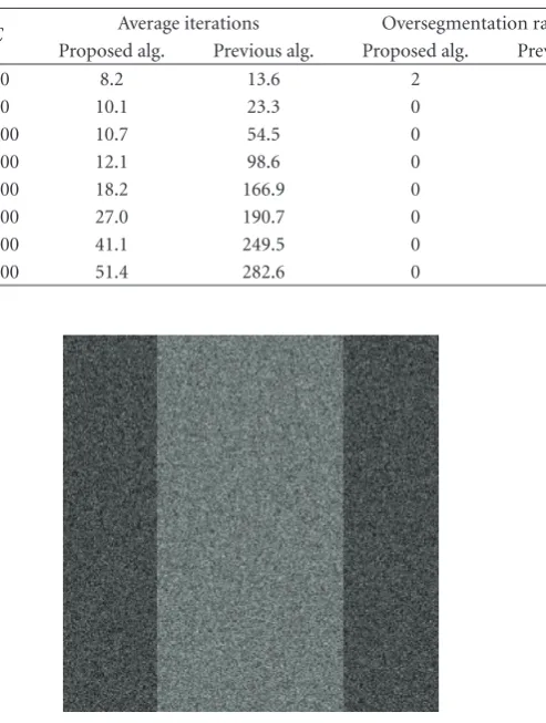
Table2: Performance in terms of computational cost measured by average iterations, oversegmentation rate, and rate of differently labelling disjoint regions of the same texture (%) with various values ofCwhen the image inFigure 3is divided into 256 blocks.
C Average iterations Oversegmentation rate (%) Rate of labelling disjoint regions differently (%)
Proposed alg. Previous alg. Proposed alg. Previous alg. Proposed alg. Previous alg.
10 8.2 13.6 2 100 1 100
50 10.1 23.3 0 100 0 100
100 10.7 54.5 0 100 0 100
200 12.1 98.6 0 100 0 100
300 18.2 166.9 0 91 0 100
400 27.0 190.7 0 34 0 100
500 41.1 249.5 0 11 0 100
600 51.4 282.6 0 0 0 100
Figure3: Test image containing two disjoint darker regions with a mean equal to 80 and variance equal to 100 separated by another brighter region with a mean equal to 100 and variance equal to 100.
so that even the variation of the features extracted from small blocks of the same region is small. This means that the performance we want to evaluate is not biased by the features. We apply the proposed algorithm and the previous one reported in [1] 100 times each to segment the image. To compare the performance on equal basis, we allow both algorithms to use the same energy function defined in (6). Table 1differently shows the two algorithms’ performance in
terms of computational cost measured byaverage iterations, oversegmentation rate, and rate of labelling disjoint regions of the same texture when the image in Figure 3is divided into 64 blocks. Table 2 lists the same measurements of the two algorithms’ performance when the same image is divided into 256 blocks. The average iterations in Table 1 indicate that the proposed algorithm is significantly more efficient in terms of computational cost than the previous algorithm even without taking the other two metrics of performance into account. They also indicate that the pro-posed algorithm’s computational cost increases significantly more slowly than that of the previous algorithm. Moreover, we can see that at C = 10, only 1% of the applications of the proposed algorithm result in oversegmentation and labelling of the two dark regions differently, due to the low initial annealing temperature, while no oversegmentation and mislabelling of the dark regions occur whenC is only 50, with an average computational cost of only 6.2 iterations. On the contrary, the previous algorithm could only yield no oversegmentation when C = 500, with the average computational cost as high as 131.3 iterations. The rates of labelling the two dark regions inconsistently associated with the proposed and previous algorithms also reveal another superior aspect of the proposed algorithm. As we mentioned earlier, the larger the textured regions are, the higher the probability that the previous algorithm will encounter the problem of oversegmentation.
(a) (b)
(c) (d)
Figure4: Segmentation results ofImage Iat 3 different resolution levels.
4 times more blocks, the proposed algorithm demonstrates the same level of performance, in terms of oversegmentation rate and rate of labelling the two dark regions differently, with a slight increase of computational cost compared to Table 1. For the previous algorithm, the computational cost increases more significantly (with an average computational cost of 282.6 iterations) and the initial temperature has to be set to 600 in order to avoid oversegmentation. On the other hand, the proposed algorithm is able to achieve this level of performance with C = 50 and an average cost of 10.1 iterations. Nevertheless, in all cases, as demonstrated in Table 2, the previous algorithm completely fails to label the two dark regions consistently. These two experiments demonstrate that the voting pool adopted in the proposed algorithm can effectively and efficiently facilitate both local and global interactions among the blocks to avoid the key limitations of the previous algorithm.
Figures 4, 5, and 6 illustrate the segmentation results of three textured images, Image I, II, and III, at different resolution levels. This time the previous algorithm uses the energy function defined in [1] while the proposed algorithm uses the one adopted in this work. The value ofCin (13) is
set to 300 at the nominal top resolution level and reduced by 50 after proceeding to the next resolution level. The results are shown in (a) to (d) of Figures 4to6, respectively. The results show the increase in segmentation accuracy and the algorithm’s ability to alleviate theclass-boundary uncertainty
(a) (b)
(c) (d)
Figure5: Segmentation results ofImage IIat 3 different resolution levels.
previous algorithm came with a boundary process. Although the boundary process made the boundaries look smoother, it did not provide significant improvement in terms of segmentation accuracy. Therefore, we do not include the boundary process in this work. Note, in all the experiments, no a priori knowledge about the number and types of textures contained in the images in question is provided to the algorithm. Yet, the algorithm is able to segment the images correctly. These results indicate that the proposed algorithm requires no supervision by the user.
It is also worth noting that, in Figure 4, the ele-ments/textons of the recursive texture pattern are greater than 16 pixels in at least one dimension, which is greater than the block dimension at the resolution level 5. Yet the proposed algorithm is capable of detecting the boundaries accurately even at the bottom level, where the block size is only 8×8 pixels. This is due to the use of multiresolution approach: we divide the images into large blocks at the top level to collect reliable features (at the expense of boundary certainty) and use the coarse segmentation result to condition the segmentation at lower level.
Table3: Comparisons of performance in terms of segmentation error rates and computational cost measured by number of iteration per pixels (# i/p) for ImageIofFigure 4.
Levell
Segmentation error rate (%) # i/p Proposed
alg.
Previous alg.
Proposed alg.
Previous alg.
3 3.145 7.053 0.012 0.189
4 1.836 1.640 0.027 0.074
5 1.176 1.265 0.250 0.349
0.587 0.716 0.375 2.191
Total # i/p 2.803
(a) (b)
(c) (d)
Figure6: Segmentation results ofImage IIIat 3 different resolution levels.
Table4: Comparisons of performance in terms of segmentation error rates and computational cost measured by number of iteration per pixels (# i/p) for ImageIIofFigure 5.
Levell
Segmentation error rate (%) # i/p Proposed
alg.
Previous alg.
Proposed alg.
Previous alg.
3 2.780 6.953 0.014 0.186
4 1.663 1.807 0.027 0.066
5 1.160 1.035 0.250 0.531
6 0.812 0.848 0.375 2.499
Total # i/p 3.282
resolution level 3 (i.e., block size = 64 ×64), but only demonstrate the segmentation results at level 4 to 6 in Figures 7(b)–7(d), respectively. This experiment conforms to what we mentioned inSection 3that the proposed segmentation algorithm can be incorporated with any discriminative features. The key challenges posed by this image are the following. (1) The feature difference between the leaves
Table5: Comparisons of performance in terms of segmentation error rates and computational cost measured by number of iteration per pixels (# i/p) for ImageIIIofFigure 6.
Levell
Segmentation error rate (%) # i/p Proposed
alg.
Previous alg.
Proposed alg.
Previous alg.
3 6.137 6.892 0.011 0.202
4 3.772 5.852 0.023 0.125
5 2.264 3.603 0.250 0.594
6 1.245 2.237 0.375 2.237
Total # i/p 3.541
(a) original image (b) level 4
(c) level 5 (d) level 6
Figure7: Segmentation results ofOrchidat 3 different resolution levels.
0 20 40 60 80
200 150
100 50
0 0 50
100 150
200 250
Figure8: Colour distribution of 2400 blocks of 8×8 pixels taken fromFigure 7(a). The data points in the circle closer to the origin correspond to the dark background ofFigure 7(a)while the points in the other circle correspond to the leaves. The uncircled cluster corresponds to the flower region.
into the same group. (2) The left part of the flower shape is quite rugged. (3) There are two narrow orange “peninsulas”, one pointing upwards and the other downwards. It can be seen from Figure 7(b) that, because of class-boundary uncertainty, many spurious small regions form along the boundaries between real regions, the rugged boundaries and the two peninsulas in particular. The sizes of the small regions can be reduced at finer resolution levels, but the number of even smaller regions will also increase at finer resolution levels. These small regions are inherent to the class-boundary uncertainty. Their areas are less significant at
finer resolution levels, and segmentation inaccuracy at higher resolution levels can be reduced at finer levels; therefore, it is computationally undesirable to repeat the same algorithm at finer levels with the same sophistication. To keep computa-tional cost low without sacrificing segmentation accuracy, at the two finest resolution levels, we apply the algorithm with stochastic relaxation (12) to all the blocks for three iterations and then only to blocks with at least one 4-neighbour system carrying a different class label (i.e., the blocks along the boundaries) in a deterministic relaxation manner (11).
5. Conclusions
In this work, we have addressed the need for tackling the
References
[1] R. Wilson and C.-T. Li, “A class of discrete multiresolution random fields and its application to image segmentation,”
IEEE Transactions on Pattern Analysis and Machine Intelligence, vol. 25, no. 1, pp. 42–56, 2003.
[2] C. C. R. Aldasoro and A. Bhalerao, “Volumetric texture segmentation by discriminant feature selection and multires-olution classification,”IEEE Transactions on Medical Imaging, vol. 26, no. 1, pp. 1–14, 2007.
[3] E. I. Athanasiadis, D. A. Cavouras, D. T. Glotsos, P. V. Georgiadis, I. K. Kalatzis, and G. C. Nikiforidis, “Segmenta-tion of complementary DNA microarray images by wavelet-based markov random field model,” IEEE Transactions on Information Technology in Biomedicine, vol. 13, no. 6, Article ID 5268205, pp. 1068–1074, 2009.
[4] X. Liu, D. L. Langer, M. A. Haider, Y. Yang, M. N. Wernick, and I. S. Yetik, “Prostate cancer segmentation with simultaneous estimation of Markov random field parameters and class,”
IEEE Transactions on Medical Imaging, vol. 28, no. 6, Article ID 4752742, pp. 906–915, 2009.
[5] J.-M. Beaulieu and R. Touzi, “Segmentation of textured polarimetric SAR scenes by likelihood approximation,”IEEE Transactions on Geoscience and Remote Sensing, vol. 42, no. 10, pp. 2063–2072, 2004.
[6] H. Deng and D. A. Clausi, “Unsupervised segmentation of synthetic aperture radar sea ice imagery using a novel Markov random field model,” IEEE Transactions on Geoscience and Remote Sensing, vol. 43, no. 3, pp. 528–537, 2005.
[7] R. Fjørtoft, Y. Delignon, W. Pieczynski, M. Sigelle, and F. Tupin, “Unsupervised classification of radar images using hidden Markov chains and hidden Markov random fields,”
IEEE Transactions on Geoscience and Remote Sensing, vol. 41, no. 3, pp. 675–686, 2003.
[8] G. D. De Grandi, J.-S. Lee, and D. L. Schuler, “Target detection and texture segmentation in polarimetric SAR images using a wavelet frame: theoretical aspects,” IEEE Transactions on Geoscience and Remote Sensing, vol. 45, no. 11, pp. 3437–3453, 2007.
[9] G. G. Hazel, “Multivariate gaussian MRP for multispectral scene segmentation and anomaly detection,”IEEE Transac-tions on Geoscience and Remote Sensing, vol. 38, no. 3, pp. 1199–1211, 2000.
[10] Y. Deng and B. S. Manjunath, “Unsupervised segmentation of color-texture regions in images and video,”IEEE Transactions on Pattern Analysis and Machine Intelligence, vol. 23, no. 8, pp. 800–810, 2001.
[11] I. Epifanio and P. Soille, “Morphological texture features for unsupervised and supervised segmentations of natural landscapes,” IEEE Transactions on Geoscience and Remote Sensing, vol. 45, no. 4, pp. 1074–1083, 2007.
[12] J. Huang, Z. Liu, and Y. Wang, “Joint scene classification and segmentation based on Hidden Markov Model,” IEEE Transactions on Multimedia, vol. 7, no. 3, pp. 538–550, 2005. [13] M. Mignotte, C. Collet, P. P´erez, and P. Bouthemy, “Sonar
image segmentation using an unsupervised hierarchical MRF model,”IEEE Transactions on Image Processing, vol. 9, no. 7, pp. 1216–1231, 2000.
[14] T. Gevers, “Image segmentation and similarity of color-texture objects,”IEEE Transactions on Multimedia, vol. 4, no. 4, pp. 509–516, 2002.
[15] A. Sarkar, M. K. Biswas, B. Kartikeyan, V. Kumar, K. L. Majumder, and D. K. Pal, “A MRF model-based segmentation approach to classification for multispectral imagery,” IEEE
Transactions on Geoscience and Remote Sensing, vol. 40, no. 5, pp. 1102–1113, 2002.
[16] Z. Wang and R. Boesch, “Color- and texture-based image seg-mentation for improved forest delineation,”IEEE Transactions on Geoscience and Remote Sensing, vol. 45, no. 10, pp. 3055– 3062, 2007.
[17] P. Zhong and R. Wang, “A multiple conditional random fields ensemble model for urban area detection in remote sensing optical images,”IEEE Transactions on Geoscience and Remote Sensing, vol. 45, no. 12, pp. 3978–3988, 2007.
[18] P. R. Hill, C. Nishan Canagarajah, and D. R. Bull, “Image segmentation using a texture gradient based watershed trans-form,”IEEE Transactions on Image Processing, vol. 12, no. 12, pp. 1618–1633, 2003.
[19] S. P. Chatzis and T. A. Varvarigou, “A fuzzy clustering approach toward Hidden Markov random field models for enhanced spatially constrained image segmentation,” IEEE Transactions on Fuzzy Systems, vol. 16, no. 5, pp. 1351–1361, 2008.
[20] K.-H. Liang and T. Tjahjadi, “Adaptive scale fixing for multiscale texture segmentation,”IEEE Transactions on Image Processing, vol. 15, no. 1, pp. 249–256, 2006.
[21] S. Geman and D. Geman, “STOCHASTIC RELAXATION, GIBBS DISTRIBUTIONS, AND THE BAYESIAN RESTORA-TION OF IMAGES,”IEEE Transactions on Pattern Analysis and Machine Intelligence, vol. 6, no. 6, pp. 721–741, 1984. [22] H. Noda, M. N. Shirazi, and E. Kawaguchi, “MRF-based
texture segmentation using wavelet decomposed images,”
Pattern Recognition, vol. 35, no. 4, pp. 771–782, 2002. [23] M. R. Rezaee, P. M. J. Van Der Zwet, B. P. F. Lelieveldt, R. J.
van der Geest, and J. H. C. Reiber, “A multiresolution image segmentation technique based on pyramidal segmentation and fuzzy clustering,”IEEE Transactions on Image Processing, vol. 9, no. 7, pp. 1238–1248, 2000.
[24] C. Sagiv, N. A. Sochen, and Y. Y. Zeevi, “Integrated active contours for texture segmentation,” IEEE Transactions on Image Processing, vol. 15, no. 6, pp. 1633–1646, 2006. [25] R. Jenssen and T. Eltoft, “Independent component analysis for
texture segmentation,”Pattern Recognition, vol. 36, no. 10, pp. 2301–2315, 2003.
[26] Y. Xia, D. Feng, and R. Zhao, “Morphology-based multifractal estimation for texture segmentation,”IEEE Transactions on Image Processing, vol. 15, no. 3, pp. 614–623, 2006.
[27] D. E. Melas and S. P. Wilson, “Double Markov random fields and Bayesian image segmentation,”IEEE Transactions on Signal Processing, vol. 50, no. 2, pp. 357–365, 2002.
[28] J. Wu and A. C. S. Chung, “A segmentation model using compound Markov random fields based on a boundary model,”IEEE Transactions on Image Processing, vol. 16, no. 1, pp. 241–252, 2007.
[29] J. Besag, “Spatial interaction and the statistical analysis of lattice systems,”Journal of the Royal Statistical Society (Serial B), vol. 36, pp. 192–236, 1964.