YOUR LIDAR MEASUREMENTS FOR IMPROVED RETRIEVALS
OF TEMPERATURE AND COMPOSITION
R. J. Sica1,2,*, A. Haefele2,1, A. Jalali1, S. Gamage1and G. Farhani1 1Department of Physics and Astronomy, The University of Western Ontario, Canada,
∗
2Federal Office of Meteorology and Climatology, MeteoSwiss, Payerne, Switzerland
ABSTRACT
The optimal estimation method (OEM) has a long history of use in passive remote sensing, but has only recently been applied to active in-struments like lidar. The OEM’s advantage over traditional techniques includes obtaining a full systematic and random uncertainty budget plus the ability to work with the raw measurements without first applying instrument corrections. In our meeting presentation we will show you how to use the OEM for temperature and com-position retrievals for Rayleigh-scatter, Raman-scatter and DIAL lidars.
1 INTRODUCTION
150 200 250 300 350
Temperature (K)
30 40 50 60 70 80 90 100 110 120
Altitude (km)
Retrieved a priori Traditional
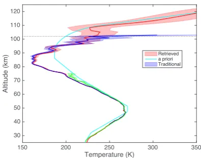
Figure 1: Two channel HSEQ temperature retrieval from Purple Crow Lidar measurements on 24 May
2012 (red curve) compared to the traditional method.
Rayleigh-scatter lidars are one of the best sources for temperature measurements in the middle atmosphere. Cooling in the middle at-mosphere associated with warming in the lower atmosphere is an important measurement in as-sessing atmospheric change, as, although it is still complex, interpreting the middle atmo-spheric temperatures is simpler than interpret-ing changes in surface temperature. However, the magnitude of the changes is small, on the order of ∼1◦ per decade. Thus, it is critical to have available an analysis technique that can perform a full uncertainty budget on a profile-by-profile basis. The OEM is a great choice for this application, and we applied it success-fully to the Western Purple Crow Lidar [1]. Figure 1 shows a 2-channel temperature re-trieval from Purple Crow Lidar measurements on 24 May 2012 (red curve). The figure also shows temperatures calculated using the tradi-tional method of Hauchecorne and Chanin for the low-gain (green) and high-gain (blue) data channels [2]. The a priori temperature profile used for the retrieval is the U.S. Standard Atmo-sphere (cyan curve). The horizontal dotted line is the height above which thea priori tempera-ture profile begins to make a significant contri-bution to the retrieval.
10- 10-4 10- 100
Uncertainty (K)
30 40 50 60 70 80 90 100 110 120
Altitude (km)
Stat p0 [O3] O3< Ray Exct ; Ray Exct <Ray <Ray(z) Gravity MMM Total
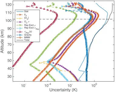
Figure 2: Uncertainty budget for the temperature retrieval in Figure 1. Details are given in the text.
profile for Rayleigh extinction (green squares), Rayleigh extinction cross section (blue dia-monds), variation of Rayleigh-scatter cross sec-tion with height (red triangles), gravity model (blue triangles), variation of mean molecular mass with height (orange triangles) and total uncertainty (black line). The horizontal dashed line is the height above which thea priori tem-perature profile makes a significant contribution to the retrieval.
Water Vapor (g/kg)
10- 10-1 100 101
Altitude (km)
0 2 4 6 8 10 12 14
Traditional OEM Sonde a priori
Figure 3: Four channel temperature retrieval of water vapour from the MeteoSwiss RALMO lidar on 5 September 2009 (red curve) compared to the
traditional method.
After success with temperature retrieval, we
ap-plied the OEM to the retrieval of water va-por using measurements from the MeteoSwiss RALMO lidar [3]. The RALMO water vapor measurements, in terms of data quality and calibration, are among the best available in the world. In addition, ancillary instruments such as radiosondes and microwave radiome-ters are available in Payerne for validation of the RALMO measurements. Figure 3 shows the retrieved water vapor mixing ratio (red curve) using the OEM on 5 September 2009. The blue curve is the mixing ratio using the traditional analysis method. The green curve is the ra-diosonde measurement. The sonde is launched at the start of the 30 min RALMO average. The dot-dashed line is thea priorimixing ratio pro-file used by the OEM. The horizontal dashed line shows the height below which the retrieval is due primarily to the measurement and not the a priori.
In this paper we will discuss two technical as-pects of applying OEM to lidar measurements, calculation of analytic forms for the Jacobians and practical considerations for working with non-linear counting systems.
Retrieval & Model Parameters
, )
cost= [y−F(ˆx,b)]TS−1
y [y−F(ˆx,b)] + [ˆx−xa]TS−a1[ˆx−xa]
minimize:
measurement = Forward Model + detector noise
a priori estimate & covariances
a, Sa, Sy)
Retrieved Parameters & Uncertainties The Optimal Estimation Method
Uncertainties: etrieved parameters,
model parameters, model smoothing
Rodgers, C. D. (2011), Inverse Methods for Atmospheric Sounding: Theory and Practice, World Scientific.
y=F(x,b) +✏
xa Sa, Sy
x, b
Figure 4: The OEM procedure. The retrieval is
computed from an a priori stateaof the retrieval
vectorx, model parameters,band covariancesS
using measurements,y.
2 FORWARD MODELS
10- 10-4 10- 100
Uncertainty (K)
30 40 50 60 70 80 90 100 110 120
Altitude (km)
Stat p0 [O3] O3< Ray Exct ; Ray Exct <Ray <Ray(z) Gravity MMM Total
Figure 2: Uncertainty budget for the temperature retrieval in Figure 1. Details are given in the text.
profile for Rayleigh extinction (green squares), Rayleigh extinction cross section (blue dia-monds), variation of Rayleigh-scatter cross sec-tion with height (red triangles), gravity model (blue triangles), variation of mean molecular mass with height (orange triangles) and total uncertainty (black line). The horizontal dashed line is the height above which thea priori tem-perature profile makes a significant contribution to the retrieval.
Water Vapor (g/kg)
10- 10-1 100 101
Altitude (km)
0 2 4 6 8 10 12 14
Traditional OEM Sonde a priori
Figure 3: Four channel temperature retrieval of water vapour from the MeteoSwiss RALMO lidar on 5 September 2009 (red curve) compared to the
traditional method.
After success with temperature retrieval, we
ap-plied the OEM to the retrieval of water va-por using measurements from the MeteoSwiss RALMO lidar [3]. The RALMO water vapor measurements, in terms of data quality and calibration, are among the best available in the world. In addition, ancillary instruments such as radiosondes and microwave radiome-ters are available in Payerne for validation of the RALMO measurements. Figure 3 shows the retrieved water vapor mixing ratio (red curve) using the OEM on 5 September 2009. The blue curve is the mixing ratio using the traditional analysis method. The green curve is the ra-diosonde measurement. The sonde is launched at the start of the 30 min RALMO average. The dot-dashed line is thea priorimixing ratio pro-file used by the OEM. The horizontal dashed line shows the height below which the retrieval is due primarily to the measurement and not the a priori.
In this paper we will discuss two technical as-pects of applying OEM to lidar measurements, calculation of analytic forms for the Jacobians and practical considerations for working with non-linear counting systems.
Retrieval & Model Parameters
, )
cost= [y−F(ˆx,b)]TS−1
y [y−F(ˆx,b)] + [ˆx−xa]TS−a1[ˆx−xa]
minimize:
measurement = Forward Model + detector noise
a priori estimate & covariances
a, Sa, Sy)
Retrieved Parameters & Uncertainties The Optimal Estimation Method
Uncertainties: etrieved parameters,
model parameters, model smoothing
Rodgers, C. D. (2011), Inverse Methods for Atmospheric Sounding: Theory and Practice, World Scientific.
y=F(x,b) +✏
xa Sa, Sy
x, b
Figure 4: The OEM procedure. The retrieval is
computed from an a priori stateaof the retrieval
vectorx, model parameters,band covariancesS
using measurements,y.
2 FORWARD MODELS
Figure 4 shows the basics of the Optimal Es-timation Method [3]. Our retrievals are “first-principle retrievals;” that is, our forward model
(FM) includes all the instrumental and atmo-spheric parameters necessary to reproduce the raw measurements.
Our forward models are based on the lidar equation. For Rayleigh-scatter temperature re-trievals we use the following form of the lidar equation for the true counts
Nt(z) =CT2
ψ(z)
z2 p(z)
kT(z)+Bt (1)
where in this compact form all the instrumen-tal parameters and constants are in the function
ψ, except for the lidar constantCwhich is ex-plicitly shown as it is often a retrieved quan-tity. The atmospheric transmission is T. The true background,Bt, can be constant or the an-alytical form of the background appropriate to a given system. The pressure,p(z)can be spec-ified or computed from the temperature using the assumption of hydrostatic equilibrium [1].
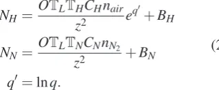
Water vapour mixing ratio retrievals require a more complex set of equations, as many wa-ter vapour lidars will have 4 channels (2 digital and 2 analog) for nitrogen (N) and water vapour (H). For the linear case, applicable to analog systems or low-gain photomultipliers, the true counts are given by:
NH=
OTLTHCHnair
z2 e
q′
+BH
NN=
OTLTNCNnN2
z2 +BN
q′=lnq.
(2)
Here the overlap function, O, varies with alti-tude,nis number density and the transmission reflects the inelastic scattering process. A log retrieval is used as water vapour mixing ratio, q, cannot be negative.
3 PRACTICAL JACOBIANS
The derivative of the FM,F, with respect to the retrieval vector,x is called the kernel,K. The
kernel is am×kmatrix whose elements are:
Ki j =
∂Fi(x)
∂xj
. (3)
Since K is a matrix of derivatives it can also be called the Jacobian (which is the term we will use, although in atmospheric science Kis sometimes called the weighting function).
The size of the Jacobian, that is, the number of retrieval parametersk, in relation to the number of independent measurements m, relates to the regularization of the problem. Whenm<kthe
problem is ill-posed (under-determined); when m>k the problem is over-constrained
(over-determined). Our lidar inversions have been re-stricted to the over-constrained situation.
To calculate the Jacobians, consider a retrieval of temperature from Rayleigh-scatter measure-ments for a system with 2 detection channels, which could be analog, digital or a combination of both and at different height resolutions. The data vector hasmdetector samples,y, defined at l1heights for the first channel andl2heights for the second channel, wherel1+l2=m. We want to retrievex(k)quantities consisting of, for ex-ample, temperature at some number of retrieval heights ≤k, dead time(s) and background(s) depending on the number of channels.
Themcolumns of the Jacobian contain the sen-sitivity of a measurement to the retrieval vector. Parameters are retrieved on the retrieval grid, using the measurement vector specified on the data grid.
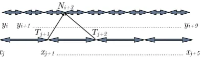
To visualize this consider a measurement vector comprised of a single channel of photocounts from which you want to retrieve temperature. The data grid is then a series of photocount measurements as a function of time (height) as shown in Figure 5.
xj xj+1 ……….……….…. xj+5
yi yi+1 ……… yi+9
Tj+1 Tj+2
Ni+3
Figure 5: Interpolation of a retrieved parameter (here temperature, T ) to photocounts, N, on the
data grid.
data grid to evaluate the lidar equation, the FM performs an interpolation of temperature from the retrieval grid to the data grid. We choose to use linear interpolation. Linear interpolation is a reasonable choice for these retrievals as the both the data and retrieval grid spacing is much less than an atmospheric scale height. Using the Chain Rule we write the temperature Jacobian as:
KTi j =
∂Fi(T)
∂Ti ·∂Ti
∂Tj
=∂Fi(T) ∂Ti
·
zj+1−zi
zj+1−zj
(4)
where the second term on the right hand side of Eq. (4) is due to the interpolation of the temper-ature on the retrieval grid to the data grid.
3.1 Analytical Derivatives
It is often not possible to calculate the analyti-cal derivative of a model or retrieval parameter in the FM, in which case a numerical deriva-tive can be calculated. Typically this derivaderiva-tive can be calculated using a simple finite differ-ence scheme. However, if the analytical deriva-tive can be determined, its exact form is a bet-ter choice than the numerical derivative. Some of the analytical derivatives are quite simple, such as for the lidar constant or a constant back-ground. Others are not possible, such as the temperature dependence of the Rayleigh-scatter FM under the assumption of hydrostatic
equi-librium, whereT additionally appears in the in-tegral used to determine pressure.
One Jacobian which can be determined analyt-ically is the derivative of the FM with respect to density. Consider the simpler case where optical depth (or transmission) is not being re-trieved, so transmission is specified on the data grid and an interpolation is not required. From Eq. (1) we see, using the Chain Rule, that the Jacobian of the FM with respect to density is:
∂Nt,ℓ
∂ni
=∂Nt,ℓ
∂Tℓ
×∂Tℓ
∂ni
(5)
whereℓandirange from 1 tomto form am×m
matrix. For discrete measurements the optical depth,τ, is given by
τℓ= ℓ
∑
i=1
σni∆z (6)
for equally spaced measurements and a con-stant cross section with altitude, σ, as in the case of water vapour and temperature retrievals. Note thatτ can be a specific optical depth, e.g. aerosol optical depth, as required. The trans-mission is then
Tℓ=exp
−
ℓ
∑
i=1
σni∆z
=
ℓ
∏
i=1
exp(−σni∆z),
(7)
where from the product above we see that the transmission Jacobian is:
∂Tℓ
∂ni
=−σTℓ∆zfori≤ℓ
=0 fori> ℓ.
(8)
We can now calculate the Jacobian with respect to density using Eqs. (5) and (8):
∂Nt,ℓ
∂ni
=−2(Nt,ℓ−Bt,ℓ)σ∆zfori≤ℓ
=0 fori> ℓ.
(9)
This form of the Jacobian is fast computation-ally and avoids any numerical issues with the exponential quantities involved.
3.2 Effect of Detector Saturation
The FMs given in Eqs. (1) and (2) refer to the
truecount rate. Systems which measure in the daytime or have large dynamic range may have signals which are significantly nonlinear due to limitations in the detection system. For in-stance, for daytime water vapour retrievals the background count rate is extremely large and the observed background counts are not equal to the true (corrected) counts. Furthermore, in the specification of the parameters for the re-trievals, the background term is estimated using the observed counts, not the true counts, so this difference must be accounted for in all quanti-ties in the FM. Consider a non-paralyzable sys-tem where the observed counts are related to the true counts by
No=
Nt
1+γNt
(10)
whereγ is the counting system dead time. The derivative of the observed counts with respect to the true counts is then
∂No
∂Nt
= (1−γNo)2. (11)
To apply our previous result for the Jacobian of the FM with respect to density for the non-linear case, we must find the derivative of the observed photocounts with respect ton, using the observed photocountsNo and the observed
background, Bo. Using the Chain Rule and
Eq. (9) we can show that
∂No,ℓ
∂ni
=∂No,ℓ
∂Nt,ℓ
·∂Nt,ℓ
∂ni
= (1−γNo,ℓ)
2·
−2
No,ℓ
1−γNo,ℓ
−Bo,ℓ
(σ∆z)
.
(12)
4 CONCLUSIONS
While each different type of scattering process requires a different FM, many of the retrieval and model parameters are the same. We demon-strated two tricks common to all retrievals, one an efficient analytical form for the transmission density Jacobian and the other inclusion of de-tector nonlinearity in the Jacobians. Currently, we are in the processes of developing general retrieval tools for use by the community in ap-plying the OEM, which incorporate these re-sults as well as some other finer points of the retrieval mechanics we have learned in devel-oping these techniques.
ACKNOWLEDGEMENTS
We thank C. Dennison for advice on the cal-culation of the transmission Jacobian. This project has been supported by the Natural Sciences and Engineering Research Council (NSERC Discovery Grant & CREATE), Cana-dian Space Agency (CSA) and MeteoSwiss.
References
[1] Sica, R. J., and A. Haefele, 2015: Re-trieval of temperature from a multiple-channel Rayleigh-scatter lidar using an optimal esti-mation method,Appl. Opt.54(8), 1872-1889.
[2] Hauchecorne, A., and M. Chanin, 1980: Den-sity and temperature profiles obtained by lidar between 35 and 70 km, Geophys. Res. Lett., 7(8), 565-568.
[3] Sica, R. J., and A. Haefele, 2016: Retrieval of water vapor mixing ratio from a multiple channel Raman-scatter lidar using an optimal estimation method, Appl. Opt. 55 (4), 763-777.