c
Owned by the authors, published by EDP Sciences, 2017
CMS trigger performance
Silvio Donato1,aon behalf of the CMS Collaboration
1University of Zurich
Abstract. During its second run of operation (Run 2), started in 2015, the LHC will deliver a peak instantaneous luminosity that may reach 2·1034cm−2s−1with an average
pileup of about 55, far larger than the design value. Under these conditions, the online event selection is a very challenging task. In CMS, it is realized by a two-level trigger system: the Level-1 (L1) Trigger, implemented in custom-designed electronics, and the High Level Trigger (HLT), a streamlined version of the offline reconstruction software
running on a computer farm.
In order to face this challenge, the L1 trigger has been through a major upgrade compared to Run 1, whereby all electronic boards of the system have been replaced, allowing more sophisticated algorithms to be run online. Its last stage, the global trigger, is now able to perform complex selections and to compute high-level quantities, like invariant masses. Likewise, the algorithms that run in the HLT have been greatly improved; in particu-lar, new approaches for the online track reconstruction lead to a drastic reduction of the computing time, and to much improved performances. This document will describe the performance of the upgraded trigger system in Run 2.
1 Introduction
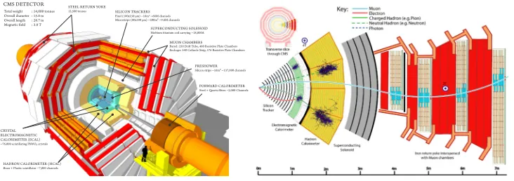
1.1 The CMS triggerThe Compact Muon Solenoid (CMS) is a multi-purpose experiment built at the Large Hadron Col-lider (LHC). It is made of a silicon tracker subdetector, a homogeneous electromagnetic calorime-ter, and a hadron calorimeter immersed in a magnetic field of 3.8 T produced by a superconducting solenoid. Muons are detected by gas-ionization subdetectors positioned in the flux-return yoke out-side the solenoid. Figure 1 shows the scheme of the CMS experiment and of the event reconstruction. More details about the CMS detector can be found in [1].
At the LHC, protons circulate in bunches with a time interval of 25 ns in two beams with opposite directions. As a consequence, proton bunches collide with a rate of 40 MHz, but only about 1 kHz of collisions is actually registered for data analysis. This limit is mainly determined by the offline
computing resources involved in the offline reconstruction. The events are selected online by a
two-level trigger system that reduces the rate from 40 MHz to 1 kHz.
The Level-1 trigger (L1) is made of customizable hardware and reduces the rate from 40 MHz to 100 kHz. The L1 trigger decision is taken in less than 4µs using a simplified readout of the calorimeter and muon subdetectors. As soon as an event is accepted by the L1 trigger, the full readout of the CMS
SUPERCONDUCTING SOLENOID Niobium titanium coil carrying ~18,000A
PRESHOWER Silicon strips ~16m2 ~137,000 channels SILICON TRACKERS
Pixel (100x150 μm) ~16m2 ~66M channels Microstrips (80x180 μm) ~200m2 ~9.6M channels
MUON CHAMBERS Barrel: 250 Drift Tube, 480 Resistive Plate Chambers Endcaps: 540 Cathode Strip, 576 Resistive Plate Chambers
FORWARD CALORIMETER Steel + Quartz fibres ~2,000 Channels STEEL RETURN YOKE
12,500 tonnes
HADRON CALORIMETER (HCAL) Brass + Plastic scintillator ~7,000 channels CRYSTAL ELECTROMAGNETIC CALORIMETER (ECAL) ~76,000 scintillating PbWO4 crystals
Total weight Overall diameter Overall length Magnetic field
: 14,000 tonnes : 15.0 m : 28.7 m : 3.8 T CMS DETECTOR
Figure 1.The subdetectors of the CMS experiment (left) and a schematic view of the different particles’ signature
inside the detector (right).
detector takes place. The maximum L1 trigger output rate (100 kHz) is defined by the readout of the detector.
The High Level Trigger (HLT) is a computing farm made of 26 thousands of cores that selects
events using software algorithms from a rate of 100 kHz down to∼ 1 kHz. The limit on the
aver-age computing time is 260 ms. Differently from L1 trigger, the HLT has access to the full detector
information.
2 The L1 trigger
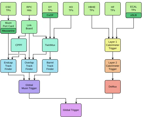
The L1 trigger has been entirely upgraded between 2013 and 2015, as part of the CMS Phase-1 up-grade [2]. Figure 2 shows a working scheme of the new L1 trigger. The L1 trigger event reconstruction starts from a simplified readout performed in the calorimeter (HCAL, ECAL, HF) and in the muons chambers (CSC, DT, RPC), called trigger primitives. No tracker information is accessible to the L1 trigger. Trigger primitives are then combined to form calorimetric towers and to link compatible muon
hits together. Afterwards, they are used to form the L1 trigger objects: muons, electrons/photons,τ,
jets, missing transverse energy and total transverse energy. Eventually, the event is accepted if the L1 trigger objects fulfill at least one of the conditions defined by the L1 menu, eg. one muon with
pT >15 GeV and missing transverse energy larger than 100 GeV.
The next paragraphs will show the performance in the reconstruction of the L1 trigger objects.
2.1 The L1 electron/photon
In the L1 trigger system photons and electrons cannot be distinguished. Many improvements have
been achieved with the Phase-I upgrade in the electron/photon reconstruction, and some of them have
been fully exploited recently in 2017. The left plot in Fig. 3 compares the efficiency curves obtained
in 2016 and 2017 for two single electron/photon triggers having the same rate: in 2017 we lowered
the energy threshold by 2 GeV and improved the energy resolution of the L1 objects.
Furthermore, in 2017 a loose version of the electron/photon isolation has been introduced to be
mainly applied to the multi-object triggers in order to increase their efficiency. Figure 3 (right plot)
SUPERCONDUCTING SOLENOID Niobium titanium coil carrying ~18,000A
PRESHOWER Silicon strips ~16m2 ~137,000 channels SILICON TRACKERS
Pixel (100x150 μm) ~16m2 ~66M channels Microstrips (80x180 μm) ~200m2 ~9.6M channels
MUON CHAMBERS Barrel: 250 Drift Tube, 480 Resistive Plate Chambers Endcaps: 540 Cathode Strip, 576 Resistive Plate Chambers
FORWARD CALORIMETER Steel + Quartz fibres ~2,000 Channels STEEL RETURN YOKE
12,500 tonnes
HADRON CALORIMETER (HCAL) Brass + Plastic scintillator ~7,000 channels CRYSTAL ELECTROMAGNETIC CALORIMETER (ECAL) ~76,000 scintillating PbWO4 crystals
Total weight Overall diameter Overall length Magnetic field
: 14,000 tonnes : 15.0 m : 28.7 m : 3.8 T CMS DETECTOR
Figure 1.The subdetectors of the CMS experiment (left) and a schematic view of the different particles’ signature
inside the detector (right).
detector takes place. The maximum L1 trigger output rate (100 kHz) is defined by the readout of the detector.
The High Level Trigger (HLT) is a computing farm made of 26 thousands of cores that selects
events using software algorithms from a rate of 100 kHz down to∼ 1 kHz. The limit on the
aver-age computing time is 260 ms. Differently from L1 trigger, the HLT has access to the full detector
information.
2 The L1 trigger
The L1 trigger has been entirely upgraded between 2013 and 2015, as part of the CMS Phase-1 up-grade [2]. Figure 2 shows a working scheme of the new L1 trigger. The L1 trigger event reconstruction starts from a simplified readout performed in the calorimeter (HCAL, ECAL, HF) and in the muons chambers (CSC, DT, RPC), called trigger primitives. No tracker information is accessible to the L1 trigger. Trigger primitives are then combined to form calorimetric towers and to link compatible muon
hits together. Afterwards, they are used to form the L1 trigger objects: muons, electrons/photons,τ,
jets, missing transverse energy and total transverse energy. Eventually, the event is accepted if the L1 trigger objects fulfill at least one of the conditions defined by the L1 menu, eg. one muon with
pT >15 GeV and missing transverse energy larger than 100 GeV.
The next paragraphs will show the performance in the reconstruction of the L1 trigger objects.
2.1 The L1 electron/photon
In the L1 trigger system photons and electrons cannot be distinguished. Many improvements have
been achieved with the Phase-I upgrade in the electron/photon reconstruction, and some of them have
been fully exploited recently in 2017. The left plot in Fig. 3 compares the efficiency curves obtained
in 2016 and 2017 for two single electron/photon triggers having the same rate: in 2017 we lowered
the energy threshold by 2 GeV and improved the energy resolution of the L1 objects.
Furthermore, in 2017 a loose version of the electron/photon isolation has been introduced to be
mainly applied to the multi-object triggers in order to increase their efficiency. Figure 3 (right plot)
shows the efficiency of the single electron/photon trigger with standard and loose isolation.
Figure 2.Working scheme of the Phase-1 L1 trigger system. [2]
[GeV]
T
E
10 20 30 40 50 60 70 80 90 100
Efficiency
0 0.2 0.4 0.6 0.8 1
2017 Data, X=40 in GeV unit
2016 Data, X=42 in GeV unit
<PU> = 24
L1EG(X) OR L1EGIso(X-2) OR L1EGIsoEr(X-4) (2017) (13 TeV) -1
(2016) + 53 pb -1 221 pb
CMSPreliminary
[GeV]
T
E
10 20 30 40 50 60 70 80 90 100
Efficiency
0 0.2 0.4 0.6 0.8 1
SingleEG Isolation
Loose Isolation
(2017) (13 TeV) -1
53 pb
CMSPreliminary
L1 Single EG
Threshold: 38 GeV + Isolation
Figure 3. On the left, L1 trigger efficiency curve for an electron/photon object as a function of the offline
reconstructed supercluster transverse energy ET with the 2017 algorithm (blue) and the 2016 algorithm (red)
measured using tag-and-probe method on data. A geometrical matching between the electron supercluster and the L1 candidate is applied. The efficiency is drawn for the combination of the following triggers: e/γwith pT > XGeV without isolation requirements (EG) OR e/γwith pT > (X−2) GeV and isolation requirement
(EGIso) OR e/γwith pT >(X−4) GeV, isolation requirement and pseudorapidity|η|<2.1 (EGIsoEr). The two
curves are drawn for the thresholds X ensuring the same trigger rate. On the right, L1 trigger efficiency curve for
an electron/photon object as a function of the offline reconstructed supercluster transverse energy ET with 2017
tight EG isolation requirements and a pTthreshold of 25 GeV (blue) and emulated events with loose EG isolation
requirements and pT threshold of 25 GeV (red). The loose isolation allows to increase the efficiency for cross
[GeV]
, offline τ T
p
10 20 30 40 50 60 70 80 90 100
Efficiency
0 0.2 0.4 0.6 0.8 1
> 26 GeV
, L1
τ
T
Inclusive, E > 30 GeV
, L1
τ
T
Inclusive, E > 34 GeV
, L1
τ
T
Inclusive, E > 26 GeV
, L1
τ
T
Inclusive, E > 30 GeV
, L1
τ
T
Inclusive, E > 34 GeV
, L1
τ
T
Inclusive, E > 26 GeV
, L1
τ
T
Inclusive, E > 30 GeV
, L1
τ
T
Inclusive, E > 34 GeV
, L1
τ
T
Inclusive, E τ
L1T
CMS
2016 preliminary
(13 TeV)
-1
35.9 fb
[GeV]
, offline τ T
p
20 40 60 80 100 120 140
Efficiency
0 0.2 0.4 0.6 0.8 1
)
-1
Isolated, May-September (27.3 fb )
-1
Isolated, September-October (8.6 fb )
-1
Isolated, May-September (27.3 fb )
-1
Isolated, September-October (8.6 fb τ
L1T
CMS
2016 preliminary
(13 TeV)
-1
35.9 fb
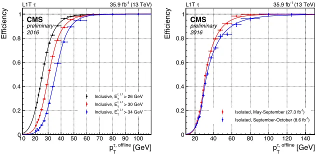
Figure 4.On the left, L1 trigger efficiency of inclusiveτ-seeds (i.e. without any requirement on the isolation at L1) as a function of the offlineτtransverse momentum. On the right, L1 trigger efficiency of isolatedτ-seeds (i.e. requiring the L1τcandidate to pass a cut on its isolation transverse energy) as a function of the offlineτ transverse momentum, for a L1ETthreshold of 30 GeV. The isolation criterion was tightened in September 2016 to cope with the increasing LHC luminosity. In the period May-September, the peak instantaneous luminosity was lower than 1.34×1034cm−2·s−1, while it has reached 1.53×1034cm−2·s−1in the September-October period.
[4]
2.2 The L1τ
The identification of hadronically-decayingτhas been significantly improved with the Phase-I up-grade. The higher granularity of the calorimeters allowed to tagτin a more sophisticated way, requir-ing isolation too. L1τenergy is calibrated as a function of the energy and pileup. The isolation cut depends on theτenergy,ηand pileup, in order to get a flatτefficiency. Figure 4 shows the efficiency
curve of the single object trigger, for different working points, for the isolated (left) and inclusive
(right) trigger. The resolution of L1τpT is about 20−25% at 30−50 GeV.
2.3 The L1 vector boson fusion
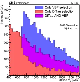
Another important achievement obtained with the Phase-I upgrade is a more powerful L1 trigger able to compute the invariant mass between objects. It has been exploited in a trigger dedicated to the search for theH→ττproduced through the vector boson fusion. The new trigger requires the pres-ence of twoτjets plus two forward/backward jets with a large invariant mass between them. Figure 5
shows the large acceptance gained by this new trigger as a function of the offline forward/backward jet
invariant mass, for a sample of simulatedH→ττevents produced through the vector boson fusion.
2.4 The L1 jet/MET
[GeV]
, offline τ T
p
10 20 30 40 50 60 70 80 90 100
Efficiency 0 0.2 0.4 0.6 0.8 1
> 26 GeV
, L1
τ
T
Inclusive, E > 30 GeV
, L1
τ
T
Inclusive, E > 34 GeV
, L1
τ
T
Inclusive, E > 26 GeV
, L1
τ
T
Inclusive, E > 30 GeV
, L1
τ
T
Inclusive, E > 34 GeV
, L1
τ
T
Inclusive, E > 26 GeV
, L1
τ
T
Inclusive, E > 30 GeV
, L1
τ
T
Inclusive, E > 34 GeV
, L1 τ T Inclusive, E τ L1T CMS 2016 preliminary (13 TeV) -1 35.9 fb [GeV] , offline τ T p
20 40 60 80 100 120 140
Efficiency 0 0.2 0.4 0.6 0.8 1 ) -1
Isolated, May-September (27.3 fb )
-1
Isolated, September-October (8.6 fb )
-1
Isolated, May-September (27.3 fb )
-1
Isolated, September-October (8.6 fb τ L1T CMS 2016 preliminary (13 TeV) -1 35.9 fb
Figure 4.On the left, L1 trigger efficiency of inclusiveτ-seeds (i.e. without any requirement on the isolation at L1) as a function of the offlineτtransverse momentum. On the right, L1 trigger efficiency of isolatedτ-seeds (i.e. requiring the L1τcandidate to pass a cut on its isolation transverse energy) as a function of the offlineτ transverse momentum, for a L1ETthreshold of 30 GeV. The isolation criterion was tightened in September 2016 to cope with the increasing LHC luminosity. In the period May-September, the peak instantaneous luminosity was lower than 1.34×1034cm−2·s−1, while it has reached 1.53×1034cm−2·s−1in the September-October period.
[4]
2.2 The L1τ
The identification of hadronically-decayingτhas been significantly improved with the Phase-I up-grade. The higher granularity of the calorimeters allowed to tagτin a more sophisticated way, requir-ing isolation too. L1τenergy is calibrated as a function of the energy and pileup. The isolation cut depends on theτenergy,ηand pileup, in order to get a flatτefficiency. Figure 4 shows the efficiency
curve of the single object trigger, for different working points, for the isolated (left) and inclusive
(right) trigger. The resolution of L1τpT is about 20−25% at 30−50 GeV.
2.3 The L1 vector boson fusion
Another important achievement obtained with the Phase-I upgrade is a more powerful L1 trigger able to compute the invariant mass between objects. It has been exploited in a trigger dedicated to the search for theH→ττproduced through the vector boson fusion. The new trigger requires the pres-ence of twoτjets plus two forward/backward jets with a large invariant mass between them. Figure 5
shows the large acceptance gained by this new trigger as a function of the offline forward/backward jet
invariant mass, for a sample of simulatedH→ττevents produced through the vector boson fusion.
2.4 The L1 jet/MET
At L1 trigger level, jets are reconstructed using only the calorimeters. Their reconstruction has been significantly improved with the Phase-I upgrade, especially thanks to the higher granularity of the calorimetric trigger primitives and a more advanced pileup correction. Similar improvements have been obtained for the missing and total transverse energy. Figure 6 shows the trigger efficiency curves
[GeV] jj offline m 400 600 800 1000 1200 1400 1600 1800 2000
Events/40 GeV 0 50 100 150 200 250 300 350 400 Preliminary
CMS (13 TeV)
2016 Simulation
τ τ →
VBF H Only VBF selection Only DiTau selection DiTau AND VBF
Figure 5.Gain from the L1 VBF seed (with at least one jet withET>110 GeV and at least two jets withET >35 GeV andmj j >620 GeV) with respect to the baseline Double Tau seed (at least 2 isolated taus withET >32 GeV and|η|<2.1) as a function of the offlinemj j. The offline selections are chosen to be tighter than online.
The events in each of the categories “Only VBF selection” and “Only Di-Tau selection” are events that fired only one of the triggers and pass only the offline selection corresponding to that trigger. The events in the category
“Di-Tau AND VBF” fire both triggers and pass both offline selections. [4]
(GeV) T Offline Jet E
100 200 300 400 500
Efficiency 0 0.2 0.4 0.6 0.8 1
> 36 GeV
T
L1 Jet E > 68 GeV
T
L1 Jet E > 128 GeV
T
L1 Jet E > 200 GeV
T
L1 Jet E
CMS Preliminary 2017 Data 8.8 fb-1 (13 TeV)
| < 3.0
η
|
Offline MET (GeV)
0 50 100 150 200 250 300 350 400
Efficiency 0 0.2 0.4 0.6 0.8 1
CMS Preliminary 2017 Data 8.8 fb-1 (13 TeV)
L1 MET > 40 GeV L1 MET > 80 GeV L1 MET > 100 GeV L1 MET > 120 GeV
| < 5.0 η |
Figure 6. On the left, efficiency curves for the L1 single jet triggers using events with an offline muon as a
function of offline jet transverse energy reconstructed with the anti-kt (R=0.4) algorithm and|η|<3. Offline and
L1 jets are matched with∆R<0.4. On the right, efficiency curves for the L1 missing energy trigger using events
with an offline muon as a function of offline missing transverse energy. [5]
as a function of the offline jet transverse energyET for severalET thresholds of the single jet trig-ger (on the left), and as a function of the offline missing transverse energy (MET) for several MET
thresholds triggers (on the right).
2.5 The L1 muon
η
2.5
− −2−1.5 −1−0.5 0 0.5 1 1.5 2 2.5
L1 muon efficiency
0 0.2 0.4 0.6 0.8 1
Tight L1 quality 25 GeV ≥ T L1 p
> 30 GeV T Offline p
CMSpreliminary 2017 data 8.5 fb-1 (13 TeV)
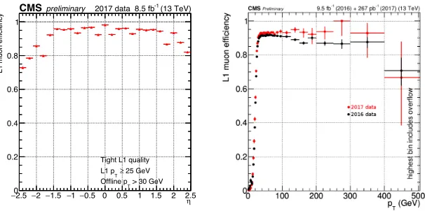
Figure 7. Trigger efficiency for the single muon L1 trigger with pT > 25 GeV. On the left, efficiency as a
function of the offline reconstructed muonηwithpT >30 GeV [3]. On the right, efficiency as a function of the
offline reconstructed muonpT[6]. A more recent version of the plots is available at [7].
The muon reconstruction has been improved by a more sophisticated track finder that allowed to increase the efficiency. Figure 7 shows the L1 single muon efficiency as a function ofη(left) and pT (right). The latter plot shows also a further improvement that has been obtained in 2017 for highpT muons.
3 The HLT trigger
3.1 The HLT pathThe output rate of the L1 trigger is about 100 kHz. The HLT trigger reduces this rate further down
∼1 kHz running software algorithms. The limit on the average computing time is fixed by the number of cores and the input rate:∼26000 cores/100 kHz=∼260 ms.
The HLT is composed of hundreds of HLT paths, that are sequences of reconstructing and filtering modules. As soon as an event is rejected by a filter, the subsequent modules are not run. The idea is to reconstruct firstly quick objects, cut on them, and then reconstruct more precise/slow objects, to keep
a low average computing time.
In order to explain in some details the functioning of an HLT trigger path, we consider as an example a hypothetical trigger that requires MET>120 GeV plus onebtagged jet [8].
A typical sequence of selections used in a HLT path withbtagging uses the following information: L1 seed, calorimetric objects,btagging with regional tracking, and PF objects (the numbers shown are purely indicative since they depend on many variables like pileup, CPU and so forth).
• L1 seed[Input rate∼100 kHz; Time<1 ms]. Each HLT path runs over every event accepted by the L1 trigger (∼100 kHz). The first cut of a HLT path is the selection of a specific L1 trigger seed, i.e. a specific trigger in the L1 menu or a logical combination of them. In the example, the L1 seed used is MET>70 GeV. The cut on the L1 seed reduces the rate by a factor∼10.
η
2.5
− −2−1.5 −1−0.5 0 0.5 1 1.5 2 2.5
L1 muon efficiency
0 0.2 0.4 0.6 0.8 1
Tight L1 quality 25 GeV ≥ T L1 p
> 30 GeV T Offline p
CMSpreliminary 2017 data 8.5 fb-1 (13 TeV)
Figure 7. Trigger efficiency for the single muon L1 trigger with pT > 25 GeV. On the left, efficiency as a
function of the offline reconstructed muonηwithpT >30 GeV [3]. On the right, efficiency as a function of the
offline reconstructed muonpT[6]. A more recent version of the plots is available at [7].
The muon reconstruction has been improved by a more sophisticated track finder that allowed to increase the efficiency. Figure 7 shows the L1 single muon efficiency as a function ofη(left) andpT (right). The latter plot shows also a further improvement that has been obtained in 2017 for highpT muons.
3 The HLT trigger
3.1 The HLT pathThe output rate of the L1 trigger is about 100 kHz. The HLT trigger reduces this rate further down
∼1 kHz running software algorithms. The limit on the average computing time is fixed by the number of cores and the input rate:∼26000 cores/100 kHz=∼260 ms.
The HLT is composed of hundreds of HLT paths, that are sequences of reconstructing and filtering modules. As soon as an event is rejected by a filter, the subsequent modules are not run. The idea is to reconstruct firstly quick objects, cut on them, and then reconstruct more precise/slow objects, to keep
a low average computing time.
In order to explain in some details the functioning of an HLT trigger path, we consider as an example a hypothetical trigger that requires MET>120 GeV plus onebtagged jet [8].
A typical sequence of selections used in a HLT path withbtagging uses the following information: L1 seed, calorimetric objects,btagging with regional tracking, and PF objects (the numbers shown are purely indicative since they depend on many variables like pileup, CPU and so forth).
• L1 seed[Input rate∼100 kHz; Time<1 ms]. Each HLT path runs over every event accepted by the L1 trigger (∼100 kHz). The first cut of a HLT path is the selection of a specific L1 trigger seed, i.e. a specific trigger in the L1 menu or a logical combination of them. In the example, the L1 seed used is MET>70 GeV. The cut on the L1 seed reduces the rate by a factor∼10.
• L2 - Calorimetric selection[Input rate∼10 kHz; Time∼50 ms].Since the reconstruction of the calorimetric objects (e.g. calorimetric MET) is very fast, it takes place usually just after the L1 seed selection. The resolution of these objects is worse compared to the PF objects, but they can
be reconstructed in only∼50 ms, 20 times faster than the corresponding PF objects. Calorimetric objects can be reconstructed for any event accepted by the L1 trigger. When the selection criteria are applied to calorimetric objects tracks are not available, and hence, for instance, we cannot tag pileup jets. In the example, the L2 cuts used are: calorimetric MET>70 GeV and two calorimetric jets withpT >30 GeV and|η|<2.6. Usually, the L2 cuts reduce the rate by a factor 5–10.
• L3 - Regional tracking[Input rate∼2 kHz; Time∼100 ms]. As tracking is a slow process, the tracker information is not used in the L1 and L2 stages. Still, tracks are essential for many tasks like distinguishing between photons and electrons, identifybandτjets, evaluate the track-based lepton isolation, and measure precisely the lepton momentum. To take advantage of the tracking information at HLT, two strategies are used: run tracking over a small fraction of events and only in the regions of interest (cones with∆R=0.4 around the calorimetric objects). In the example, the regional tracking is used to performbtagging and it is used to reduce the rate down to∼500 Hz.
• PF sequence[Input rate∼500 Hz; Time∼1000 ms].The Particle Flow (PF) sequence is the most accurate and slow reconstruction sequence available at HLT. Usually, the tightest cuts at HLT are applied to PF objects. The PF sequence used at HLT is similar to the offline version, but it uses
a simplified version of tracking. The HLT PF tracking reconstructs only tracks close to leading primary vertices and with pT > 500 MeV. Then, tracks are linked to objects reconstructed with the calorimeters and the muon chambers. The PF sequence reconstructs any high level objects: jets, MET, electrons, photons, muons, taus, etc. In some HLT paths, the PF tracks are also used to performbtagging on PF jets. In the example, the PF objects are used for the final cut MET > 120 GeV bringing the rate down to∼10 Hz.
The input rate, time, and average-per-event time of each HLT step is reported in Table 1. Note that even if the PF sequence needs∼1000 ms, it increases the average path time by only∼5 ms because it is run at∼500 Hz.
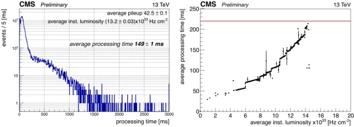
Figure 8 shows the computing time distribution of the HLT in a run of 2016, when an instantaneous luminosity of 1.5·1034Hz cm−2 was delivered by the LHC. In 2016, the number of cores was 22 k, and it has been increased in 2017 to 26 k. Moreover, the HLT reconstruction has been improved and the global timing decreased.
Table 1.Time and rate of the object reconstruction of an hypothetical MET+btagging trigger. The numbers
are purely indicative since they depend on many variables. The numbers reported are the running time, the input rate, and the average time spent per event. The last column can be calculated as the running time multiplied by
the input rate and divided by the global HLT input rate (∼100 kHz). For reference, the limit at HLT on the average global latency is∼260 ms and on the rate is∼1 kHz.
Object reconstruction ∼Time ( ms) ∼Rate ( Hz) ∼Av. time ( ms)
L1 variables <1 105 <1
Jet/MET 50 104 5
Regional tracking (btagging) 100 2000 2
Particle flow 1000 500 5
Figure 8. On the left, HLT computing time in a run with average instantaneous luminosity equal to 1.3·1034cm−2s−1 and pileup of 42.5. The processing time was measured on an "Ivy Bridge" Intel Xeon
E5-2650v2 processor, running one single job. On the right, average HLT computing timing vs instantaneous lumi-nosity. Both plots have been obtained with 2016 data. [9]
3.2 The HLT rate
The average HLT rate limit over the year is about 1 kHz. This limitation comes from the computing resources involved in the offline reconstruction, while the data acquisition system is able to transfer
up to 5−6 kHz and the space on tape would allow us to record up to 2 kHz. Since this limit applies to the average HLT rate, we can have short periods with peak rate above 1 kHz.
We can overcome the 1 kHz limit in two ways. For several exotic searches, we store only online objects with a rate of∼5 kHz (“data scouting”) that will be used directly in data analyses, skipping the offline reconstruction. We can also save more data on tape without running any offline reconstruction
(“parking”). During Run-2, about 10% of scouting data (rate∼500 Hz) has been “parked” saving the full event content. The rationale is to allow in the future to confirm/reject a possible hint of New
Physics found by data scouting analyses. Furthermore, we record temporary additional data with no offline reconstruction for trigger commissioning, e.g. for trigger rate estimate.
3.3 The HLT tracking
In 2017, the pixel subdetector has been upgraded. The new subdetector has one more layer, both in the barrel and in the endcap, and can work efficiently even at high luminosity. The HLT tracking has
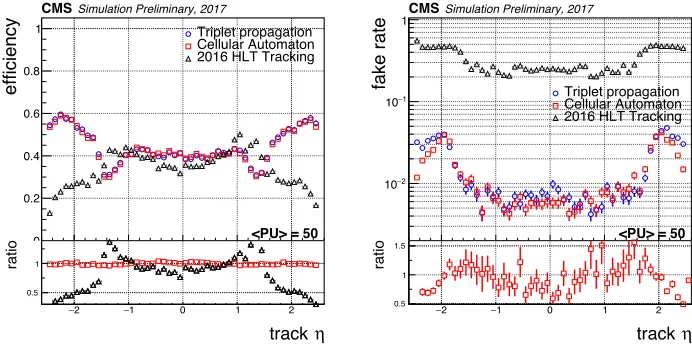
been updated to exploit the four layers, especially in the track seeding. Figure 9 shows the online track seeding efficiency, on the left side, and fake rate, on the right side, as a function ofη. The efficiencies
and fake-track rates have been evaluated for the old pixel subdetector (“2016 HLT tracking”), for the new pixel subdetector with the old pixel track seeding based on triplets (“Triplet propagation”), and for the new pixel subdetector with the new track seeding based on quadruplets (“Cellular Automaton”). The plots show that with the new pixel subdetector we have a fake rate decrease by more than a factor ten and an efficiency increase, especially in the endcaps. The new track seeding shows a similar
efficiency and a lower fake rate. The main difference between the two algorithms is in computing time.
Table 2 shows the computing time expected for the different tracking algorithms: the new version is
Figure 8. On the left, HLT computing time in a run with average instantaneous luminosity equal to 1.3·1034cm−2s−1and pileup of 42.5. The processing time was measured on an "Ivy Bridge" Intel Xeon
E5-2650v2 processor, running one single job. On the right, average HLT computing timing vs instantaneous lumi-nosity. Both plots have been obtained with 2016 data. [9]
3.2 The HLT rate
The average HLT rate limit over the year is about 1 kHz. This limitation comes from the computing resources involved in the offline reconstruction, while the data acquisition system is able to transfer
up to 5−6 kHz and the space on tape would allow us to record up to 2 kHz. Since this limit applies to the average HLT rate, we can have short periods with peak rate above 1 kHz.
We can overcome the 1 kHz limit in two ways. For several exotic searches, we store only online objects with a rate of∼5 kHz (“data scouting”) that will be used directly in data analyses, skipping the offline reconstruction. We can also save more data on tape without running any offline reconstruction
(“parking”). During Run-2, about 10% of scouting data (rate∼500 Hz) has been “parked” saving the full event content. The rationale is to allow in the future to confirm/reject a possible hint of New
Physics found by data scouting analyses. Furthermore, we record temporary additional data with no offline reconstruction for trigger commissioning, e.g. for trigger rate estimate.
3.3 The HLT tracking
In 2017, the pixel subdetector has been upgraded. The new subdetector has one more layer, both in the barrel and in the endcap, and can work efficiently even at high luminosity. The HLT tracking has
been updated to exploit the four layers, especially in the track seeding. Figure 9 shows the online track seeding efficiency, on the left side, and fake rate, on the right side, as a function ofη. The efficiencies
and fake-track rates have been evaluated for the old pixel subdetector (“2016 HLT tracking”), for the new pixel subdetector with the old pixel track seeding based on triplets (“Triplet propagation”), and for the new pixel subdetector with the new track seeding based on quadruplets (“Cellular Automaton”). The plots show that with the new pixel subdetector we have a fake rate decrease by more than a factor ten and an efficiency increase, especially in the endcaps. The new track seeding shows a similar
efficiency and a lower fake rate. The main difference between the two algorithms is in computing time.
Table 2 shows the computing time expected for the different tracking algorithms: the new version is
five time faster than the old tracking with the new pixel subdetector. Moreover, the new algorithm is ready to be ported to GPU. This would further decrease timing by a factor ten, as shown in the last row of the table.
η
track 2
− −1 0 1 2
efficiency
0 0.2 0.4 0.6 0.8
1 Triplet propagation
Cellular Automaton 2016 HLT Tracking Simulation Preliminary, 2017
CMS
<PU> = 50
η
track
2
− −1 0 1 2
ratio
0.5
1 trackη
2
− −1 0 1 2
fake rate
2 −
10
1 −
10 1
Triplet propagation Cellular Automaton 2016 HLT Tracking Simulation Preliminary, 2017
CMS
<PU> = 50
η
track
2
− −1 0 1 2
ratio
0.5 1 1.5
Figure 9.HLT Pixel Tracking efficiency (left) and fake-rate (right) as a function ofηfor 1000t¯tsimulated events with superimposed pileup collisions of 50, for three different algorithms. The Cellular Automaton and the Triplet
Propagation algorithms with Phase-I pixel subdetector are compared to the pixel tracking running at HLT during 2016 with the Phase-0 pixel subdetector. The ratio between the 2016 HLT Pixel Tracking and Triplet Propagation with respect to the Cellular Automaton plot is also shown. The inefficiency in the interval 1.0<|η|<1.5 is due to the non hermetic four-hits coverage transitioning from the barrel to the forward region. The asymmetry of the distribution in eta is due to the realistic position of the beamspot, slightly displaced with respect to the origin. [10]
3.4 The HLT jet and MET/HT
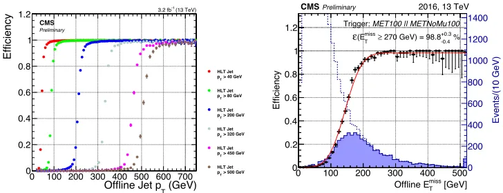
At HLT, tracking is used to run a simplified version of the Particle Flow (PF) algorithm to improve the objects reconstruction, especially on jets and MET. As a reference, thepT relative resolution of a simulated jet withpT ∼30 GeV is of 28% for the online calorimetric jets and of 18% for online PF jets. Figure 10 shows the efficiency as a function of the offline reconstructed quantity for single jet
triggers with differentpT thresholds, on the left side, and for missing transverse energy triggers with different MET thresholds, on the right side.
Table 2.Timing performance of different quadruplets generators at HLT PixelTracks for 1000 eventst¯t
simulated for the Phase-I subdetector with superimposed pileup collisions of 50. Tracking was executed on every event. The CPU used for tests is a Intel Core i7-4771 CPU 3.50 GHz, 4 cores, 8 simultaneous multi-threading threads. The GPU used is a NVIDIA GTX 1080. In all the cases the CMSSW framework was
configured to use 8 threads.
Quadruplet Algorithm Time per event speedup wrt. 2016 2016 Pixel Tracks (29.3±13.1) ms 1×
CPU Cellular Automaton (14.0±6.2) ms 2.1×
Triplet Propagation (72.1±25.7) ms 0.4×
100 200 300 400 500 600 700 0
100 200 300 400 500 600 700 800 900
(GeV)
T
Offline Jet p 0 100 200 300 400 500 600 700
Efficiency
0 0.2 0.4 0.6 0.8 1
1.2 3.2 fb-1 (13 TeV)
CMS
Preliminary
> 40 GeV
T
p HLT Jet
> 80 GeV
T
p HLT Jet
> 200 GeV
T
p HLT Jet
> 320 GeV
T
p HLT Jet
> 450 GeV
T
p HLT Jet
> 500 GeV
T
p HLT Jet
[GeV]
miss T
Offline E 0 100 200 300 400 500
Efficiency
0 0.2 0.4 0.6 0.8 1 1.2
Events/(10 GeV)
0 200 400 600 800 1000 1200 1400
MET100 || METNoMu100
Trigger:
%
-0.4 +0.3
270 GeV) = 98.8
≥
miss T
(E
ε Preliminary
CMS 2016, 13 TeV
Figure 10. On the left, trigger efficiency for jets at High Level trigger (HLT) as a function of the offline jet
transverse momentum. The events are triggered by a single muon. The jets are restricted to a pseudorapidity range|eta|<3.0. In each efficiency curve, the numerator is the number of offline jets which are matched to the
online jets inside a dR<0.2 and of which the transverse momentum is larger than trigger threshold. The
denom-inator is the number of offline jets. On the right, efficiency of the logical OR of the HLT PFMET[NoMu]100
PFMHT[NoMu]100 IDTight triggers as a function of offline missing transverse energy measured in 13 TeV data
selected with online requirements of a 25 GeV electron. [11][12]
3.5 The HLTbtagging
At HLT, onlinebtagging is performed in two different ways. In the first one,btagging is evaluated
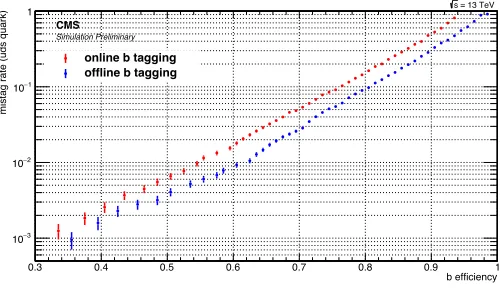
using tracks reconstructed in the PF sequence. It is used tobtag PF jets. The second one is used tob tag calorimetric jets before running the PF sequence. It exploits a dedicated regional tracking around the leading calorimetric jets using a primary vertex constraint, allowing to reduce the computing timing from 356.7 ms (PF tracking) to 86.9 ms. More details are available in [8]. Figure 11 shows the btagging efficiency vs light-jet fake-rate for the offline and onlinebtagging of calorimetric jets.
3.6 The HLT electron
Electrons are reconstructed at HLT using a dedicated tracking algorithm - the Gaussian-sum filter - that was developed for particles with a strong bremsstrahlung energy loss. The track information is then combined with the energy deposited in the electromagnetic calorimeters. The online electron reconstruction efficiency is very high (>99%). Tight isolation/identification cuts are applied to reduce
rate originated from jets and photon conversions, allowing to reduce the trigger threshold inpT. After tight cuts, the online electron efficiency is of∼ 90% in barrel and∼ 80% in endcaps, as shown in
Figure 12. The efficiency has been measured using a tag-and-probe method onZ→eeevents.
3.7 The HLTτ
100 200 300 400 500 600 700 0 100 200 300 400 500 600 700 800 900 (GeV) T
Offline Jet p 0 100 200 300 400 500 600 700
Efficiency 0 0.2 0.4 0.6 0.8 1
1.2 3.2 fb-1 (13 TeV)
CMS
Preliminary
> 40 GeV
T
p HLT Jet
> 80 GeV
T
p HLT Jet
> 200 GeV
T
p HLT Jet
> 320 GeV
T
p HLT Jet
> 450 GeV
T
p HLT Jet
> 500 GeV
T p HLT Jet [GeV] miss T Offline E 0 100 200 300 400 500
Efficiency 0 0.2 0.4 0.6 0.8 1 1.2 Events/(10 GeV) 0 200 400 600 800 1000 1200 1400
MET100 || METNoMu100
Trigger:
%
-0.4 +0.3
270 GeV) = 98.8
≥ miss T (E ε Preliminary
CMS 2016, 13 TeV
Figure 10. On the left, trigger efficiency for jets at High Level trigger (HLT) as a function of the offline jet
transverse momentum. The events are triggered by a single muon. The jets are restricted to a pseudorapidity range|eta|<3.0. In each efficiency curve, the numerator is the number of offline jets which are matched to the
online jets inside a dR<0.2 and of which the transverse momentum is larger than trigger threshold. The
denom-inator is the number of offline jets. On the right, efficiency of the logical OR of the HLT PFMET[NoMu]100
PFMHT[NoMu]100 IDTight triggers as a function of offline missing transverse energy measured in 13 TeV data
selected with online requirements of a 25 GeV electron. [11][12]
3.5 The HLTbtagging
At HLT, onlinebtagging is performed in two different ways. In the first one,btagging is evaluated
using tracks reconstructed in the PF sequence. It is used tobtag PF jets. The second one is used tob
tag calorimetric jets before running the PF sequence. It exploits a dedicated regional tracking around the leading calorimetric jets using a primary vertex constraint, allowing to reduce the computing
timing from 356.7 ms (PF tracking) to 86.9 ms. More details are available in [8]. Figure 11 shows the
btagging efficiency vs light-jet fake-rate for the offline and onlinebtagging of calorimetric jets.
3.6 The HLT electron
Electrons are reconstructed at HLT using a dedicated tracking algorithm - the Gaussian-sum filter - that was developed for particles with a strong bremsstrahlung energy loss. The track information is then combined with the energy deposited in the electromagnetic calorimeters. The online electron
reconstruction efficiency is very high (>99%). Tight isolation/identification cuts are applied to reduce
rate originated from jets and photon conversions, allowing to reduce the trigger threshold inpT. After
tight cuts, the online electron efficiency is of∼ 90% in barrel and∼ 80% in endcaps, as shown in
Figure 12. The efficiency has been measured using a tag-and-probe method onZ→eeevents.
3.7 The HLTτ
Differently from the L1 trigger, HLT hadronically-decayingτare reconstructed exploiting also tracks.
At HLT, we look forτ in either one or three charged particles decay and up to twoπ0 → γγ,
re-constructed as aφ-long strip in the electromagnetic calorimeter. Left plot in Figure 13 shows the
HLT-only efficiency for a trigger requiringτ pT > 50 GeV. A good agreement between data and
simulation is found. Right plot shows the combined L1 and HLT efficiency for trigger requiring an
b efficiency
0.3 0.4 0.5 0.6 0.7 0.8 0.9 1
mistag rate (uds quark)
3 − 10 2 − 10 1 − 10 1
online b tagging offline b tagging
= 13 TeV s CMS
Simulation Preliminary
Figure 11. Performance of the online (red) and offline (blue) b jet identification efficiency demonstrating the
probability for uds jets to be misidentified as b jet as a function of the efficiency to correctly identify b jets. Both
online and offline b tagging are performed using CSVv2 algorithm. The curves are obtained for the eight leading
online and offline jets with pT >30 GeV and|η| <2.4 in simulatedtt¯events. The plot is obtained using the
2016 subdetector conditions with 35 pileup collisions. Only events having a sum of online jetpT >250 GeV
are considered. The performance in this figure serves as an illustration since the b jet identification efficiency
depends on thepTandηdistribution of the jets in the topology as well as the amount of b jets from gluon splitting
in the sample. [13]
[GeV]
T
Electron p
0 20 40 60 80 100 120 140 160 180 200
Trigger Efficiency 0 0.2 0.4 0.6 0.8 1 HLT_Ele27_WPTight HLT_Ele25_eta2p1_WPTight HLT_Ele23_CaloIdL_TrackIdL_IsoVL HLT_Ele12_CaloIdL_TrackIdL_IsoVL
CMSPreliminary 36.3 fb-1 (13 TeV)
ECAL barrel
η
Electron 2
− −1 0 1 2
Trigger Efficiency 0 0.2 0.4 0.6 0.8 1 HLT_Ele27_WPTight HLT_Ele25_eta2p1_WPTight HLT_Ele23_CaloIdL_TrackIdL_IsoVL HLT_Ele12_CaloIdL_TrackIdL_IsoVL
CMSPreliminary 36.3 fb-1 (13 TeV)
> 50 GeV
T
Electron p
Figure 12. Electron trigger efficiency as a function of the offline electronpT with|η| ≤1.479 (left) and of the
offline electronηwithpT >50 GeV (right) in the full 2016 dataset. The efficiency is measured by aZ →ee
tag-and-probe method with respect to cut-based tight electron identification. HLT Ele27 WPTight and HLT Ele25 eta2p1 WPTight are the lowest transverse energy threshold unprescaled single electron triggers that require
ET >27 GeV and 25 GeV respectively, the latter also being restricted to|η|<2.17. HLT Ele23 CaloIdL TrackIdL
IsoVL and HLT Ele12 CaloIdL TrackIdL IsoVL are the two legs of the lowest threshold unprescaled dielectron trigger HLT Ele23 Ele12 CaloIdL TrackIdL IsoVL DZ that requires two electrons withET >23 GeV and 12 GeV
[GeV]
T
Muon P
Efficiency
0 0.2 0.4 0.6 0.8 1 1.2
Data MC (DY, Madgraph)
(13TeV)
-1
2016, 16 fb
CMS
Preliminary IsoMu24_OR_IsoTkMu24 over L1|η| < 2.4
[GeV]
T
Muon P
0 100 200 300 400 500
Data/MC 0.920.94 0.96 0.981 1.02 1.04 1.06 1.08
η Muon
Efficiency
0.75 0.8 0.85 0.9 0.95 1 1.05
Data MC (DY, Madgraph)
(13TeV)
-1
2016, 16 fb
CMS
Preliminary IsoMu24_OR_IsoTkMu24 over L1PT > 26 GeV
η Muon 2
− −1.5 −1−0.5 0 0.5 1 1.5 2
Data/MC 0.920.94 0.96 0.981 1.02 1.04 1.06 1.08
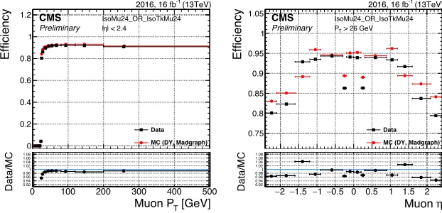
Figure 14.HLT-only trigger efficiency as a function of offline muonpTwith|η|<2.4 (left) and of offline muonη
withpT >25 GeV (right) for the OR of the HLT IsoMu24 and HLT IsoTkMu24. These two trigger paths require
a muon reconstructed online withpT >24 GeV as well as passing an isolation selection. The HLT-only efficiency
has been computed as the trigger efficiency for events passing the L1 trigger. [17]
[GeV]
T
Muon P
Efficiency
0 0.2 0.4 0.6 0.8 1 1.2
Data MC (DY, Madgraph)
(13TeV)
-1
2016, 16 fb
CMS
Preliminary IsoMu24_OR_IsoTkMu24|η| < 2.4
[GeV]
T
Muon P
0 100 200 300 400 500
Data/MC 0.920.94 0.96 0.981 1.02 1.04 1.06 1.08
η Muon
Efficiency
0.75 0.8 0.85 0.9 0.95 1 1.05
Data MC (DY, Madgraph)
(13TeV)
-1
2016, 16 fb
CMS
Preliminary IsoMu24_OR_IsoTkMu24PT > 26 GeV
η Muon 2
− −1.5 −1−0.5 0 0.5 1 1.5 2
Data/MC 0.920.94 0.96 0.981 1.02 1.04 1.06 1.08
Figure 15. Combined HLT and L1 trigger efficiency as a function of offline muonpT with|η|<2.4 (left) and
of offline muonηwithpT >25 GeV (right) for the OR of the HLT IsoMu24 and HLT IsoTkMu24. These two
trigger paths require a muon reconstructed online withpT >24 GeV as well as passing an isolation selection.
[17]
[2] CMS Collaboration, “CMS Technical Design Report for the Level-1 Trigger Upgrade,”
CERN-LHCC-2013-011, CMS-TDR-12, https://cds.cern.ch/record/706847
[3] CMS Collaboration, “Level-1 E/Gamma and Muon performance on 2017 data”,
CMS-DP-2017-024, https://cds.cern.ch/record/2273270
[4] CMS Collaboration, “Level 1 Tau trigger performance in 2016 data and VBF seeds at Level 1
trigger”, CMS-DP-2017-022, https://cds.cern.ch/record/2273268
[5] CMS Collaboration, “CMS L1 Calorimeter Trigger performance in 2016 data”,
[6] CMS Collaboration, “L1 muon trigger performance - ICHEP16 dataset”, CMS-DP-2016-050, https://cds.cern.ch/record/2202986
[7] CMS Collaboration, “Level-1 muon trigger performance in 2017 data and comparison with the legacy muon trigger system”, CMS-DP-2017-041, https://cds.cern.ch/record/2286327
[8] S.Donato, L.Rolandi, A.Rizzi, “Search for the Standard Model Higgs boson decaying to b quarks with the CMS experiment” CMS-TS-2017-008, CERN-THESIS-2017-059, https://cds.cern.ch/
record/2268298
[9] CMS Collaboration, https://twiki.cern.ch/twiki/bin/view/CMSPublic/HLTplotsCHEP2016
[10] CMS Collaboration, https://twiki.cern.ch/twiki/bin/view/CMSPublic/HLTplotsPixelUpgrade
[11] CMS Collaboration, https://twiki.cern.ch/twiki/bin/view/CMSPublic/HLTplotsFirst2017Data
[12] CMS Collaboration, “High Level Trigger Performance Plots for ICHEP2016” CMS-DP-2016/056, http://cms.cern.ch/iCMS/jsp/db_notes/notestable1.jsp?CMSNoteID=DP-2016/056
[13] CMS Collaboration, “Performance of online b tagging in proton-proton collisions at 13 TeV at the CMS experiment” CMS-DP-2017-011, http://cms.cern.ch/iCMS/jsp/db_notes/notestable1.jsp?
CMSNoteID=DP-2017/011
[14] CMS Collaboration, “Electron and photon performance in CMS with the full 2016 data sam-ple”, CMS-DP-2017-004, http://cms.cern.ch/iCMS/jsp/db_notes/notestable1.jsp?CMSNoteID=
DP-2017/004
[15] CMS Collaboration, “Tau trigger commissioning on first 2017 13 TeV data”, CMS-DP-2017/035, http://cms.cern.ch/iCMS/jsp/db_notes/notestable1.jsp?CMSNoteID=DP-2017/035
[16] CMS Collaboration, “Tau trigger performances on 2016 13 TeV data”, CMS-DP-2017/031, http: //cms.cern.ch/iCMS/jsp/db_notes/notestable1.jsp?CMSNoteID=DP-2017/031