Compiled visualization with IPI method for analysing of liquid liquid mixing process

Compiled visualization with IPI method for analysing of

liquid-liquid mixing process

Darina Jasikova1,*_{, Michal Kotek}1_{, Bohus Kysela}2_{, Radek Sulc}3_{, and Vaclav Kopecky}1

1_{Department of physical measurements, Institute for Nanomaterials, Advanced Technology and Innovation, Studentska 1402/2}

460 01 Liberec 1, Czech Republic

2_{Institute of Hydrodynamics AS CR, v. v. i., Pod Patankou 30/5, 166 12 Prague 6, Czech Republic}

3 _{Czech Technical University in Prague, Faculty of Mechanical Engineering, Department of Process Engineering, Technicka 4, 166 07}

Prague, Czech Republic

Abstract. The article deals with the research of mixing process using visualization techniques and IPI method. Characteristics of the size distribution and the evolution of two liquid-liquid phase’s disintegration were studied. A methodology has been proposed for visualization and image analysis of data acquired during the initial phase of the mixing process. IPI method was used for subsequent detailed study of the disintegrated droplets. The article describes advantages of usage of appropriate method, presents the limits of each method, and compares them.

1 Introduction

Mixing is a very important operation in chemical industry and process engineering. It represents more than sixty percent of all industrial processes. A huge amount of mass is mixed in vessels stirred by an impeller. Large agitated tanks with impellers are used in food industry, pharmacy, and also in mining industry, waste water treatment etc. The global trend in process optimization involves new technologies providing higher quality products with lower energy demands. Trend is to develop more efficient mixing equipment. The optimization of stirred vessel and impeller design is done with help of Computational Fluid Dynamics simulations. The importance of these simulations validation was in recent past overlooked. Today, we are returning again to verification and the value of experimental validation is increasing.

Modern CFD methods are dealing with prediction of drop size distributions and their dynamics. This parameter determines mixing process evolution. The drop breakage, coalescence rates and final droplet size distribution depends on geometry of vessel and impeller, agitation rate and physical properties of mixed phases. Kolmogorov [1] and Hinze [2] were the first, who derived a relation for the maximum drop diameter. The maximum drop size dmax is determined by external deforming forces and restoration forces. Kolmogorov found the relation between dmax and local rate of energy dissipation . The time evolution of drop size distribution is based on theory of breakage and coalescence functions. Though, physical background is well described the basic relations and boundary conditions have to be improved depending on actual setup. [3]

Separate branch of research is becoming a development of methods enabling experimental validation of CFD simulations. Basically, measurement methods can be divided in two groups: the first one is based on sampling procedure; the second one is based on ex-situ measurements. [4] The ex-situ measurements can be done on emulsion before it coalesces, or on stabilized emulsions. The first group of measurements can be run directly with the mixing process and gives information about its evolution. These methods are mostly based on optical principles. The advantages of optical observations are in their non-invasive character. The disadvantage is limitation in the measurable range of droplet sizes. Expected droplet size distribution is above units of micrometres in mixing process. It can also reach sub-millimetre sizes at very beginning. This range can be covered with automated imaging, light back-scattering, and ballistic imaging methods. The first investigation of two-phase breakups of liquid in air is dating to before 1904. [2] These researchers used short-flash photographs showing the breakup of drops. This simple method upgraded with industrial sensitive camera and powerful light source, and helps reveal initial instabilities, shape of bulks and disintegration of one phase in these days as well in past. Even, we refill the camera with magnifying lens system, for example long distance microscopy, the limits of imaging are in micrometre size of droplets. Especially, it is essential if we look at a larger area for statistical evaluation. [5]

lasers in 60‘s brought more sophisticated methods such as PDA, and ILIDS, or IPI. [6, 7]

Phase Doppler anemometry (PDA) is an extension of laser Doppler anemometry (LDA). It is single-point measurement method. We can provide size and velocity measurement using this technique. The extremely difficulty of this methods is based on its principle. It is a local measuring method, so if the mixing process develops rapidly, it requires fast traversing over investigated area. On the other hand PDA enables measurement of large scale of particle sizes (0 -300) um and their velocities. It is useful method for study of stabilized dispersions.

Interferometric Particle Imaging (ILIDS or IPI) was developed as the alternative to the PDA. ILIDS can provide instantaneous spatial distribution of particle diameter. The spatial pattern is generated by the interference of external reflection and direct refraction of the droplet that is placed in the laser sheet. The limits of this method are in the size of defocused image, when in denser systems particles interfere together. Deploying this method is appropriate when primary disintegration of liquid bulks has already occurred and disintegration of liquids leads to separated droplets in volume. This method gives results of long-term measurements for evaluation and validation final droplet size. It works very well on ranges of particle size (10 - 300) um.

The motivation of our research was finding way to describe evolution of the mixing process and droplets disintegration as well as the stable dispersion that reach units from millimetres to micrometres. We tried to follow droplet size and shape. We have compiled a visualization setup with knowledge of the limitations of above mentioned methods that enables record initial part of rough disintegration during mixing process and also further settling phase. We combined shadowgraph method using backlight and industrial camera with IPI camera setup and laser light. The connection of both methods and the comparison of the results can give us tool that can be applied on scaled model of stirrer vessel.

2 Experimental Methods

2.1 Stirred Vessel Setup

We designed the scaled model of stirred vessel with inner diameter of cylindrical tank D = 150 mm and height H=D, position C = 1/4H.

We also used scaled model of Rushton turbine impeller of size D1 = 37 mm, w= 10 mm, l = 12 mm and

t= 1 mm. The vessel was set with four baffles of width B/D=1/10, so was B = 15 mm fixed evenly around circumference of the vessel. The height of the liquid level was covered.

There was used degassed water as a working liquid (density ρ = 1000 kg.m3_{, dynamic viscosity μ = 1 mPa.s)}

under constant impeller speed 540 rpm. The volume of water was 2.65l.

The second phase was Rhodosil Oil 47V50 (density ρ = 959 kg.m3_{, dynamic viscosity μ = 50 mPa.s, and}

surface tension  = 20. 7 mN/m) injected directly into

the vessel. The volume of oil was set 1% of liquid volume, so we used 26 ml.

Fig. 1. Geometry of stirred vessel.

Fig. 2. Sketch of Rushton turbine impeller.

2.2 Shadowgraph Method

Suite. The intensity of light impacting the camera chip was manually set with the aperture. The back-lighting allowed the visualization of droplet shadows that appear as a black bounded object on white or light-grey background. Weakness in this conventional setup is in picture of drops that are out of camera focusing plane. These unfocused droplets move the statistics to higher values. The inverse mode of this setup enables capture light reflected on the surface of droplet. The droplets are seen as closed rings on the dark background. These rings appear only in focusing plane of the lens system. The rest of particles that are out of focus don’t have sufficient contrast and cannot be edged detected. The inversed setup turned out to be more advantageous for further image processing and analysis.

The capturing frequency was adapted to the evolution of emulsification process. It was set 0.5 Hz to obtain the initial phase and rough disintegration into separated droplets.

a) b)

c) d)

Fig. 3. Examples of records captured with shadowgraph method. a), and b) bulks of liquid at very beginning of mixing process; c) middle part with disintegration, d) stabilized disintegrated droplets of oil.

2.2.1 Image Processing

The image sequence was captured with frequency 0.5 Hz. The time of the record was set according to evolution of the process and last 140 sec. The image processing run in ImageJ open source software. The images were adjusted on brightness and contrast to eliminate unfocused and blurred droplets. The threshold function was used to remove dark background, highlight droplets and transform image to binary level. Next step of image preparation contained set of binary operation.

There was applied mathematical morphology closing operator. Closing operator enlarged foreground region and kept original boundary shape. We managed improve the closure of rings (drops) and repair it, where it was missing due uneven light reflection. The prepared rings could be filled with another morphology operator – filling holes.

Software ImageJ provide special function for particle detection and analysis. This function works by scanning the image until it finds the edge of an object. The object can be specified by the size of particle, and circularity. The circularity set in range 0.8-1.0 enables to remove non spherical particles, such as bulks of liquid or particles joined together due overlap in the focusing plane. This variable set is based on researchers’ experience, and an unhealthy setting may change the evaluation of statistical interpretation. We removed very small particles (noise due image processing) with setting the minimum area of particle to 10um2_.

It was quite a problem at beginning of the mixing; when the liquid was formed into bulks of non-spherical shape, and diameter above 1mm (see Fig. 3). Result of analysis was presented as Sauter Mean Diameter D[3,2].

Capture Image Record

Applied Closed and Filled function

Fig. 4. Results after application of sequence image processing method.

2.3 Interferometric Particle Imaging Method (IPI) The interferometric method of droplet sizing or interferometric particle imaging (IPI or ILIDS) can be attributed to the class of field optical investigation methods for two phase flows. One phase is liquid and second phase can be gas or liquid with different density, viscosity or immiscible liquid. It gives information about droplets is the whole chosen cross-section of the flow. That is great advantage of this method. The IPI can be apply to flow with lower densities of second phase and also requires optically transparent medium that enables light reflection and refraction.

The IPI method uses the distance between the fringes of interference pattern which is formed by light reflected and once refracted by a droplet to measure the droplet diameter. The fringe pattern is created by defocusing of camera. The level of defocused particle image is between 50 px and 120 px. There are mathematical suggestions, but proper correction depends on actual scene, and light conditions. The measurement system is based on laser, formed in the light sheet, and digital camera with defocused lens. The camera registers interference patterns from all droplets illuminated by the light sheet. Here comes the restriction by droplet concentration.

Other limitations come with the physical background of IPI method. There are set lower and upper limits of measured particle diameter for each experimental setup. The first limit relates to geometrical optics. The second limitation depends on actual setup, i.e. camera distance, objective aperture, collecting angle. These limits are reflected in the number of interference fringes. The minimum number of fringes and therefore measurable diameter is N=2. Such a pattern can be easily created by secondary reflection. Evaluation of such noise as a valid particle is incorrect. This reading is reflected by shifting the peak to the smallest particles in the resulting histogram. Limits for maximal size of particles are related to Nyquist theorem. There is set the minimum distance between fringes in interference pattern x=2px. [8, 9, 10]

The experimental setup for IPI technique is based on laser source and high-resolution camera. The simplest version doesn’t require two cameras, when velocity field calculation is not need. Here we used Nd:YAG pulse laser NewGemini, working on 532 nm with output energy of 80 mJ per pulse. The laser illuminated region of size (56 x 68) mm that was also set as investigated area. The laser sheet thickness was 3mm. The camera HiSense Neo with resolution (2560x2160) px and 12-bit dynamic range. This camera was fitted with an objective with a focal length 60 mm (f/2.8). The distance between laser sheet and camera was 800 mm. This experimental setup with scattering angle 60°, aperture diameter of 21.430 enables measurement of droplet diameter minimum 21.58 um and maximum 323.63 um.

We run IPI measurements every 5 minutes and there were captured 256 records in each run. Sampling frequency was set 10 Hz. The first run was set immediately after the injection of Rhodosil oil. Immediate creation of large bulks of oil drops disabled

measurement due huge light scattering. Emulsion started to be measurable after 8minutes of mixing, this correspond to shadowgraph method. Droplets are significantly separate and starting to have uniform distribution.

Analysis of results also contained image post processing procedures such as subtract of mean image to reduce scattered light, masking of objects and dark areas, and filters (edge detection, threshold).

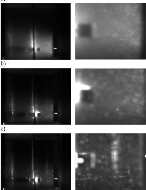
a)

b)

c)

Fig. 6. Camera view on mixing process. The focused picture of interference structure. a) blurred investigated area due scattered light from bulks of oil, b) phase of forming droplets, c) measurable medium with well separated droplets of uniform size.

3

Results and Discussion

The theoretical considerations of stirring on liquid-liquid dispersion include definition of Reynolds and Weber numbers. Reynolds number classifies the flow regime. We were at the stage of looking for a methodology for evaluation, so we could not afford the Re > 104_{. We}

needed to monitor the relatively slow start of the process so we adjusted the speed of rotation. The Reynold number calculated:

ܴ݁ ൌ ఘǤேǤ஽_ఓ మ (1)

where  is liquid density [kg.m3_{], µ is dynamic}

viscosity [Pa.s], N is stirrer rotational velocity (s-1_{), and}

D is diameter of the stirrer [m].

The Reynolds number was 20x103 _{in our case, so we}

The balance between break-up and coalescence of the droplets can be expressed by Weber number:

ܹ݁ ൌ ఘǤே_ఙమǤ஽య (2)

where  is interfacial tension [N/m].

Using Weber number we are able estimated dmax:

݀௠௔௫ൌ ͲǤͳʹͷǤ ܹ݁ି଴Ǥ଺Ǥ ܦ (3)

Predicted size of particle was calculated as 160 um. The calculation is based on the Weber number with exponent 0.6. The exponent itself is subject of optimization. It seems to be dependent on the uniqueness of the stirred mixture of liquids. We used this value to set the experiment, especially the IPI method’s range.

We measured the experiment with Rhodosil Oil in two separate runs. The mixing process was captured with shadowgraph method during its evaluation. The IPI method was applied after first 2 minutes of immeasurable stadium. Fig. 7 and 8 shows stable state 10 minutes after injection. Fig. 7 and 8 are comparable. We did this experiment to validate dataset measured with IPI technique using different method. There is seen difference on the level (20 - 40) um. The IPI histogram of oil droplet size contains characteristic values. This is due to shadowgraph method image processing. The lower limits were set during the Particle Analyse function. These limits reduced the population of droplets with this diameter. There is seen missing column in fig. 7. The visualization method can be improved with regard to the estimated process development. We were not sure about the development of the disintegration at this initial experimental setup. The optics of the visualization system has been chosen to hit large particles (above 1mm in diameter). We were interested in a larger evaluation area. We already know that the smallest droplets reach about 30 um. We choose optics that will allow greater magnification in the next step of research.

Fig. 7. Histogram of particle diameters of oil droplets evaluated from shadowgraph records in stabile part of dispersion.

We calculated Sauter Mean Diameter SMD for both measurements. This value is presented as volume

diameter D[3,2]. There is agreement for both measurements with different technique. The D[3,2] for shadowgraph method was 116,13um and D[3,2] for IPI method was 119,9um. The values differ in 3%. This error is award to methods. The second influence is uneven adhesion of larger oil bulk to vessel walls, baffles, and lid in unmeasurable amounts, which affects the overall viscosity of the liquid.

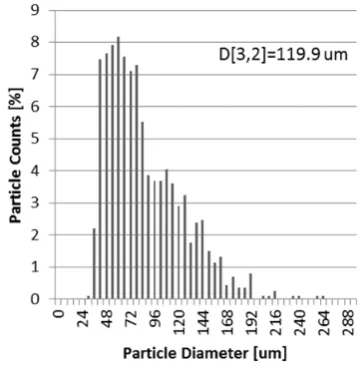
Fig. 8. Histogram of particle diameters of oil droplets evaluated from IPI method in stabile part of dispersion.

The finer histogram, see Fig. 9, represents detailed IPI graph. Previous interpretations of measured data by the IPI method were tailored to the occurrence of classes as set by the visualization method. The distribution in Fig. 9 is separated into finer steps. The IPI is more sensitive to the circular nature of the particles, and eliminates large particles outside the measurable range.

Evidence that the IPI method was set correctly is that it does not arise from the analysis of secondary interfering patterns. There is no false peak (phantom pattern) due to noise.

These evaluations show that in the stabile part of mixing process we can compare both methods and the results are not significantly different.

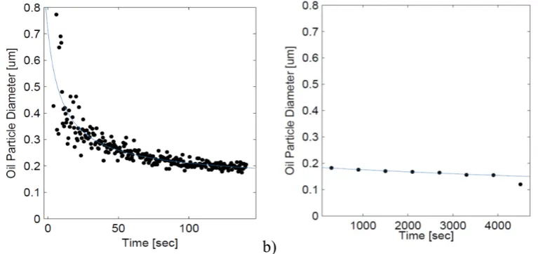
Comparison of the time course in figure 10 is combining results of both methods. The a) represents dataset results captured by shadowgraphy method. This part of chart fluently continues in part b). Part b) of Fig. 10 represents dataset measured by IPI method. Each dot in the figure 10 a) indicates the evaluation and average value AVG dimeter of the detected drops in one record. Dots in figure 10 b) means IPI statistic evaluation within a few minutes of 256 records collected with 10Hz

frequencies during 26 sec. The shadowgraphy scanning frequency was 0.5 Hz. Therefore, scattering of points is higher, because they are not statically averaged.

Smaller time sampling was more advantageous due to the rapid dispersion of the oil phase. This is a unit of seconds. While the staging phase of the process takes a few minutes. Once, we have tool for automated analysis the sampling frequency can be set higher. The upper limit for sampling frequency is the velocity of moving droplets.

a)

b)

Fig. 10. Evaluation of time evolution of mixing process – comparison of shadowgraph images and IPI method. a) Results of analysis of shadowgraph images – AVG diameters, b) IPI – AVG diameter statistics

It is required that the particle population in each image changes and the same particles are not measured several times.

The question is whether the gradual trend of decreasing of average particle diameter is due to progressive disintegration, or rather by settling of the bulk of liquids on the walls of the vessel, or separating them on the cover.

Each of these methods is suitable for study of different part of the dispersion process. The chosen method is complementary and directly related to the size distribution of the particles. To verify the accuracy of the methods, an overlay time window can be found in which it was possible to evaluate the size distribution of both methods (Figure 7, and 8)

It appears that the size stops significantly decreasing after 2 minutes of mixing, depending on evolution in time. It is possible, in this particular case (ratio 1% of volume), to mix two liquids in a given ratio to be stabilized in this time.

It has been shown that combining these two methods (visualization and IPI method) can include a comprehensive overview of the development and stabilization of the mixing process of two liquids.

Acknowledgment

Authors gratefully thank to the support of Grant Agency of the Czech Republic (GA ČR) 16-20175S Local turbulent energy dissipation rate in dispersion systems, and LO1201 co-funding from the Ministry of Education, Youth and Sports as part of targeted support from the „National Programme for Sustainability I".

References

1. A.N. Kolmogorov, Dokl.Akad.Nauk SSSR, 6 (1949) 2. J. O. Hinze, A.I.Ch.E. Journal, 1,3 (1955)

3. P. Ditl, F. Rieger, Chemical Engineering Progress, 102 (2006)

4. A. Khalil, Chem.Eng.J., 165 (2010)

5. T. Kawaguchi, Meas. Sci. Technol., 13 (2002) 6. F. Pereira, Meas. Sci. Technol., 15 (2004) 7. Ch. Dunker, Meas. Sci. Technol., 27 (2016) 8. N. Semidetnov, Meas. Sci. Technol., 15 (2004) 9. M. Itoh, Optical Review, 5 (1998)