ABSTRACT
Shedd, Justin M. - Remote Sensing Procedures to Update Forested Geospatial Datasets
after a Landscape Altering Event
The creation of accurate geospatial datasets like vegetation and fire fuel loads is a time consuming effort and these datasets are routinely used by resource managers. Therefore the accuracy of these datasets is vital. Vegetation and fire fuel load datasets often represent a dynamic landscape and landscape altering events such as a wildland fire or a hurricane can drastically change that landscape. The goal of this research is to investigate the use of automated change detection techniques that can not only indicate areas of change but also quantify the magnitude of change that occurred as well.
Hurricane Isabel did extensive damage to the forest landscapes of central Virginia in September of 2003, specifically Petersburg National Battlefield. The Rocky Top Fire
occurred in July of 2002 in Shenandoah National Park, resulting in a mosaic pattern of burns, covering roughly 1500 acres.
post-event fuel load datasets using the FARSITE model, thereby cataloging the potential need for vegetation and fuel load updates.
Remote Sensing Procedures to Update Forested Geospatial Datasets
after a Landscape Altering Event
by
Justin McEachern Shedd
A thesis submitted to the Graduate Faculty of North Carolina State University
In partial fulfillment of the Requirements for the degree of
Master of Science In
Natural Resource
Raleigh, NC 2006 Approved by:
________________________ ________________________ Dr. Heather Cheshire Dr. Stacy Nelson
ii DEDICATION
BIOGRAPHY
The author grew up in Virginia Beach, Virginia and is a graduate of UNC-Chapel Hill with a bachelor’s degree in Geography. After graduation he worked at several National Parks across the United States; working as a seasonal park ranger for the U.S. National Park Service in Utah, Oregon, Wyoming and North Carolina, specifically at Arches, Crater Lake, and Grand Teton National Parks, and the Blue Ridge Parkway. His strong interest in natural resource issues, remote sensing and knowledge of Geographic Information Systems led him back to North Carolina State University, specifically the Center for Earth Observation. Awarded a Teaching and Research Assistantship has afforded him numerous opportunities; from the development of assignments and web-pages to the various National Park Service projects, in turn preparing him for a future GIS career.
iv
ACKNOWLEDGMENTS
I would like to thank my committee members Dr. Hugh Devine, Dr. Heather
Cheshire, and Dr. Stacy Nelson for not only helping me through my arduous journey that has culminated in my thesis, but for their dedication to teaching. Their knowledge and personal interest has been evident in the several classes I have taken. I would like to extend a thank you to several former and current employees of the Center for Earth Observation: Linda Babcock, Kris Callahan, Beth Eastman, Bill Millinor, and Bill Slocumb as well as several students; specifically Barry Hester, Dr. Frank Koch and believe it or not Tom Colson.
Furthermore, thank you Melissa Foder and especially KellyAnn Gorman of
Shenandoah National Park, as you were an excellent source of fire-related information and insight. Thank you Tim Blumenschine and Larry Newkirk of Petersburg National Battlefield for answering all my questions and being my tour guide.
To my field crew: Kris, Millinor and Jill Stephens, without you I’d still be counting and identifying twigs and Dan Hurlbert, for letting me use your house, it helped immensely – Thank You.
TABLE OF CONTENTS
List of Figures ... ix
List of Tables ... xi
1. Introduction...1
2. Literature Review...3
2.1 Forest Fuels...3
2.1.1 Fuel Description...3
2.1.2 Fuel Mapping...5
2.1.3 Measuring Fuels...8
2.1.4 Fuel Models ...9
2.1.5 Fire Behavior Models ...12
2.2 Remote Sensing ...13
2.2.1 Remotely Sensed Imagery ...13
2.2.1a Satellite...13
2.2.1b Digital Aerial Photography...14
2.3 Change Detection...15
2.3.1a Kauth-Thomas...16
2.3.1b Normalized Differenced Vegetation Index...17
2.3.1c Normalized Burn Ratio ...18
2.3.2 Automated Feature Extraction ...20
2.3.2a eCognition...21
2.3.2b VLS Feature Analyst...22
2.4 Agents of Change...24
2.4.1a Hurricanes and Wind Damage upon Forests...24
2.4.1b Mapping Wind Induced Forest Damage...25
vi
3. Objectives ...32
4. Study Areas...33
4.1 Petersburg National Battlefield...33
4.2 Shenandoah National Park...35
5. Methodology...37
5.1 Visual Learning Systems Feature Analyst...37
5.1.1 Data and Initial Classification Attempts...37
5.1.2 Parameters of Feature Analyst ...39
5.1.2a Training Sites ...39
5.1.2b PatternRecognizers ...40
5.1.2c Other User Defined Parameters ...42
5.1.2d True Color versus Color Infrared...43
5.1.3 Mapping Downed Woody Debris ...44
5.1.4 Additional Sections of Petersburg National Battlefield...49
5.1.5 Construction of Forest Damage Polygons ...51
5.1.6 Creation of Fuel Load Datasets...54
5.1.7 Preparation for Field Work ...55
5.1.8a Field Work – Accuracy of Feature Analyst ...56
5.1.8b Field Work – Fuel Data Collection...56
5.1.8c Field Work - Modification of Brown’s Transect ...58
5.1.8d Field Work – Forest Damaged Areas...59
5.1.9 Fuel Load Calculation...59
5.1.10 Post Processing ...60
5.2 Remote Sensing Landsat...62
5.2.1 Data Type and Availability...62
5.2.2 Pre-Processing...62
5.2.3 Data Transformations and Spectral Enhancements ...64
5.2.3a Normalized Differenced Vegetation Index ...64
5.2.3b Tasseled Cap ...66
5.2.4 Comparison of Data Transformations...69
5.2.5 Preparation for Field Work ...70
5.2.6 SHEN Field Work...71
5.2.7 Fuel Load Calculation...72
5.2.8 Post Processing ...73
5.3 Field Work Recap ...73
5.4 Creation of FARSITE layers...74
6. Results...80
6.1 Petersburg ...80
6.1.1 PETE Results ...80
6.1.2 Feature Analyst Results ...80
6.1.3 Fuel Loading Calculation...81
6.1.4 Forest Damage Polygons ...83
6.1.5a Formation of New Spatial Datasets - Fuel Model...86
6.1.5b Formation of New Spatial Datasets – Vegetation...87
6.2 Shenandoah ...88
6.2.1 SHEN Results ...88
6.2.2 Classification Comparison...88
6.2.3 Fuel Loading Calculation of dNBR Results ...90
6.2.4 Qualitative Measure of Vegetation ...95
viii
7.1.1 The use of Digital Aerial Photography ...113
7.1.2 Feature Analyst ...113
7.1.3 PETE – Updating Spatial Datasets ...114
7.1.4 Determining Forest Damaged Areas...116
7.2.1 Normalized Burn Ratio...117
7.2.2 SHEN – Updating Spatial Datasets...118
7.2.3 FARSITE and Canopy Cover ...119
8 Conclusions...121
References...124
Appendices...131
Appendix A. dNBR Classification Guideline...132
Appendix B. Composite Burn Index...133
Appendix C. PETE Fuel Loading Values ...134
Appendix D. PETE Updated Fuel Model Spatial Dataset ...146
Appendix E. PETE Updated Vegetation Spatial Dataset...148
Appendix F. SHEN NDVI Classification ...150
Appendix G. SHEN Tasseled Cap Classification...151
Appendix H. SHEN dNBR Classification ...152
Appendix I. SHEN Fuel Loading Values ...153
Appendix J. SHEN Fuel Loading across dNBR classification ...162
Appendix K. SHEN Updated Fuel Model Spatial Dataset ...164
LIST OF FIGURES
Figure 1. Map of Petersburg National Battlefield...34
Figure 2. Map of Shenandoah National Park...36
Figure 3. Example of Unsupervised Classification using 40 classes...38
Figure 4. Example of NDVI Classification...39
Figure 5. Example of Training Sites...40
Figure 6. Foveal, Bulls Eye 1 and Bulls Eye 4 Pattern Recognizers ...41
Figure 7. Example of classification results using different pattern recognizers ...42
Figure 8. Example of more specialized classification per iteration ...42
Figure 9. Example of Feature Analyst passes for one iteration ...46
Figure 10. Example of Feature Analyst mapped downed woody debris ...51
Figure 11. Pictures of downed woody debris not detached from its origin ...52
Figure 12. Example of forest damaged forest polygons ...55
Figure 13. NCSU-CEO Microsoft Access Database ...58
Figure 14. Location of plots for PETE, Western Front...60
Figure 15. Location of plots for PETE, Eastern Front...61
Figure 16. Location of plots for PETE, Fort Gregg...61
Figure 17. Location of CBI plots ...69
Figure 18. Location of plots for SHEN...74
Figure 19. Fuel Loading for 1-Hour fuels of PETE...84
Figure 20. Fuel Loading for 10-Hour fuels of PETE...84
Figure 21. Fuel Loading for 100-Hour fuels of PETE...85
Figure 22. Fuel Loading for 1000-Hour fuels of PETE...85
Figure 23. Acreage of Rocky Top Fire per dNBR classification...93
Figure 24. Fuel Loading for Plots located in dNBR Class 2 ...93
Figure 25. Fuel Loading for Plots located in dNBR Class 3 ... 94
x
Figure 30. FARSITE, PETE All Rate of Spread Simulation Results ...106
Figure 31. FARSITE, PETE All Fire Line Intensity Simulation Results ...107
Figure 32. FARSITE, SHEN All Perimeters ...108
Figure 33. FARSITE, SHEN All Flame Length Simulation Results...109
Figure 34. FARSITE, SHEN All Rate of Spread Simulation Results ...110
Figure 35. FARSITE, SHEN All Fire Line Intensity Simulation Results ...111
LIST OF TABLES
Table 1. PETE Percent covered/Assigned Fuel Model...54
Table 2. Comparison of Classifications with CBI data...70
Table 3. Feature Analyst Error Matrix...81
Table 4. dNBR Classification Error Matrix...90
Table 5. PETE, FARSITE area variation...99
1 Introduction:
Historically, wildland fire has played a significant role in the Eastern
United States. Native Americans (prior to 1600s) are believed to have burned grasslands and forests to encourage wild game and desired crops (Frost 1998). Likewise, early European settlers (1800s) actively burned to clear land for crops and livestock (Pyne 1982). More recently, after decades of successful suppression, wildland fires nationally have been reduced in frequency but have increased in severity and size (National Interagency Fire Center Website, http://www.nifc.gov). In addition, as described by Cohen and Sutherland (1997), residential and business development has been increasing in areas adjacent to forested regions, giving rise to considerable threats to both lives and property in the Wildland Urban Interface (WUI). The WUI creates an environment in which a fire can spread easily between vegetation fuels and structures. The build-up of forest fuel loads, from a lack of wildland fire, coupled with the encroachment of the WUI has led to more costly and deadly fires.
National Park Service fire management plans, call for the pre-suppression management of forest fuels (http://www.nps.gov/fire/fire/fir_wildland.html). Proper management (pre-suppression and suppression) of forest fuels requires explicit knowledge about their type, continuity, and spatial distribution. Geospatial datasets, specifically vegetation and fuel loads, enable land management officers to plan and implement various tactics to reduce the overall fuel load as well as allowing for the allocation of vital resources in the event of a wildland fire.
knowledge of the situation they will be encountering. However, a GIS is useful only with accurate data. Forest fuels do not cause a fire to start; they do however have dramatic effects on the characteristics of a fire. Fuels are dynamic, always in a state of flux, due to influences of moisture and rates of decay, as well as changes in fuel loading and
arrangement (Pyne 1996). Therefore, the accuracy of the geospatial datasets that describe these fuels is vital and the need to update them, especially after a landscape altering event such as a hurricane or a wildland fire, is imperative.
2 Literature Review:
The following literature review examines various aspects of updating geospatial datasets after a landscape-altering event has occurred. Forest fuels and their importance in the ecosystem and on wildland fire are discussed, along with various methods of measuring and mapping fuel loads. Studies of mapped wind-induced damage occurring in forested landscapes are also reviewed. In addition, automated feature extraction and pixel based classification methods and studies utilizing various remote sensing data transformation methods to record fuel load and vegetation change after a wildland fire are compared.
2.1 Forest Fuels
2.1.1 Fuel Description
further divided into several categories: fine woody debris (sticks less than 3 inches in diameter), coarse woody debris (sticks greater than 3 inches in diameter), duff (layer of distinguishable organic matter on top of soil), and litter (loose leaves, twigs and pine cones on top of duff). Live fuels consist of biomass such as grasses, shrubs, saplings and trees.
Fuels are also described as hour fuels, e.g., 1-, 10-, 100-, and 1000-hour fuels. The moisture content of a fuel is regulated by environmental conditions such as air temperature, humidity, and windspeed (Burgan and Rothermel, 1986). The hour classification represents the time required for a fuel’s moisture content to reach equilibrium (with current atmospheric conditions) and is determined by the fuel’s
diameter. 1-Hour fuels measure less than 0.25 inches in diameter, 10-Hour Fuels are 0.25 to 1 inch in diameter, 100-Hour fuels are 1 to 3 inches in diameter and 1000-Hour fuels account for any downed woody debris over 3 inches in diameter (Burgan and Rothermel, 1986, Brown 1974, and Anderson 1982).
the main fire. Identifying and mapping areas with an abundance of CWD is important because it enables land managers to quickly access and mitigate potentially high fire risk areas. Therefore, the existence of an accurate spatial data layer representing fuel loads is one of the most important pieces of information utilized by a land manager.
2.1.2 Fuel Mapping
Early fuel mapping focus was on the rate of spread of a fire versus the initial attack response to the fire, with other projects focusing on how difficult a fire would be to suppress (Sandberg et al., 2001). Both of these approaches had little to do with
characterizing the actual fuel type or load, but instead focused on mapping the fire’s threat (to an area) or time till complete suppression. Early wildland fire research focused on fire fighter movement (personnel and equipment) and their ability to suppress the advancing front of a fire. As wildland fire research increased, knowledge of fuel characteristics and behavior has increased, enabling the creation of maps indicting the different forest fuels.
Regional or state level fuel maps allow researchers and planners to focus their efforts on reducing threats to homes in the Wildland Urban Interface. For example, Colorado State Forest Service, in their Wildland Urban Interface Hazard – Risk
Assessment Project, created maps to indicate hazards determined by overlaying natural resource (slope, fuels, aspect, etc.) and infrastructure (roads, population, homes, etc.) data layers (http://www.colostate.edu/Depts/CSFS/). The state of California’s Fire and
Resource Protection Division of the Forestry and Fire Protection Department had a similar project that involved overlaying a weighted fuels data layer and other environmental data layers to construct an at-risk data layer
(http://frap.cdf.ca.gov/projects/wui/). Both of these projects had a spatial resolution of one mile, designed for fire hazard comparisons between counties and areas of the state, not to determine wildand fire threats to individual homes.
Landscape or large-scaled fuel maps enable local land managers to map fuels of locations of interest at a smaller resolution. At Yosemite National Park, researchers used Landsat satellite imagery to delineate different types of forest fuels to give park fire management personnel a valuable tool for combating wildland fires (Van Wagtendonk and Root, 2000).
remotely sensed data, field reconnaissance is not used often today, but it was essential to early fuel mapping projects.
Direct mapping refers to the mapping of fuels using remotely sensed data, such as satellite imagery or aerial photography. Predominantly utilized in national and regional scaled fuel mapping projects, direct mapping projects utilize Leaf Area Index (LAI) (Jordan, 1969) or the Normalized Differenced Vegetation Index (NDVI) technique (Rouse et al., 1973). LAI refers to the measuring of the visible and near infrared energy reflected by vegetation. LAI provides information on the structure of the plant canopy, as well as expressing how much surface area is covered by green foliage relative to total land surface area. NDVI is calculated from the visible and near-infrared (NIR) light reflected by vegetation.
The biophysical modeling approach uses direct and indirect environmental gradients, such as climate, topography and landuse history, to map fuels. Biophysical modeling employs ecosystem models that quantify those gradients across a particular landscape (Keane, et al., 2001). At Glacier National Park a biophysical model using different topographic and vegetation layers was used to create a fuelbed spatial dataset (Kessell, 1979). While extensive amounts of data and statistical analyses are required, the resulting classification can be updated as conditions change. However, these datasets tend to express the potential vegetation of an area, not the actual vegetation found (Keane et al, 2001).
dataset. With most satellite sensors designed to discriminate different vegetation types, this approach is popular because of its accuracy and “two-for-one” mapping approach. Two datasets (vegetation and fuels) are created from a single purchase of remotely sensed data, making this approach cost effective and timely. This is the approach that North Carolina State University’s Center for Earth Observation (NCSU-CEO) followed when creating vegetation and fuel load spatial datasets for the North East Region of the National Park Service (NPS). Following a procedure developed by Millinor (2001) vegetation datasets were delineated from aerial photomosaics. Smith (2003) developed a crosswalk that allowed for the creation of a fuel load (based on the original 13 fuel models) spatial dataset relative to the type of vegetation mapped.
2.1.3 Measuring Fuels
Just as there are several approaches to mapping fuel loads; there are several methods upon which forest fuels are actually measured or quantified. The following section will discuss methods of measuring forest fuels as well as introduce the use of fuel load models that are data inputs into fire behavior computer models that simulate fire spread.
size class in tons per acre. The National Park Service (NPS) uses this method of data collection when monitoring vegetation and pre- and post-burn fire plots.
Qualitative fuel measures are done to record the fuel complex (arrangement and load type) of the plot; rather than a quantifiable measure of vegetation (Burgan and Rothermel 1984). Burgan and Rothermel developed an extensive list of field
measurements in order to capture an accurate representation of the vegetation and fuel complex found in the plot. Information such as: grass type and height, shrub type and height, and tree type and height are collected along with other non-tallied observations based on categories (e.g. waxy or oily leaves, litter source, litter compactness, bulk density, grass type, etc.). Numerous studies have used these qualitative measurements when creating custom fuel models for use in fire behavior models.
The difficulties of fuel bed data collection led to the development of standard fuel characterizations or fire fuel models (Rothermel 1972, Albini 1976, and Scott and Burgan 2005) and guides to facilitate assigning these fuel models (Anderson 1982, Scott and Burgan 2005).
2.1.4 Fuel Models
categories: Grass (Fuel Model 1, 2, and 3), Shrub (Fuel Model 4, 5, 6, and 7), Timber (Fuel Model 8, 9, and 10) and Logging Slash (Fuel Model 11, 12, and 13). Each category has different parameters (fuel particle size and load) that affect a fire’s rate of spread and intensity. Furthermore, within each category fuel models have additional parameters (surface area to volume, moisture of extinction, heat content, and others) that determine the characteristics of the simulated fire. For each of the fuel models an example
were rather inaccurate for other purposes such as, prescribed fire, wildland fire use during off-peak seasons and conditions, and simulating the effects of fuel treatments on fire behavior. Joe Scott and Robert Burgan (2005) developed 49 “new” fuel models along with a guide, similar to Anderson’s, to assist in assigning fuel models to landscapes. These new fuel models offer a marked improvement for fire behavior predictions outside peak fire season and in other areas of the United States other than the west.
The Fuel Characteristic Classification (FCC) system developed by the Fire and Environmental Research Applications team of the United States Department of
Agriculture, Forest Service Pacific Northwest Research Team provides a more in-depth characterization of fuelbeds (http://www.fs.fed.us/pnw/fera/fccs/). The FCC system uses fuelbed descriptions or “prototypes” which are based on; the quality of the fuel present and the abundance of fuels. Additional factors affecting the fuel complex, such as: vegetation form, structure class, and agent of change (e.g. disease, insect infestation) are input parameters used to create individual prototypes. All of these factors go into calculating total fuel loading and other parameters used by fire behavior models (Harrington, 2005). Unfortunately the FCC system has not yet developed its own fire behavior model (expected completion winter 2005) and has not been incorporated into any fire behavior model in current use.
2.1.5 Fire Behavior Models
There are several fire behavior models that rely on Rothermel’s fire spread model (Rothermel 1972). One such fire behavior model is FARSITE (Fire Area Simulator). Developed by Dr. Mark Finney, FARSITE is used by many federal land management agencies including the NPS. FARSITE is often used in a decision support system allowing land managers to make informed decisions based on the best available
information. As required by the NPS, each park must have a fire management plan; this plan provides specific details and operational procedures in case of a wildland forest fire. FARSITE is based on Huygen’s Principle that states that rate and spread directions of the fire are based on elliptical transformations (Finney 1998, 2004). These ellipses,
representing fire spread, are determined by wind speed, slope of the landscape and characteristics of the fuelbed. One of several input data layers required by FARSITE is a data layer that represents the fire fuel models. Currently the original 13 fuel models, the new 49 fuel models, and custom made fuel models can be input into FARSITE. Five spatial data layers are required by FARSITE in order to create a simulation; slope, aspect, elevation, fuel model, and canopy cover. Of those data inputs, fuel model is highly subjective, as it is determined by one or several professionals, and not necessarily by field measurements.
FARSITE will be used to validate the resulting classifications of the
2.2 Remote Sensing
2.2.1 Remotely Sensed Imagery
As mentioned earlier, indirect mapping using remotely sensed imagery is a cost-effective and timely approach to classifying vegetation; from which fire fuel model datasets can be created. The use of remotely sensed imagery and the various remote sensing techniques used to create geospatial datasets has increased dramatically over the recent decades (Blaschke 2000). Competition between an increasing number of
government and private satellites has lead to the reduction in cost, and increase in resolution of satellite imagery. Furthermore, the reduction in production time and cost coupled with an increase in spatial resolution, has led to the dramatic increase in the use of digital aerial photography as well (McGarigle, 1997 http://www.govtech.net).
2.2.1a Satellite Imagery
Depending on the requirements and desired outputs of a project there may be several types of imagery available. The Landsat Thematic Mapper (TM) sensor despite its relatively low spatial resolution (30mx30m) collects seven bands of spectral data. Landsat TM imagery has been used in countless change detection studies in both multi-image and single multi-image analyses (Lu 2004). With four of the seven bands recording in the infrared range, Landsat TM imagery is an excellent discriminator of vegetation (Lillesand et al., 2004).
accuracies have been solved, new problems have arisen, for example, the occurrence of a mixed pixel or “mixel.” A mixel denotes a pixel in which multiple classification (road, grass, forest) classes are contained. Merely increasing the spatial resolution of an image does not solve this problem; it creates new mixed pixels (Blaschke, 2000). Another issue is an inability to classify or map features easily discernable to the naked eye. The spatial resolution of aerial and satellite imagery has become so great that the importance of measuring a single pixel has given way to the power of detecting groups of pixels. In past studies, researchers focused on pixel by pixel analysis of an image to delineate or highlight a real world feature that was large in size, such as a shoreline or land cover type (White and Asmar, 1999). With the availability of high resolution remotely sensed data not only can large features like shorelines and landcover be delineated more accurately, but smaller features like homes (Al-Khudhairy, 2005) and streams (Zhang, 2000) can be delineated. Data classification techniques utilizing high resolution imagery focus on indicating features based on spatial patterns rather than on classifying a pixel by a range of spectral values.
2.2.1b Digital Aerial Photography
Digital photography relies on electronics rather than chemistry to capture and process images. The greatest benefit of digitally acquired aerial photographs is the quick turn around time and lower cost, all the while maintaining the overall quality of the image. Overall, the benefits (adjustable footprint of picture, immediate viewing of imagery allowing for instant quality control, simultaneously capture of true color and false color imagery, reduction in turn around time and production cost, etc.), (McGarigle, 1997 http://govtech.net) of digital aerial photography make it a valid choice of remotely sensed imagery for use in indicating areas of change.
2.3 Change Detection
In addition to the increase in available remotely sensed data like digital aerial photography and Landsat TM satellite data, the number of data enhancements or transformations used to classify these images has increased as well. Indicating features or areas of interest is important when maintaining the accuracy of spatial datasets. Automated Feature Extraction (AFE), specifically its ability to indicate areas of change by mapping real-world features like downed trees, with the resulting classifications being used to create updated geospatial datasets, will be discussed in the following section. In addition, change detection provides the foundation for a better understanding of
interactions between human and natural resource processes. This is especially of interest to land managers along the Eastern US as human development encroaches on forested landscapes. Not only does human development pose an increased risk to wildland fire, but landscapes altered by wildland fire need to be monitored to ensure further
several data transformations that can not only indicate but quantify change resulting from a wildland fire.
2.3.1a Kauth Thomas Data Transformation
Wildland forest fires modify biophysical properties in vegetation and in the various soil horizons (Patterson and Yool, 1998). Remote sensing data expresses these changes in terms of brightness, greenness, and wetness; which can be detected by the Kauth-Thomas or Tasseled Cap data transformation (Jenson, 2000). Initially created utilizing the Landsat Multi-Spectral Scanner (MSS) 4 band sensor (Kauth and Thomas, 1976), Tasseled Cap was modified for Landsat TM data utilizing 6 bands of spectral data (Crist and Cicone, 1984). Tasseled Cap data transformation rotates the spectral data so that they are shown in three dimensions representing brightness, greenness and wetness. The brightness indicator is a sum of all six TM bands. Greenness contrasts the sum of the visible and NIR bands. Wetness contrasts the sum of the visible and NIR by the sum of the longer wavelength bands.
not upon only vegetation, but across the entire landscape. Soils are typically only
blackened during cooler less intense fires, thus changing their brightness level (Pyne et al 1996). Canopy fires are typically associated with more severe burn events. With the overstory effectively removed, moisture in the form of humidity once captured by the forest canopy is no longer present. Fires of higher severity alter soil properties causing them to become water repelling (hydrophobic), causing environmental degradation in the form of mass wasting. Furthermore, in a study that mapped different levels of burn severity, the Tasseled Cap classification, when compared to the Intensity Hue Saturation (IHS) data transformation, was more accurate in its ability to detect varying levels of fire severity (Won, K. and J. Im, 2001). IHS can detect changes in brightness and greenness like Tasseled Cap but is unable to detect changes found on the wetness dimension. Instead of spectral values the IHS transformation uses the red-green-blue color
composites of various band combinations to detect changes in multi-temporal analyses (Koustsias et al., 2000). Images are classified based on their intensity, i.e. brightness or dullness of a color, hue, i.e., the dominant wavelength (color) and saturation, i.e., the purity of the color.
2.3.1b Normalized Differenced Vegetation Index
is also widely used as an indicator of forest canopy structure and percent cover. NDVI compares the differences between visible reflectance values (TM Band 3) and near infrared (TM Band 4). When using NDVI as an indicator of a fire’s severity, attention is paid to the reflectance values associated with physiological damage. In a healthy
ecosystem NIR wavelength reflectance is high, whereas in an ecosystem under stress as after a fire, a lower NIR wavelength reflectance is to be expected (Rogan and Yool, 2001). Studies along the Mediterranean Coast of Spain have shown that using a multi-temporal NDVI image results in both a better fire perimeter detection and an accurate fire intensity classification (Viedma et al., 1997, Garcia-Haro, 2001). Vegetation indices are not without their problems, as NDVI classifications are known to become “saturated,” meaning unable to discern areas of moderate to high levels of vegetation (Lillesand et al., 2004) and has been found to produce variable results dependent upon different cover types (Bonan, 1993), soil brightness and color (Rogan and Yool, 2001, Jensen 2000). Finally, there may be concerns with the output classifications indicating and categorizing surface burns that occur beneath a forest canopy (Major et al., 1990 and White et al., 1996) as the output pixel values are often saturated and do not indicate burned areas.
2.3.1c Normalized Burn Ratio
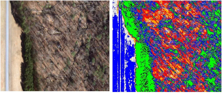
(VanWagtendonk et al., 2004) of burn severity in the field of remote sensing. The ratio uses multi-temporal differencing to enhance the contrast from a pre- and post-fire scene, creating a differenced NBR (dNBR) classification. dNBR is based on the premise that post fire reflectance for NIR band 4 decreases when compared to a pre-fire scene, while the MIR band 7 (indicating dryness in soil and vegetation) increases in a post-fire image (Key and Benson, 2002). When processing the dNBR data transformation, pre- and post-Landsat imagery acquired approximately during the same time of the year, preferably in the spring, should be used for analysis. This ensures that the images being contrasted represent land cover in the same physiological state, as vegetation reflects more IR wavelengths in the fall than in the spring. This will reduce the variation seen between images not associated with the burn event.
In 2000, from May 9th to November 14th, the Outlet Fire burned 13,000 acres along the Northern Rim at the Grand Canyon National Park. Researchers compared pre- and post-fire NBR and NDVI classifications in the hopes of mapping the fire’s severity upon the natural environment (Bertolette and Spotskey, 2001). The dNBR image was created from Landsat 7 imagery, while the NDVI image was created using Spot 4 imagery. Both images expressed wide ranges of spectral vales, but the NBR image provided the most discriminating and sensitive classification of burn severity despite a coarser resolution.
In 2001, the dNBR technique was used to classify burn intensities of the Hoover fire, a 7000 acre wildland fire occurring in Yosemite National Park. The output
classification using Landsat 7 Enhanced Thematic Mapper (ETM) imagery was
hyperspectral sensor. Despite a coarser spectral resolution when compared to the AVIRIS sensor, these results validated the use of Landsat Bands 4 and 7 to quantify a fire’s severity, as the Landsat imagery provided more accurate results than the AVIRIS imagery when ground-truthed (Van Wagtendonk et al., 2004).
NBR’s creators (Key and Benson, 1999) consider the pre- and post-fire image differences to indicate and enable the quantification of change caused by a fire, i.e., the levels of burn severity, not burn intensity. A fire may be of low intensity (flame height, heat, etc.), but of high severity because the fire consumes what little vegetation that did exist. This distinction is stressed to clearly differentiate between fire intensity and fire (or burn) severity (Parson, 2002). In addition to clarifying the type of indicator the dNBR transformation is, the authors developed a ground truthing technique called the Composite Burn Index (CBI). The collection of CBI field data in “initial” and “extended assessments” (Key and Benson, 2004) allowed researchers to adjust their early
classification system based on real fire-induced landscapes, leading to their guidelines followed today (Appendix A). The CBI will be discussed in more detail in section 2.4.2c.
2.3.2 Automated Feature Extraction
studies in which Automated Feature Extraction (AFE) is being utilized, e.g., from detecting structurally damaged homes (Al-Khudhairy, 2005) to detecting ships (Willhauck, 2005). Specifically in the realm of natural resources the power and capability of AFE techniques are being realized in research endeavors such as stream mapping (Dillabaugh, 2002) and mapping windthrown damage to forests (Jackson, 2000, Frannon, 2001 and Schwarz, 2003).
Many forms of AFE (image segmentation, object-oriented, contextual) exist (Blaschke, 2000) from edge-based systems to region-based systems, all have the same basic idea; neighboring pixels are related to each other and can therefore be clustered together. Until 2000, most image segmentation involved singular research efforts, manipulated to fit the local area or circumstance. There were no computer software packages with the ability of image segmentation available to the general public. In 2000, Definiens of Munich, Germany, launched eCognition, packaging a robust AFE tool that was transportable to all environments. Then Visual Learning System of Missoula, Montana, introduced Feature Analyst in 2001, packaging their version of an AFE in a graphical user interface. The use and successes of both software products are described on their respected websites (http://www.definiens-imaging.com/ and
http://www.featureanalyst.com/). In the following sections natural resource projects utilizing these software programs will be discussed.
2.3.2a eCognition
repeated at several scales. Beginning with a single pixel, groups of homogeneous pixels are merged together forming a series of segmented areas across an entire image. This process is repeated at a coarser scale to group the least dissimilar segments together.
eCognition was used in a study (Laliberte, 2004) to map shrub encroachment in southern New Mexico. Using 11 aerial photographs taken between 1937 and 1996 along with a Quickbird satellite image acquired in 2003, shrub encroachment resulting from years of fire suppression was mapped. Utilizing the fractal net evolution approach employed by eCognition, the images were segmented based on three attributes; shape, color, and scale. User defined parameters determined the break points that put pixels in one or another region. Beginning with a single pixel a region continues to grow,
acquiring new pixels until the smallest growth does not meet the threshold defined by the user. Researchers were not only able to track the increase in shrub growth over time, but could determine in which time period shrub growth increased the most.
2.3.2b VLS Feature Analyst
incorrect and correct areas are identified and the process is run again. This hierarchal process can be repeated until desirable results are met as defined by the user.
The United States Forest Service utilized Feature Analyst in a recent mapping effort (Vanderzanden, 2002). Using Quickbird and Landsat TM remotely sensed data, 65 square kilometers of the Tongass National Forest, in Alaska, were delineated into non-forested, deciduous, mixed, and coniferous forest classes, with forest classes further segmented based on their crown closure and tree size. Three classification
methodologies were explored; Feature Analyst using bands 2, 3, and 4 of a Quickbird image, a minimum variance texture filter (Woodcock and Ryherd, 1996) using Landsat TM imagery, and a supervised classification utilizing Landsat TM bands 3, 4, 5, 7, and a ratio of band 3 divided by band 4.
2.4 Agents of Change
2.4.1a Hurricanes and Wind Damage upon Forests
The landfall of a hurricane is a relatively quick and destructive event that frequently occurs along the East and Gulf Coasts of the United States. Once inland, hurricanes begin to weaken and slow in both storm speed and strength, therefore inland areas are not only battered by strong winds but intense bands of rain for prolonged periods of time. In the past hundred years over 120 hurricanes struck between Texas and Virginia (Wade et al., 1993) and there have been numerous studies focused on the effects on vegetation after large scale wind events such as hurricanes have occurred (Brokaw, 1991, Foster and Boose, 1992, Merrens and Peart, 1992).
The wind damage suffered by deciduous and coniferous forests varies with geographic factors such as topography, soil depth and properties, and hurricane
characteristics such as wind velocity, storm speed and rainfall amount. The canopy gaps created as a result of the wind damage encourage forest succession, as shade intolerant species are encouraged to grow. Forest succession or regeneration is typically driven by a single-tree death or a blow-down caused canopy gap, but large multiple-tree gaps spread over a wide geographic area do occur. These latter landscape altering events can lead to dramatic effects over a larger spatio-temporal scale (Greenberg and McNab, 1997).
Creek Experimental Forest, outside Asheville, NC, in October of 1995 (Berg and Van Lear, 2004). Bole and limb damage had little influence upon vegetation succession, except in areas directly below where they (bole and limb) came to rest; whereas tree crown debris killed young shrubs and trees by either direct impact or “smothering”. Smothering refers to an area on the ground where a majority of the ground is covered by tree canopy debris. Furthermore, in areas of tree crown debris, sun thriving seedlings, tree saplings, and grasses were discouraged due to the elimination of growing space, ultimately leading to a larger canopy gap that will shape forest succession for years to come.
2.4.1b Mapping Wind Induced Forest Damage
Mapping wind induced forest damage through traditional manual air photo interpretation methods is a time consuming and expensive venture, as aerial and field reconnaissance are needed to map the extent of the damage. The use of remotely sensed data, saving both time and money, has facilitated the mapping of damaged areas. The following section gives examples of remote sensing projects that mapped windthrown forest damage.
Fransson et al., (2001) utilized CARABAS-II VHF SAR imagery to map woody debris resulting from a series of storms in Sweden in December of 1999. The
CARABAS-II VHF SAR system utilizes a radar sensor to transmit pulses of
researchers were able to rapidly map the areas of blowdown, indicated by high backscatter, from undamaged areas indicated by low backscatter.
Jackson et al., (2000) utilized an Aerial Thematic Mapper (ATM) to record windthrown gaps of the Cwm Berwyn Forest in central Wales. For this project the remotely sensed data was acquired in April of 1994, using an 11-waveband Daedalus AADS1268 ATM scanner. Spectral resolution of the 11 wavebands allowed for the collection of data from the visible to the thermal infrared portions of the electromagnetic spectrum. A feature selection of the 11 bands allowed less valuable data to be removed resulting in only 4 bands being further analyzed: band 3 (visible green), 5 (visible red), 7 (near-infrared) and 11 (thermal infrared). Using a maximum-likelihood classification algorithm, these four bands were used to create a land cover map. For an accuracy assessment of the classification, true color aerial photography at 1:10,000 scale was acquired and hand delineated for comparison. Of the 54 windthrown gaps identified manually, the ATM scanner indicated 52 of them, a 96.3 percent accuracy rate.
Schwarz et al., (2003) compared several different types of remotely sensed data to detect windthrown forest damage occurring in Switzerland in December of 1999.
Different classification methods, per-pixel and object based, were compared to determine which was better suited for classifying windthrown damage. A true color aerial
and 88 percent accuracy, respectively, when compared to the manual classification. For the object-based classification method, the software package eCognition was utilized. After masking agricultural fields and urban areas, three classes were established, windthrown, other vegetation, and forest. Only Spot-4 and Ikonos imagery were compared and, despite having a coarser resolution, the Spot-4 imagery accurately classified more windthrown areas than the Ikonos imagery. The object-based
classification method was slightly more accurate (92 and 90%) when compared to the per-pixel classification. Not withstanding the length of time it took to complete, the manual interpretation of the Ikonos imagery produced the best results of all the methods compared.
2.4.1c Effects of Hurricanes
A similar situation occurred in the Francis Marion National Forest in South Carolina, after Hurricane Hugo came ashore and moved across the state. Approximately 75% of Francis Marion National Forest suffered damage. Overnight the potential for a destructive wildfire due to the dramatic increase in downed woody debris arose.
Assessing and mapping the forest damaged areas were done using a video camera. Still images from this video were then geo-referenced using available GIS data to determine the extent and severity of damage (Jacobs, 1994). While no significant fire event
occurred, millions of dollars and thousands of man hours were devoted to the removal of woody debris and the creation of firebreaks (Saveland and Wade, 1991).
2.4.2 Wildland Fire
The occurrence of wildland fire has caused many plant adaptations and is an integral part in forming many vegetation communities across the United States (Frost, 1998). From California, to Florida to Maine, wildland fires have affected, detrimentally and beneficially, the natural and human environments. Currently much research is being placed on understanding and mitigating the effects of wildland fire so it can be embraced as a safe and effective land management tool.
2.4.2a Wildland Fire Effects and the WUI
maintain a healthy forest ecosystem. Beneficial wildland fires; remove excess dead and alive vegetation, return nutrients to the soil, and encourage new vegetation life and growth, while detrimental wildland fires; alter soil properties leading to further
environmental degradation, cause the consumption of all vegetative matter, and coupled with recent human development, lead to more costly and deadly fires.
In 1985, 1,400 homes nation-wide were destroyed in wildland fires. Furthermore, in 1991, the East Bay Hills fire in Oakland CA, destroyed over 3,000 homes and killed 25 people (Communicator’s Guide Wildland Fire, FIREWISE Program,
http://www.nifc.gov/preved/comm_guide/wildfire/TOC.html). While this is an extreme example, it shows that a wildland fire in the Wildland Urban Interface (WUI) can have deadly and costly consequences. WUI refers to residential areas surrounded or adjacent to wildland areas (Cohen and Saveland, 1997). Fighting fires located in the WUI is dangerous as wildland fire fighters are not accustomed to fighting structural fires and their inherent dangers.
2.4.2b Similar Studies
Beginning in 2000, a joint NPS-USGS project combined efforts of past fire science research efforts into current operational procedures for mitigating long term effects of wildland fire (National Burn Severity Mapping Website,
US wildland fires affecting over 5000 acres were mapped. However, wildland fires occurring in both the Eastern US and those over 1000 acres are now being mapped.
To begin the documented methodology, a pre-fire and a post-fire Landsat image are acquired. Then following the NBR procedure Bands 4 and 7 of each image are contrasted with the pre-image subtracted from the post-image. The derived data is then quantified (Appendix A), indicating the fire’s severity upon the vegetation. This dataset is enhanced through field measurements using the Composite Burn Index field
measurement protocol. This automated/field process allows for the creation of a scalable and consistent measure of fire severity upon a landscape.
2.4.2c Use of Composite Burn Index
classifications of dNBR, predicting post burn fuel loading and indicating areas of further environmental degradation from erosion.
The preceding literature review focuses on past research utilizing various remote sensing techniques in the creation of fuel load datasets. No studies were found that focus on updating existing vegetation and fire fuel load spatial datasets after a landscape altering event has occurred. Specifically no documentation was found that reports on the use of an automated feature extraction technique to map areas of forest damage with the resulting classification being directly used to update existing spatial datasets. The Normalized Burn Ratio is currently used in the National Burn Severity Mapping
3 Objectives
4 Study Areas
Two study sites were selected in order to test the remote sensing procedures outlined; automated feature extraction will be used on the forest damage incurred at Petersburg National Battlefield, while the NBR technique will be used to delineate the Rocky Top Fire that occurred at Shenandoah National Park.
4.1 Petersburg National Battlefield
Petersburg National Battlefield (PETE) lies partially within the Petersburg, VA city limits and is 25 miles south of Richmond, VA (Figure 1). Because of its historical significance, PETE was established as a National Military Park on July 3, 1926, and later (1962) designated a National Battlefield. PETE is not a contiguous park, but consists of four areas: Five Forks, City Point, Eastern Front and the Western Front.
Most of PETE’s boundary was established nearly 80 years ago, and as a result, its vegetation makeup reflects its past land use history. Current vegetation in PETE consists of managed grasslands, deciduous forests, coniferous forests, mixed hardwood/pine forests, and abandoned pine plantations (Park website, http://www.nps.gov/pete). PETE’s forest makeup consists of various hardwood species such as; American Beech
(Fagus Grandifolia), Northern Red Oak, (Quercus Rubra), Yellow Poplar (Liriodendron
Tulipifera), Red maple (Acer Rubrum), and Yellow Birch (Betula Alleghaniensis). Pine
and thunderstorm-caused) and ice storms account for the disturbance agents
(NatureServe, 2005). Recently the Southern Pine Beetle has caused extensive damage to the park’s naturally occurring pine.
Hurricane Isabel passed over PETE during the early morning hours of September 19, 2003. The Eastern Front section of PETE, suffered the most damage, but several Western Front sections also suffered damage. The Five Forks and City Point regions of PETE suffered minimal damage and are not covered in this research project.
4.2 Shenandoah National Park
Shenandoah National Park (SHEN) lies along the crest of the Blue Ridge Mountains in the southern Appalachians of Virginia and was incorporated into the National Park Service in 1935 (Figure 2). SHEN’s boundaries were carved from private land owners to create a tourism industry in the Shenandoah Valley. As a result, SHEN’s land cover is influenced by past land use practices. Skyline Drive is the park’s only road, following mountain ridgelines for 105 miles between the park’s northern and southern boundaries. In recent years, encroachment from private development has brought the wildland urban-interface to the park’s borders.
Since its inclusion into the National Park Service, SHEN’s forests have undergone several transformations (Park Website, http://www.nps.gov/shen). Hemlocks (Tsuga
canadensis and Tsuga caroliniana) have diminished as a result of an exotic forest pest,
the Hemlock Woolly Adelgid, as have the Northern Red (Quercus rubra) and Chestnut Oaks (Quercus prinus) because of the gypsy moth and fire exclusion. Meanwhile, Yellow Poplar (Liriodendron tulipifera) stands and cove hardwood forests are increasing in area as the natural environment returns to a pre-European settlement state. While forest succession is a gradual process, there are often chaotic events, like fires and wind events that occur, directing forest succession.
The Rocky Top fire did extensive damage to the landscape and continues to have an impact on it today.
5. Methodology
Automated Feature Extraction and the Normalized Burn Ratio are the two methods used to identify and quantify areas of change. Given the different study sites and the types of change that occurred, the methods are documented in separate sections; Petersburg National Battlefield in section 5.1., Shenandoah National Park in section 5.2. Section 5.3., describes the use of the FARSITE model to evaluate the effects of
vegetation/fuel load change on fire behavior.
5.1 Visual Learning System’s Feature Analyst
5.1.1 Data and Initial Classification Attempts
The magnitude of Hurricane Isabel’s impact upon the landscape was immediately realized after park managers surveyed the damage from the air. Digital aerial
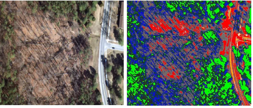
photography was chosen for this study because of its ability to capture the area of interest (PETE) at a large scale (1:6000) and at an affordable cost. True color and color infrared (CIR) photography were captured on March 13, 2004, mosaiced and orthorectified by SkyComp, Inc., of Columbia, MD, and delivered to North Carolina State University’s Center for Earth Observation in the summer of 2004. Upon initial visual inspection of the aerial photography, areas of downed woody debris were easily identifiable (Figure 3 and 4). However, manual delineation of the forest damage areas presented a lengthy and costly alternative. An automated approach to classifying the areas of downed woody debris was desired.
Traditional spectral analyses using both supervised and unsupervised
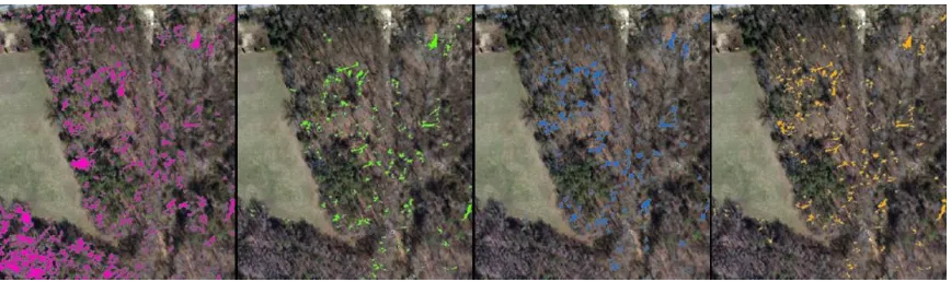
Upon visual inspection of the resulting classifications spectral confusion existed between areas of dead herbaceous matter (mowed grassfield) and areas of downed woody debris (Figure 3). A Normalized Differenced Vegetation Index (NDVI) classification of the image was performed, but the results were poor, as there was little green vegetation upon which the index could take place (Figure 4). It became apparent that spectral values alone could not be used to identify areas of downed woody debris. Traditional methods relying entirely upon spectral responses of pixels were inadequate for updating the existing fuel load and vegetation datasets. With areas of forest damage clearly
represented by downed trees, a classification technique that could map specific features is much better suited for fire potential (threat) research.
Figure 4: NDVI classification, outlines of some downed trees can be seen in blue.
5.1.2 Parameters of Feature Analyst
The following sections will outline the user defined parameters enabling Feature Analyst to classify an image based on spatial patterns. A detailed methodology of how the downed woody debris of the Fort Gregg area was classified is found in section 5.1.3. A similar procedure was followed to map other areas of PETE that had forest damage.
5.1.2a Training Sites
Figure 5 Example of training sites (in red) used to "train" Feature Analyst.
5.1.2b Pattern Recognizers and Initial Classification Attempts
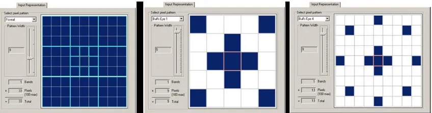
In addition to identifying the objects of interest, Feature Analyst must also be instructed on how to look for these objects. The software includes various pattern recognizers that examine each pixel to determine if it is in the target feature you are looking for. Nine types of pattern recognizers exist: Bull’s Eye 1, Bull’s Eye 2, Bull’s Eye 3, Bull’s Eye 4, Square, Circle, Manhattan, User Defined and Foveal. Some pattern recognizers indicate linear objects better, while others are better suited to indicate different types of land cover.
search window (Figure 6). This mimics a human’s peripheral viewing pattern; where the object of interest is in the center of view being focused on, while the outer areas are focused on less (Feature Analyst User’s Manual Version 4.0). The “best” classification was determined by visual inspection of the resulting classification.
Figure 6: VLS Feature Analyst's Pattern Recognizers Foveal, Bulls Eye 1 and Bulls Eye 4 used for delineating downed woody debris.
Figure 7: Classification results (left to right: Foveal, Bulls Eye 2 and Bulls Eye 1) for one iteration using different pattern recognizers.
Figure 8: Classification results (left to right: Iteration 1, 2, and 3) of the three iterations needed to map downed woody debris.
Feature selector allows the specification of the type of feature to be extracted from the imagery. Choices include; narrow linear feature, wide linear feature, natural feature, small manmade feature, manmade feature, landcover feature, water body feature, and building. The spatial resolution of the imagery being used is also entered.
The image’s bands to be analyzed are entered next. How each band is interpreted by Feature Analyst is determined as well, as the user can choose between; reflectance, texture, discrete, and elevation. Individual bands can be entered more than once and interpreted differently. For this research, texture was chosen as the method of interpretation for all iterations.
Parameters defining the learning file were chosen next; Approach 1, or general purpose, was chosen for all iterations. In initial classification attempts, Approach 1 provided the better classification results when visually compared to the other choices (Approach 2 and Approach 3). Another choice in this section was the aggregate area. The initial iteration was set at 50 pixels and reduced to 35 in subsequent iterations to further focus the classification results. The default settings of the Bezier smoothing algorithm were used when choosing the Smooth Polygons option. Lastly, the option to look for rotated features was selected.
5.1.2d True Color versus Color Infrared
Initial efforts focused on determining which image type was better suited for mapping downed woody debris. Using the True Color image, training sites were
types of imagery. The same training site polygon was used for all passes. After visual inspection of both classification results, the True Color image consistently provided a more accurate classification of downed woody debris when compared to the CIR
classification, and was chosen as the type of imagery to use for mapping downed woody debris at PETE.
5.1.3 Mapping Downed Woody Debris
The following section describes the steps taken to successfully classify downed woody debris of the Fort Gregg area of PETE. This same general methodology was used on additional sections of PETE as covered in section 5.1.4.
A training site polygon consisting of six occurrences of downed woody debris representative of the forest damage was created. For example, one site represented a single tree and its rootball, with other sites consisting of multiple trees and varying amounts of crown damage. Each polygon digitized consisted of at least 20 pixels.
The first pass utilized the following parameters, feature selector set to small linear feature, followed by learning settings set to all available bands and textures. Next under the input representation tab, the pattern recognizer, Fovel was chosen with a pattern width of 100. Finally, under the Learning Settings tab, Approach 1 with a minimum area of 50 pixels set and the find rotated instances option chosen.
pattern width of 75 chosen. Finally, under the Learning Settings tab, Approach 1 with a minimum area of 50 pixels set and the find rotated instances option chosen.
The third pass utilized the following parameters, feature selector set to small linear feature, followed by learning settings set to all available bands and textures. Next under the input representation tab, the pattern recognizer, Bull’s Eye 4 was chosen with a pattern width of 35 chosen. Finally, under the Learning Settings tab, Approach 1 with a minimum area of 50 pixels set and the find rotated instances option chosen.
The fourth pass utilized the following parameters, feature selector set to small linear feature, followed by learning settings set to all available bands and textures. Next, under the input representation tab, the pattern recognizer, Circle was chosen with a pattern width of 60 chosen. Finally, under the Learning Settings tab, Approach 1 with a
minimum area of 50 pixels set and the find rotated instances option chosen.
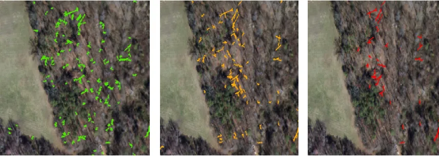
Figure 9: Example of four passes of the first iteration. After visual inspection the “best” classification is chosen for the second iteration.
With areas indicated as correct and incorrect the second iteration could begin. This time Feature Analyst analyzed only areas previously classified, and used areas identified as correct and incorrect to further focus its classification. The second iteration first pass utilized the following parameters, feature selector set to small linear feature, followed by learning settings set to all available bands and textures. Next under the input representation tab, the pattern recognizer, Foveal was chosen with a pattern width of 100. Finally, under the Learning Settings tab, Approach 1 with a minimum area of 50 pixels was set.
chosen with a pattern width of 35 chosen. Finally, under the Learning Settings tab, Approach 1 with a minimum area of 50 pixels was set.
The second iteration fourth pass utilized the following parameters, feature selector set to small linear feature, followed by learning settings set to all available bands and textures. Next under the input representation tab, the pattern recognizer, Bull’s Eye 3 was chosen with a pattern width of 35 chosen. Finally, under the Learning Settings tab, Approach 1 with a minimum area of 50 pixels was set.
Again the “best” classification of the second iteration was chosen based on visual interpretation of the image. Clutter removal was done next on the classification with areas identified as correct and incorrect. The more sites identified as correct or incorrect actually confuses the pattern recognizer in the next iteration of classifications, so it is recommended to limit areas identified to no more than 20.
The third iteration first pass utilized the following parameters, feature selector set to small linear feature, followed by learning settings set to all available bands and texture. Next under the input representation tab, the pattern recognizer, Bulls Eye 3 was chosen with a pattern width of 35 chosen. Finally, under the Learning Settings tab, Approach 1 with a minimum area of 35 pixels was set.
The third iteration third pass utilized the following parameters, feature selector set to small linear feature, followed by learning settings set to all available bands and
textures. Next under the input representation tab, the pattern recognizer, Manhattan was chosen with a pattern width of 27 chosen. Finally, under the Learning Settings tab, Approach 1 with a minimum area of 35 pixels was set.
The third iteration fourth pass utilized the following parameters, feature selector set to small linear feature, followed by learning settings set to all available bands and textures. Next under the input representation tab, the pattern recognizer, Bull’s Eye 1 was chosen with a pattern width of 35 chosen. Finally, under the Learning Settings tab, Approach 1 with a minimum area of 35 pixels was set.
The “best” classification of the third iteration was chosen based on visual
interpretation of the image and classification shapefile. Clutter removal was done again on the classification. However, on subsequent passes, the resulting classifications were actually less accurate as areas that clearly represented downed woody debris were excluded. As a result, The Bull’s Eye 1 third iteration classification was chosen as the “best”. Additional manual edits were done to remove polygons from the classification that were clearly not downed woody debris but closely resembled the spatial pattern of it (e.g. tree shadow on grassfield).
5.1.4 Additional Sections of Petersburg National Battlefield
In addition to the Fort Gregg area, the Fort Wadsworth and Fort Fisher sections of the Western Front also suffered damage as a result of Hurricane Isabel. To map these areas, a polygon training site shapefile consisting of ten occurrences of both deciduous and coniferous downed woody debris was created. Using the Foveal pattern recognizer for the initial iteration, those portions of the Western Front that were definitely not downed woody debris (e.g. cars, homes, homogenous stands of trees, mowed grasslands) were eliminated from further analyses. These areas were removed from future analyses because their spatial and spectral patterns did not resemble those of the training sites. Based on visual inspection, the Bull’s Eye 4 pattern recognizer was chosen as the “best” output classification for the second iteration. However, the resulting classification required the manual addition of several areas of downed woody debris as areas of coniferous species were not accurately indicated. The presence of both deciduous and coniferous trees in the training site shapefile probably led to this classification problem, as this did not occur in the Fort Gregg section.
addition to manually adding areas of downed woody debris, several examples of “correct” and “incorrect” areas of downed woody debris were identified in the “best” classification. The downed woody debris of the Fort Wadsworth and Fort Fisher areas of the Western Front of PETE was accurately classified after six iterations.
The Eastern Front section of PETE is the largest contiguous part of the park and suffered the most damage as a result of Hurricane Isabel. With deciduous, coniferous, and mixed forests present, two sets of training sites were necessary to represent the downed woody debris present. (Coniferous trees are small in size and typically black in color while deciduous trees are larger and either white or brown in color). The deciduous downed woody debris training site consisted of ten polygons, while the coniferous
training site consisted of seven polygons. Two separate training site shapefiles representing the different origin of species of the downed woody debris focused the Feature Analyst classification; ultimately reducing the number of iterations needed to achieve an acceptable classification.
Once accurate automated classifications for all affected areas of PETE were reached, the results were merged into one shapefile. This shapefile was then manually edited by visual inspection to further remove those features classified as downed woody debris. Confusion still existed in areas where shadows of tree branches or the tree branches themselves overlaid homogenous areas; creating a spatial pattern similar to downed woody debris. This manual edit reduced the number of downed woody debris polygons from 14,256 to 7,726.
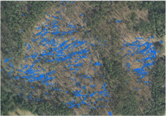
Figure 10: Example of mapped downed woody debris of the Eastern Front portion of PETE.
5.1.5 Construction of Forest Damage Polygons
smaller fuels like 1-, 10-, and 100-hour were not indicated. To capture these fuels, a generalized buffer, or forest damage polygon, was created around the mapped downed woody debris. (Examples of forest damage are uprooted tree pits and mounds and tree crowns snapped and lying on the ground, as shown in Figure 11). Applying the default settings of the Bezier smoothing algorithm (within Feature Analyst), downed woody debris represented as polygons, were converted to lines. The resulting downed woody debris line shapefile was used in ESRI’s ArcToolbox’s line density tool to create the generalized forest damage polygon. The output parameters, cell size and search radius, were set at one and five respectively. Cell size determined the resolution of the output grid, with each pixel measuring one meter. The search radius parameter, similar to a filter, set the size of the window that was used to calculate the cell values (0.0 to 1.0) of the resulting line density grid.
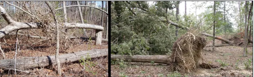
Figure 11: Examples of downed woody debris not detached from its point of origin.
shapefile that consisted of 2,891 polygons ranging in size from .0283 to 42,127 square meters. The “eliminate” tool in ArcToolbox 9.0 was used to dissolve smaller polygons, those less than 90 square meters, into the larger surrounding polygon. The final forest damage polygon consisted of 2,368 polygons, ranging in size from 2,104 to 102,139 square meters (.002 acres to 25.2 acres) (Figure 12).
The generalization of downed woody debris captured 1-, 10-, and 100-hour fuels missed by Feature Analyst classifications and captured the horizontal spatial continuum of downed woody debris across the landscape. With a minimum mapping unit of ½ an acre, only those forest damage polygons greater than ½ acre were considered for further study (51 in total). The majority of the polygons removed from consideration represented single occurrences of downed woody debris. Single downed trees do not represent an increase in fuel loading and therefore do not warrant updating the existing fuel model spatial dataset. Of the remaining 51 forest damage polygons the acreages ranged from 0.52 to 25.2 acres.