ABSTRACT
DAVE, GAURAV. Progressive Damage Analysis of Composite laminates under Fatigue: A Step-Based Method. (Under the direction of Dr. Mark Pankow).
Progressive Damage Analysis of Composite laminates under Fatigue: A Step-Based Method
by Gaurav Dave
A thesis submitted to the Graduate Faculty of North Carolina State University
in partial fulfillment of the requirements for the degree of
Master of Science
Mechanical Engineering
Raleigh, North Carolina 2017
APPROVED BY:
_______________________________ _______________________________
Dr. Scott Ferguson Dr. John Strenkowski
DEDICATION
BIOGRAPHY
Gaurav Dave was born and raised across various towns and cities of India. He pursued a Bachelor’s degree in Mechanical Engineering at Rashtraeeya Vidyalaya College of Engineering (Visvesvaraya Technological University). After graduating in 2013, he decided to join the workforce and gain valuable technical experience. He joined Tata Technologies as a Design Engineer. Here, he was involved in the body design for automotive clients.
In 2015, he started his Master’s program in Mechanical Engineering at North Carolina State University. At NC State, he was a part of the BLAST Lab under Dr. Mark Pankow, where he pursued his research interests in composite materials, finite element analysis, and additive manufacturing.
ACKNOWLEDGMENTS
First and foremost, I would like to thank Dr. Mark Pankow for his constant guidance and support over the past two years. Right from giving me an opportunity to work with him, to solving my copious, sometimes trivial doubts, and to ensure my research didn’t side-track, I don’t think I would have found a better mentor than him.
I would also like to extend my heartfelt gratitude to Dr. Scott Ferguson and Dr. John Strenkowski for serving on my committee. The courses I took under them played a vital role in my development as a graduate student.
I am also glad to thank all my fellow mates at the BLAST Lab for truly making research so much more fun in the lab. A special shout out to Shreyas, for always being the go-to guy for any doubts related to modeling, and teaching me some truly time-saving modeling techniques. And to Raghav, for being the perfect research partner. There were numerous instances that his optimism and humor were the only things that kept me going.
I was lucky to have landed a great group of friends at NC State, be it my flat mates, or my extended study circle. Thank you all for bearing with my incessant and unnecessary rants, and always being there for me.
TABLE OF CONTENTS
LIST OF TABLES ... viii
LIST OF FIGURES ... ix
1. INTRODUCTION ... 1
1.1 Fatigue Failure mechanisms in composites ... 1
1.2 Fatigue damage modeling in composites: Motivation ... 3
1.3 Historical background ... 4
1.4 Recent developments... 6
1.5 Research Objectives ... 9
1.6 Thesis Outline ... 12
2. FATIGUE DAMAGE MODELING ... 13
2.1 Damage initiation ... 14
2.1.1 In-plane ... 14
2.1.2 Interlaminar ... 15
2.2 Damage evolution ... 16
2.3 Input properties for the model ... 19
2.3.1 In-plane shear strength ... 19
2.3.2 Tensile Longitudinal Fracture energy ... 19
2.3.3 Peak tractions ... 20
2.4 Fatigue degradation ... 20
2.5 Step wise approach ... 24
3. FEA IMPLEMENTATION AND PRELIMINARY STUDIES ... 30
3.1 User subroutines ... 30
3.2 Element formulations used ... 33
3.2.1 Conventional shell element S4R ... 33
3.2.2 Continuum shell element SC8R ... 34
3.3 Single element studies ... 35
3.3.1 Degradation only in the fiber direction ... 36
3.3.2 Degradation only in the matrix direction ... 37
3.3.3 Degradation only in in-plane shear ... 38
3.3.5 Combined degradation in the fiber direction and the cohesive zone ... 42
3.3.6 Conclusion ... 44
4. CHALLENGE PROBLEM: S4R ELEMENT ... 45
4.1 Scope of present work ... 45
4.2 AbaqusTM Model Preparation ... 45
4.2.1 Geometry... 45
4.2.2 Argument against quarter symmetry model ... 46
4.2.3 Loading conditions... 47
4.2.4 Measurement of stress and strain ... 48
4.3 Mesh sensitivity... 48
4.4 Results and Discussion for [0/45/90-45]2s laminate with S4R elements ... 51
4.4.1 Damage after 300K cycles ... 51
4.4.2 Residual stiffness and strength... 54
4.4.3 Preliminary Conclusion ... 56
4.5 Effect of Binning Strategy... 57
4.6 Results and Discussion for [60/0/-60]3s laminate with S4R elements ... 60
4.6.1 Damage after 200K cycles ... 61
4.7 Overall Observations ... 62
5. CHALLENGE PROBLEM: SC8R ELEMENT ... 63
5.1 Modeling considerations for computational efficiency ... 63
5.1.1 Cohesive zone approximation ... 63
5.1.2 Contact formulation ... 64
5.2 Results and Discussion for [0/45/90/-45]2s laminate with SC8R elements ... 65
5.2.1 Only in-plane fatigue degradation ... 65
5.2.2 In-plane and Cohesive degradation ... 74
5.2.3 Overall takeaways for [0/45/90/-45]2s laminate ... 78
5.3 Blind Prediction for [60/0/-60]3s laminate with SC8R elements ... 79
5.3.1 Damage after 200K cycles ... 80
5.3.2 Residual stiffness and strength... 81
5.3.3 Overall takeaways for [60/0/-60]3s laminate ... 82
6. CONCLUSIONS AND FUTURE WORK ... 83
6.2 Future Work ... 85
LIST OF TABLES
Table 1.1 Blind results of PDA techniques versus experimental data [21] ... 11
Table 1.2 Recalibrated results of PDA techniques versus experimental data [21] ... 11
Table 2.1 Relevant static properties of IM7/977-3 lamina [12] ... 21
Table 2.2 Summary of fatigue degradation laws ... 23
Table 2.3 Binning strategies for step wise fatigue model ... 24
Table 2.4 Degraded properties implemented in FEA ... 29
Table 4.1 Mesh sensitivity study ... 49
LIST OF FIGURES
Figure 1.1 Common Failure mechanisms in a composite laminate [3] ... 2
Figure 1.2 Damage progression with life [4] ... 3
Figure 2.1 Principal directions for a unidirectional lamina ... 16
Figure 2.2 Stress displacement relation for in-plane damage evolution ... 17
Figure 2.3 Linear damage evolution for cohesive zones ... 18
Figure 2.4 Transition from static to degraded properties in 1-direction for an element ... 23
Figure 2.5 Degradation of longitudinal tensile strength under fatigue ... 25
Figure 2.6 Degradation of transverse tensile strength under fatigue ... 26
Figure 2.7 Degradation of in-plane shear strength under fatigue ... 26
Figure 2.8 Degradation of Tensile Longitudinal Fracture Energy under fatigue ... 27
Figure 2.9 Degradation of Tensile Transverse Fracture Energy under fatigue ... 27
Figure 2.10 Degradation of Mode II Fracture Energy under fatigue ... 28
Figure 2.11 Degradation of Peak shear traction under fatigue ... 28
Figure 3.1 Loading Profile and Field Variable in Bin1 ... 32
Figure 3.2 Loading Profile and Field Variable in Bin2 ... 32
Figure 3.3 Schematic of the S4R shell element ... 34
Figure 3.4 Schematic of the SC8R continuum shell element ... 35
Figure 3.5 Boundary conditions for single element cases ... 36
Figure 3.6 Fiber failure initiation and fiber damage evolution ... 37
Figure 3.7 Matrix failure initiation and matrix damage evolution... 38
Figure 3.8 Matrix failure initiation and shear damage evolution ... 39
Figure 3.9 Top view of boundary conditions for only Mode II cohesive degradation ... 40
Figure 3.10 Cohesive failure initiation and damage evolution ... 41
Figure 3.11 Traction separation response with fatigue degradation ... 41
Figure 3.12 Top view of boundary conditions for Mode II cohesive and fiber degradation .. 42
Figure 3.13 Cohesive damage initiation and evolution for combined degradation ... 43
Figure 3.14 Hashin fiber failure criterion for combined degradation ... 43
Figure 3.15 Traction separation with fatigue for combined cohesive and fiber degradation . 44 Figure 4.1 Open-hole Geometry used in experiments [35] ... 46
Figure 4.2 Open-hole FE Geometry without gripping regions ... 46
Figure 4.3 Representation of the pitfalls in a quarter symmetry for composites using a 45° ply ... 47
Figure 4.4 Mesh sensitivity results ... 50
Figure 4.5 Fiber damage (DAMAGEFT) in 0° layer after load-drop across meshes ... 50
Figure 4.6 Matrix in-plane damage (DAMAGEMT) versus experimental X-Ray CT images [12] ... 53
Figure 4.7 Residual static tension response: S4R vs Experiment ... 55
Figure 4.8 Comparison of Local and Global strains in the FE model ... 56
Figure 4.10 Matrix in-plane damage (DAMAGEMT) comparison using different binning
strategies ... 59
Figure 4.11 Residual stress strain response compared for Bin1 and Bin2... 60
Figure 4.12 Matrix in-plane damage (DAMAGEMT) versus experimental X-Ray CT images [12] ... 61
Figure 5.1 Cohesive zone approximation on each surface ... 64
Figure 5.2 Matrix in-plane damage (DAMAGEMT) and Delamination damage (CSDMG) versus experimental X-Ray CT images [12] ... 67
Figure 5.3 Matrix in-plane damage (DAMAGEMT) versus experimental X-Ray CT images [12] at center of the laminate ... 68
Figure 5.4 Residual static tension response for only in-plane fatigue degradation ... 72
Figure 5.5 Comparison of residual stress strain curves from PDAs [21] ... 72
Figure 5.6 Inertial and hourglassing effects in an implicit dynamic analysis ... 73
Figure 5.7 Matrix in-plane damage (DAMAGEMT) and Delamination damage (CSDMG) versus experimental X-Ray CT images [12] ... 75
Figure 5.8 Comparison between only in-plane degradation and combined degradation ... 76
Figure 5.9 Residual static tension response for both cohesive and in-plane fatigue degradation ... 77
Figure 5.10 Fiber in-plane damage (DAMAGEFT), matrix in-plane damage (DAMAGEMT), and Delamination damage (CSDMG) versus experimental X-Ray CT images [12] ... 80
1.INTRODUCTION
Fiber reinforced composites have come a long way today and are proving to be efficient in several lightweight structural applications which span across a diverse group of industries including the aerospace, automotive, energy and construction sectors. For any service part designed for these industries, failure due to fatigue is a necessary, often mandatory design parameter, and this hold true for composites as well. During their initial years, composites were touted to perform a lot better under fatigue when compared to metals [1]. In fact, this is true if the composites are loaded in the fiber direction, where there is little to no difference between the static and fatigue strengths [2]. However, with greater use of these materials in complex parts under various loading configurations, it would be wrong to adjudge that composites are unaffected by the number of service cycles.
1.1 Fatigue Failure mechanisms in composites
To understand fatigue in fiber reinforced composites, it is important to recognize the difference in the failure mechanisms involved in metals and composites. In metals, dislocation movements in the crystal structure are the primary cause of microscopic cracks, which then coalesce to form a large macroscopic crack leading to final failure. On the other hand, fiber reinforced composites, being heterogeneous in nature, can undergo multiple failure mechanisms during their course of loading. These mechanisms, in various combinations, govern a majority of loading cases, including static and fatigue loading. This distinguishes the behavior of composites from metals exhibiting isotropy under fatigue.
microbuckling, and delamination. A schematic diagram to distinguish between the common failure mechanisms is shown in Figure 1.1.
Figure 1.1 Common Failure mechanisms in a composite laminate [3]
Figure 1.2 Damage progression with life [4]
1.2 Fatigue damage modeling in composites: Motivation
The challenges mainly lie in modeling the varying scale of the damage and the different mechanisms discussed above. Despite this, there are inherent advantages of modeling damage for fatigue. An experimental testing exercise for fatigue loading is difficult, expensive, and time consuming. Also, if the progression has to be monitored, expensive non-destructive techniques have to be employed. A working damage model implemented with FEA reduces the overall time to bringing a component to production. It also provides with a predictive indication to how changing properties would affect the part’s performance. In the aerospace industry in particular, the regulations also require a working model along with experimental testing for composite parts. This serves as ample motivation to develop progressive damage models for composites which can predict the part’s fatigue performance.
1.3 Historical background
Since the 1970s, a large number of researchers in the field of composite materials have concentrated on understanding and modeling fatigue failure in fiber reinforced composites. An extensive review of various fatigue life models was carried out by Degrieck and Van Paepegem in 2001 [5]. The different fatigue models were classified into 3 categories as: 1) Fatigue life based models, 2) Phenomenological models based on Residual Strength/Stiffness, and 3) Progressive damage models based on mechanisms of damage.
constant-life model. A bell shaped fatigue function was defined in this model to fit the experimental data on a traditional Goodman type diagram. Bell shaped functions were used as they were better fits to composite data than the linear or parabolic fits previously used for metals. Harris and his coworkers were able to generate such curves for different stress values and stress ratios for glass reinforced and carbon reinforced laminates. Along similar lines, other life based models are discussed in the review paper by Degrieck and Van Paepegem. A common observation in these class of models is their simplistic nature in predicting only fatigue life, and their inability to track the course of actual damage in the composite specimen. Another drawback is that most of them require a large set of S-N data for each laminate sequence and material system.
The third class of models, called Progressive damage analysis (PDA) by a number of researchers, describe the deterioration of the composite material with respect to the actual damage in the specimen, be it matrix cracks, delamination size, or any other type of damage. As actual damage is modeled here, these techniques allow for modeling on different size scales, from micro level to macro level. This variation is possible as these techniques generally exploit the principles of fracture mechanics and thermodynamics, either separately or in combination, to model the actual damage in the specimen. A brief overview is outlined, followed by the recent developments in PDAs for fatigue modeling.
A fracture mechanics approach based PDA would model the crack initiation and propagation, and predict the density and location of the damage using material properties like the strain energy release rate, and geometrically dependent properties like the crack length. The direction of the crack would be decided based on the fiber orientation, whereas crack growth would involve a power law relation akin to the Paris’ law for metals.
Another approach would correlate damage to mechanical property reduction: namely strength and stiffness. From initial closed form solutions using shear lag analysis, these approaches have now migrated toward defining damage variables based on thermodynamic principles [9] [10]. As can be seen in the next section, a lot of these micro-level damage models scale up to continuum damage at the ply level.
1.4 Recent developments
techniques under static and fatigue loading in tension and compression. The objective of this exercise was to improve durability and damage tolerance analysis of composite aircraft structures. Lamina level experiments were provided by AFRL and a blind prediction on the open-hole specimens was performed by the participants. Afterwards, they were given the experimental results and allowed to recalibrate their models. Further details of the program and its participants could be found in the benchmarking paper by Clay and Engelstad [11]. The results of the experimental section of the exercise were published by Clay and Knoth [12]. A total of 9 PDAs participated in the program, of which 7 could model fatigue at present.
One primary differentiator between these techniques is the scale for modeling in-plane damage. In some techniques ( [13] [14] [15]), the in-plane damage (matrix cracks, splitting, etc.) is modeled on the micro level, where the constituent fiber and matrix properties are used to evaluate the overall damage in the composite laminate. This puts them in the category of property reduction based on energy principles. In other techniques ( [16] [17] [18]), the in-plane damage is modeled on the ply level properties (macro-level damage). It is to be noted that MAC/GMC is a micromechanics based approach, but a macro level approach was used by its authors for this exercise. Micro level modeling could better predict the extent of damage, but their computational expense has to be minimized.
create a damage zone to show in-plane damage, albeit using the same principles. It is clear that a discrete crack technique better captures the physics when compared to a diffused damage zone, and this is validated by the X-Ray CT images from the experimental results by Clay and Knoth in [12]. However, there is a higher level of fidelity required when modeling a discrete model, either by modeling in-plane cohesive elements or aligning the mesh to match fiber orientations. Also, in a large number of such models, a manual crack insertion is required as in input for crack propagation using Paris’ Law. This partially invalidates the results from the analysis being truly "blind". It is believed that if a continuum damage approach can model all the failure mechanisms, it could be an efficient method for modeling damage.
computational cost of using cohesive elements. In this work, an attempt has been made to understand the effect of the degradation of delamination using cohesive zones under fatigue loading on the residual response of the laminate in question.
1.5 Research Objectives
Overall, the performance of these techniques in the exercise was reviewed by Engelstad and Clay [21]. Table 1.1 and Table 1.2 show the results when compared with experimental data before and after recalibration for tension-tension fatigue of a [0/45/90/45]2s quasi-isotropic laminate. The average error in recalibrated residual strength and stiffness was 13% and 4% from the experimental results, respectively. It was acknowledged by the authors that technology gaps exist in effectively modeling delamination in fatigue, either discreetly, or via reducing stiffness. Using this data, an opportunity presented itself wherein the effect of delamination could be studied on a macro level continuum damage model. A novel and simplified step-based method for damage progression was devised, and it was a relevant question to compare its performance to the state of the art PDAs. The above factors influenced the overall research objectives of this work, which are as follows:
1. To evaluate the performance of a step based method with macro-level continuum damage against the experimental data from AFRL and the state of the art PDA codes under tension-tension fatigue loading.
2. To study the effect of cohesive zone degradation on the overall damage and the computational cost for a sample laminate from the AFRL challenge problem.
method will be used as an approximation of the cycle-by-cycle degradation. This will then be implemented on 2 element formulations, with and without delamination modeling capabilities. Both sets of results will then be individually compared against the experimental data and other codes.
Table 1.1 Blind results of PDA techniques versus experimental data [21]
Blind Experiment MAC/GMC Helius
PFA MDS-C
BSAM-MIC DCN GENOA EHM
Average error %
Open-hole tension Residual strength
(MPa)
544 342 475 498 684 450 498 522 16
Residual stiffness after fatigue 300K
cycles (GPa)
47 48 32 48 40 50 52 48 10
Table 1.2 Recalibrated results of PDA techniques versus experimental data [21]
Recalibrated Experiment MAC/GMC Helius
PFA MDS-C
BSAM-MIC DCN GENOA EHM
Average error %
Open-hole tension Residual strength
(MPa)
544 436 552 613 601 462 403 523 13
Residual stiffness after 300K cycles
(GPa)
1.6 Thesis Outline
Chapter 2 covers the fundamentals of the continuum damage model used in this work and the step based fatigue damage approach based on the continuum model. The material properties used and required by the model, their justification in use, and their degradation under fatigue are also covered in this chapter.
Chapter 3 describes the transition from the theory of Chapter 2 to its implementation into a finite element analysis software. In order to prove the working of the model, single element studies were carried out, the details of which are also discussed in this chapter.
Chapter 4 defines the scope of the challenge problem to be tackled in this work. During the course of this research, 2 distinct element formulations were used. The first element formulation (S4R) is incapable of handling cohesive zone modeling. The results and discussion of the challenge problem with this formulation are covered in this chapter. Additionally, ‘blind’ results from the second stacking sequence with this element are also included.
Chapter 5 describes the specific modeling nuances associated with the second element formulation, which can model delamination. The results and discussion of the challenge problem with this formulation are covered. The effect of degrading cohesive properties in the challenge problem is also discussed. In the end, the ‘blind’ predictive results for the second laminate sequence and its implications conclude the chapter.
2.FATIGUE DAMAGE MODELING
This chapter discusses the theory behind the continuum damage model and the novel step-based method for fatigue modeling used in this work.
2.1 Damage initiation
2.1.1 In-plane
In-plane damage is governed by the criteria put forward by Hashin and Rotem [22] which separates fiber failure and matrix failure.
Case 1: Fiber tension (
11 0)
2 2
11 12
1
ft T L
F X S
(2.1)
Case 2: Fiber compression (
11 0) 2 11 1 fc C F X (2.2)
Case 3: Matrix tension (
22 0)
2 2
22 12
1
mt T L
F Y S (2.3)
Case 4: Matrix compression (
22 0)
2 2
2
22 22 12
1 1
2 2
C
mc T T C L
Y F
S S Y S
(2.4)
Here,
ij
YC are transverse (2 direction) tensile and compression strengths, and SL and ST are the longitudinal (1-2 plane) and transverse (2-3 plane) shear strengths, respectively. For reference, a typical unidirectional lamina and the principal axes are shown in Figure 2.1. The parameter
in Equation (2.1) allows for the effect of shear on the 1-direction tension in Hashin’s model. It ranges from 0 to 1, with an increase in the effect of shear from 0 to 1.
For the challenge problem, only the fiber and matrix tension cases are applicable due to the nature of loading. This means that the damage variables in fiber tension dft, matrix tension
mt
d , and in-plane shear ds, should be looked at during the analysis. The value of is chosen to be 1, which meets Hashin’s model [22].
2.1.2 Interlaminar
Damage initiation for cohesive zones is based on the peak tractions in the normal and shear directions. In the present work, the applied loading is in-plane loading; this would primarily lead to higher shear tractions. This is the reason for choosing a maximum nominal stress criterion for damage initiation and no mixed mode behavior as shown below. For a mixed mode loading scenario involving Mode I and Mode II interactions, the Benzeggagh-Kenane (B-K) parameter could be employed, for which the data is available.
0 0 0
max n , s , t 1 n s t t t t t t t
(2.5)
In Equation(2.5), the normal traction tn and out-of-plane shear traction tt are very small compared to ts for the loading case in question. Hence, cohesive damage is initiated simply when the in-plane shear traction reaches peak value, 0
2.2 Damage evolution
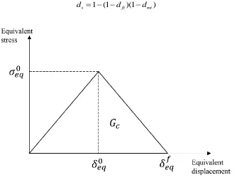
For in-plane damage, once the damage initiation criteria are met, damage variables increase from 0 to 1, and their evolution is decided by the translaminar fracture energy for that particular failure mode, the equivalent stress eq and equivalent displacement eqas per Equation(2.6).
0 0
( )
( )
f
eq eq eq f eq eq eq
d
(2.6)
Figure 2.1 Principal directions for a unidirectional lamina
linear damage evolution, and further details on their calculation can be found in the documentation for AbaqusTM [27].
Finally, based on the value of individual damage variables, the plane stress stiffness matrix of the element is modified as per Equation(2.7).
1 21 1
12 2 2
(1 ) (1 )(1 ) 0
1
(1 )(1 ) (1 ) 0
0 0 (1 )
f f m
d f m m
s
d E d d E
C d d E d E
D d GD (2.7)
Here, D 1 (1 df)(1dm) 12 21. As the present work deals only with tensile loading, the shear damage is simplified to:
1 (1 )(1 )
s ft mt
d d d (2.8)
Figure 2.2 Stress displacement relation for in-plane damage evolution
shear strengths. Thus, from Equation (2.8), the shear damage and the matrix damage are equal as per this model.
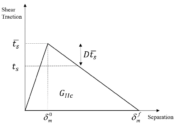
For cohesive zone damage evolution, a similar law is applicable, which is understandable as it is based on the traction-separation law first developed for cohesive element damage. A single scalar damage variable D is used and derived from the Mode II fracture energy GIIC, and it evolves over time in a manner similar to the in-plane damage variables from Equation(2.6).
Using this damage value and extrapolated elastic traction for the current straints, the damaged traction is given by:
(1 )
s s
t D t (2.9)
Figure 2.3 portrays a good idea of how a linear damage law for traction separation in pure shear would work.
2.3 Input properties for the model
One of the primary research objectives in this work was to use the high quality lamina level experimental data for fatigue from AFRL [12] and to predict the fatigue response of a composite laminate. In this regard, every effort was made to use the static material properties for IM7/977-3 graphite epoxy as provided by AFRL to all PDAs for the exercise. Any additional/modified input is duly noted by an asterisk in Table 2.1, and discussed herein.
2.3.1 In-plane shear strength
Due to the limitations of the Hashin model in AbaqusTM, implementing shear nonlinearity is difficult, therefore the in-plane shear strength is assumed to be linear, and derived from the tests on a [45/-45]4s laminate. From AFRL [12], the axial tensile strength of the [45/-45]4s laminate is found to be 220MPa. For a high-strength composite with E1>>E2, the in-plane shear strength can be approximated as half of the axial tensile strength [28], i.e. 110MPa. It is acknowledged that this value is higher than the 80-100MPa range suggested by AFRL for the challenge problem. Most of the other PDAs approximated this value to be around 100MPa ( [13] [16] [17]).
2.3.2 Tensile Longitudinal Fracture energy
2.3.3 Peak tractions
A major assumption is made on the peak tractions for initiation of delamination for both modes, which stems from the lack of an ASTM standard for their measurement, and was not provided by AFRL. These properties are matrix dominated, and little to no experimental data was found in the literature for the 977-3 matrix system used. For Mode I traction, a comparable result to experiments was obtained by Ranatunga and Clay [31] for 15 MPa. Whereas for Mode II traction, Joglekar et al [32] used a value of 30 MPa, and comparable results to experiments were reported. Although these values are used for this work, it is recognized that there is a significant experimental roadblock to be crossed for better characterization, and the approach is at a disadvantage compared to the other PDAs which don’t require these traction inputs.
2.4 Fatigue degradation
For the fatigue model, the curve fit data on the S-N curves for a unidirectional lamina was provided by AFRL, and this was used to set up the individual degradation laws. The following static properties were degraded with an increasing number of cycles:
1. In-plane strengths in fiber direction (XT), matrix direction (YT), and in-plane shear (SL) 2. In-plane fracture energies corresponding to damage in fiber (GXT) and matrix direction
(GYT)
In addition, the effect of degrading the following cohesive properties on the overall response of the laminate is studied:
1. Traction 0
Table 2.1 Relevant static properties of IM7/977-3 lamina [12]
In-plane properties Units Value
Longitudinal modulus in tension, E1 MPa 164000
Transverse modulus in tension, E2 MPa 8980
Major Poisson's ratio 0.32
In-plane Shear Modulus, G12 MPa 5010
Tensile longitudinal strength, XT MPa 2905
Tensile transverse strength, YT MPa 78.9
In-plane shear strength, SL MPa 110*
Tensile longitudinal fracture energy, GXT kJ/m2 91.6* [30] Tensile transverse fracture energy, GYT kJ/m2 0.256
Cohesive zone properties
Peak normal traction, 0 n
t (MPa) 15* [31]
Peak shear traction, 0 s
t (MPa) 30* [32]
Mode I fracture energy, GIC (kJ/m2) 0.256
Mode II fracture energy, GIIC (kJ/m2) 0.65
In Table 2.2, ‘y’ represents the property to be degraded, and ‘N’ represents the number of cycles. Some highlights of the fatigue degradation law are as follows:
1. The curve fit equations from AFRL’s data are modified such that N=1 corresponds to the static value of the property. This adjustment is acceptable as it did not drastically change the goodness of the fit.
2. For in-plane shear data, the S-N curve for [45/-45]4s was used and the data was transformed to represent a pure shear case. Only in this case, the static tensile shear strength was also derived from the fatigue data.
4. The tensile transverse fracture energy and the Mode I fracture energy from DCB tests are both matrix dominant properties; this is why the DCB degradation curve was used for degrading GYT.
5. For the longitudinal direction, no fatigue data is available for GXT. Due to its definition based on the lines of a linear traction separation law, it should be proportionally degraded with XT to keep the ultimate damaged strain unchanged. Figure 2.4 shows a schematic diagram of how this is achieved by degrading GXT proportionally to XT. 6. Peak shear traction 0
s
t is degraded proportionally to GIIC because only degrading the energy would not impact the damage initiation, and subsequent increase in damage won’t be captured.
Although there are a number of ways stiffness degradation can be performed based on the failure state of the lamina [33] [34], it was decided not to degrade any stiffness terms with number of cycles because:
1. Experimental data on stiffness degradation increases the number of experiments to be performed, and the model’s target was to only use inputs from AFRL’s study.
Table 2.2 Summary of fatigue degradation laws
Property Experimental data source Curve-fit equation
Longitudinal tensile strength,
XT (MPa) 0 degree S-N curve 0.0386 log 1
2905 y N
Transverse tensile strength, YT (MPa)
90 degree 3 point bend S-N
curve 78.9 0.080 log 1
y
N
In plane shear strength, SL (MPa)
[45/-45]4s laminate S-N
curve 110 0.086 log 1
y
N
Tensile longitudinal fracture energy, GXT (kJ/m2)
Proportional to XT
degradation NA
Tensile transverse fracture energy, GYT (kJ/m2)
Double Cantilever Beam (DCB) GImax-N curve
0.092
0.258
y N
Mode II fracture energy, GIIC (kJ/m2)
End Notched Flexure (ENF) GIImax-N curve
0.114
0.648
y N
Peak shear traction, 0
s
t (MPa)
Proportional to GIIC
degradation NA
Figure 2.4 Transition from static to degraded properties in 1-direction for an element
2.5 Step wise approach
From the above section, it is theoretically possible to derive individual strengths and energies after any number of cycles, and use that to predict a laminate’s response. However, it is a computational nightmare to implement 300K analyses, one for each cycle. Keeping this in mind, a simple approach was used which could satisfy the primary objectives of the challenge problem, namely:
1. Overall damage in the specimen after 300K cycles
2. Residual stiffness of the specimen in static tension post 300K cycles 3. Residual strength of the specimen in static tension post 300K cycles
In a step wise approach proposed herein, it is assumed that the properties don’t change for a fixed number of cycles, and are consequently dropped to a lower value, and so on, as a step function. This way, properties are “binned” into steps of time where they remain unchanged. The drop in value is derived from the fatigue law discussed above. A binning strategy with 3 steps was selected as a starting point for the present work. In this case, the value of the strength/energy would remain same between N=1 and N=1000, and would be equal to the static (N=1) value. Following this, a step drop in this property reduces its value corresponding to N=1000. It will now remain the same between N=1000 and N=100K, and so on.
Table 2.3 Binning strategies for step wise fatigue model
Strategy Number of loading cycles
Bin1 1-1000 1000-100K 100K-300K
A second binning strategy with 6 steps was also used for the case with only in-plane degradation. Both strategies are shown in Table 2.3.
For this study, the individual graphs for degraded strengths and energies are shown in Figure 2.5-Figure 2.11. These graphs include the original curve fit law, as well as the 2 binning strategies. Table 2.4 summarizes the values of the degraded properties in both binning strategies. The next chapter would discuss how this fatigue model is implemented in finite element analysis (FEA).
Figure 2.6 Degradation of transverse tensile strength under fatigue
Figure 2.8 Degradation of Tensile Longitudinal Fracture Energy under fatigue
Figure 2.10 Degradation of Mode II Fracture Energy under fatigue
Table 2.4 Degraded properties implemented in FEA
Range XT
(MPa) YT (MPa) SL (MPa) GXT
(kJ/m2)
GYT
(kJ/m2)
GIIC
(kJ/m2)
0 s
t
(MPa) Bin1
1-1000 2905.0 78.90 110.00 91.60 0.256 0.650 30.00 1000-100K 2568.6 59.96 81.42 80.99 0.136 0.295 13.65 100K-300K 2344.3 47.34 62.37 73.92 0.089 0.175 8.08
Bin2
3.FEA IMPLEMENTATION AND PRELIMINARY STUDIES
3.1 User subroutines
From the fatigue damage model described in the previous chapter, it is clear that the material properties in Table 2.4 have to be modified during the course of analysis. As mentioned earlier, the commercial FEA package AbaqusTM was used in this study, and using user subroutines is a straightforward approach to this problem. The choice of a subroutine depends on the complexity of the problem. Since none of the properties in question are material constants (stiffness or compliance terms), a material model using the highly involved UMAT subroutine was not deemed necessary. Instead, user subroutines USDFLD and UFIELD were used, which utilize user defined field variables as input flags for changing the mechanical properties.
Using USDFLD, it is possible to define a field variable at a material point as a function of either a material point quantity, or analysis time (Note: In AbaqusTM terminology, a material point is an element integration point [27]. Similarly, UFIELD allows a field variable to be defined based on a nodal property or analysis time. In this work, the total time is used as an input to assign values to the field variables. It is worth noting that the in-plane properties (strengths and energies) can be manipulated using USDFLD, since they are defined in the material model assigned to each material point. The cohesive zone properties (energy and traction) are nodal, and hence their manipulation necessitates the UFIELD subroutine.
overall load applied is scaled as per the analysis time specified. This is exploited to create a loading profile as well as defining field variables. A triangular waveform, as shown in Figure 3.1, shows how a fatigue loading-unloading cycle with R=0.1 is implemented for the Bin1
strategy. Here, R is the ratio of the minimum load to the maximum load applied min max
R
.
Each peak of the profile corresponds to a single field variable value, which corresponds to a bin. This value of the field variable is then used to trigger the corresponding set of material properties using the above mentioned subroutines. Similarly, Figure 3.2 shows the loading unloading pattern and the field variable assignment for the Bin2 strategy.
Figure 3.1 Loading Profile and Field Variable in Bin1
3.2 Element formulations used
For a thin composite laminate loaded in the 1-2 plane, the shell element library in AbaqusTM is used instead of solid elements. It is important to note that Hashin’s damage model in AbaqusTM is not compatible with solid elements. Two types of shell elements, conventional shell and continuum shell elements can be used to discretize a composite lamina, and a brief description of these elements follows.
3.2.1 Conventional shell element S4R
The conventional shell element S4R is a 4 node plane shell element. Each node allows both translational and rotational degrees of freedom, and hence there are a total of 6 degrees of freedom per node, as shown in Figure 3.3. The thickness of the lamina is defined as a section property, and in this work, 3 section points are used to obtain 3 results for elemental properties along the thickness direction. S4R is a reduced order shell element, i.e., there is a single integration point. Using a reduced order element instead of fully integrated elements increases computational efficiency, but can potentially have hourglassing issues. So, the associated mode energy has to be kept in check. But hourglassing is not as big a problem under in-plane loading as it is for bending scenarios. As S4R is effectively a 2D element, contact modeling, including cohesive zone modeling, is not possible with this element type.
Figure 3.3 Schematic of the S4R shell element
3.2.2 Continuum shell element SC8R
Continuum shell elements are better suited to model through the thickness properties of a composite layer due to the 3D geometry of the element. SC8R is a finite strain reduced order continuum shell element which consists of 8 nodes. Each node in an SC8R element only has 3 translational degrees of freedom, as shown in Figure 3.4. The thickness is hence modeled as the geometry of the element. In this case, a single stack of SC8R elements were used to model a lamina of 0.127mm from the experimental exercise [12]. The 3D geometry allows for stacking of elements in the thickness direction and enables the definition of two-sided contact (using cohesive zones in the present work) between elements. In this work, the reduced order is used with 3 integration points per element, which helps in obtaining 3 outputs through the thickness for each layer, if needed.
Figure 3.4 Schematic of the SC8R continuum shell element
3.3 Single element studies
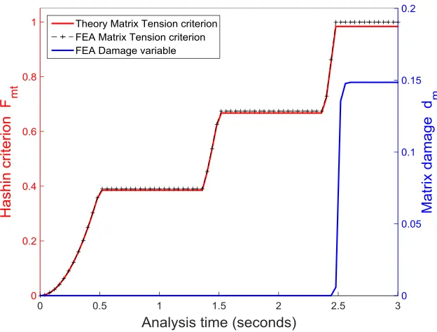
In order to benchmark the fatigue model described in Chapter 2, and to prove that it would perform as expected on the challenge problem, simple single element studies were conducted on the SC8R element, and the evolution of damage was matched with the theoretical formulation. A rectangular geometry (1mm x 1mm) with a layer thickness of 0.127mm [12] was loaded as per the profile in Figure 3.1 (Bin1 strategy). The magnitude of load applied was carefully chosen such that the effect of fatigue degradation could be observed. The following load cases were studied:
1. Degradation only in the fiber direction 2. Degradation only in the matrix direction 3. Degradation only through in-plane shear 4. Degradation of only the cohesive zone
Figure 3.5 Boundary conditions for single element cases
Left to Right: (a) Tension in 1 direction; (b) Tension in 2 direction; (c) Pure in-plane shear
3.3.1 Degradation only in the fiber direction
Figure 3.6 Fiber failure initiation and fiber damage evolution
3.3.2 Degradation only in the matrix direction
Figure 3.7 Matrix failure initiation and matrix damage evolution
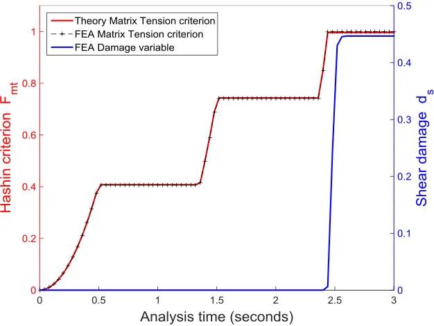
3.3.3 Degradation only in in-plane shear
modes are active, where the fiber is a lot stronger than the matrix. The comparison of Fmt between theory and FEA, as well as the evolution of dsis shown in Figure 3.8.
Figure 3.8 Matrix failure initiation and shear damage evolution
3.3.4 Degradation of only the cohesive zone
Unlike previous cases, degrading the cohesive zone under Mode II shear requires a 2 element model where one element is completely fixed while the other is moved, as shown in Figure 3.9. Only the shear traction in 1-2 plane is resisting this force to this type of loading. In the earlier cases, a USDFLD subroutine was used, whereas the UFIELD subroutine was used here for cohesive degradation. The peak traction 0
s
case, it can be calculated and matched with the FEA results, as shown in Figure 3.10, where the evolution of the cohesive damage variable D is also shown.
The effect of the degradation law in this case can be better visualized from the traction-separation behavior of the cohesive zone. This curve is shown in Figure 3.11. Once the peak value of 0
s
t is reached, an increase in D is prompted. This consequently decreases the stiffness in the 2nd loading cycle, where the degraded value of 0
s
t is used. As can be seen in Figure 3.11, displacement control was used instead of load control, as there are convergence difficulties associated with dropping stiffness under load control.
Figure 3.10 Cohesive failure initiation and damage evolution
3.3.5 Combined degradation in the fiber direction and the cohesive zone
The degradation of in-plane properties uses the USDFLD subroutine, and cohesive degradation is modeled by the UFIELD subroutine. In order to verify that their combination works as desired, a sample 2 element model was loaded such that both uniaxial tension in 1-direction and cohesive interaction in Mode II is present. The top view of the boundary conditions is shown in Figure 3.12. As the cohesive zone strength is of a smaller magnitude compared to the fiber strength, the cohesive damage initiation and evolution is captured easily, as shown in Figure 3.13. However, the Hashin fiber damage initiation criterion is very small, but increases in each step as expected, as seen in Figure 3.14. The traction-separation behavior is also slightly different than a pure cohesive degradation case due to the inherent stiffness of the element being pulled, as can be seen in Figure 3.15.
Figure 3.13 Cohesive damage initiation and evolution for combined degradation
Figure 3.15 Traction separation with fatigue for combined cohesive and fiber degradation
3.3.6 Conclusion
4.CHALLENGE PROBLEM: S4R ELEMENT
In this chapter, the overall scope of this work with respect to the AFRL exercise is outlined, followed by the nuances of general model preparation in AbaqusTM. A preliminary implementation of the step wise fatigue model using the plane shell formulation is also covered. The results are compared with experimental data and the advantages and limitations of using this formulation are discussed.
4.1 Scope of present work
As mentioned earlier, the AFRL round robin exercise and its experimental results form the basis for the problem solved in this work. AFRL’s experimental exercise was a two-step program, which consisted of a blind prediction phase followed by a recalibration phase based on experimental results. The experimental exercise was performed on 3 layup sequences: [0/45/90/-45]2s, [60/0/-60]3s, and [30/60/90/-60/-30]2s. The samples were loaded to a predefined number of cycles, followed by residual tension and compression tests. In order to get a preliminary idea whether the model proposed herein was on the right track, only the first laminate sequence ([0/45/90/-45]2s) was considered, with only a residual tension test post fatigue. In this chapter, the results of the plane shell formulation (S4R) for ([0/45/90/-45]2s are discussed. In addition, a blind prediction on the second laminate sequence ([60/0/-60]3s) and the challenges associated with that sequence is also discussed.
4.2 AbaqusTM Model Preparation
4.2.1 Geometry
modeled in the FE geometry, reducing the overall number of elements. An example of the FE geometry used is shown in Figure 4.2. Each layer, which is 0.127mm thick, is modeled based on the choice of elements. For the initial plane shell modeling using S4R elements, a 2D geometry is modeled with a composite layup where each layer is divided into 3 sections across the thickness of 0.127mm. For subsequent analyses with SC8R continuum shell elements (covered in the next chapter), each layer is represented by a 3D geometry 0.127mm thick, with 3 section points for through thickness variation.
Figure 4.1 Open-hole Geometry used in experiments [35]
Figure 4.2 Open-hole FE Geometry without gripping regions
4.2.2 Argument against quarter symmetry model
planar directions. This model is accurate for isotropic materials, but falls short when modeling a lamina with ply orientations other than 0º and 90º. For instance, the fiber orientation under quarter symmetry for a 45° ply is shown in Figure 4.3 on the left, whereas the actual ply orientation is displayed on the right. This necessitates the use of a full scale model in the present work.
Figure 4.3 Representation of the pitfalls in a quarter symmetry for composites using a 45° ply
4.2.3 Loading conditions
4.2.4 Measurement of stress and strain
To obtain the overall stress stain response from the FE model, the reaction force data in the loading direction was used to calculate the stress, and the nodal displacements in the loading direction at 2 centrally located nodes 25.4mm apart were used to calculate strain. Both of these regions are clearly marked in Figure 4.2. Assuming the tabs to be completely fixed by the grips, the total reaction force in the fixed nodes would be a good indicator of the load cell readout. Also, as the local strains near the hole are affected by its presence, measuring strain from central nodes will capture the local effects better when compared to far field strain measurement.
4.3 Mesh sensitivity
Table 4.1 Mesh sensitivity study
Reference Name
Total number of elements
Elements in Near-hole region
Peak Stress (MPa)
Coarse4 76 16 490.03
Coarse3 140 64 595.15
Coarse2 480 256 596.16
Coarse 868 576 572.78
Fine1 1296 784 585.25
Fine2 1796 1024 602.20
Fine3 2088 1296 589.00
Fine4 2416 1600 581.57
Figure 4.4 Mesh sensitivity results
Figure 4.5 Fiber damage (DAMAGEFT) in 0° layer after load-drop across meshes
the experimental value was deemed suitable for carrying out fatigue loading. It is important to note that the number of elements would compound for each layer when using the SC8R elements in the next chapter.
4.4 Results and Discussion for [0/45/90-45]2s laminate with S4R elements
4.4.1 Damage after 300K cycles
As mentioned earlier, only in-plane damage can be captured if plane shell S4R elements are used. The extent of the damage in the present model 300K cycles was compared to the X-Ray CT imaging data available from AFRL [12]. The overall contours for matrix damage variable dm and their comparison to experimental data is shown in Figure 4.6, where the loading direction is vertical. For the laminate [0/45/90/-45]2s in question, a repeating sequence results in identical FEA output, and hence the data shown is only from the first set of layers. It is well understood that longitudinal matrix cracks, which correspond to in-plane damage, are visible as straight lines on the X-Ray, whereas a light-colored area indicates delamination. Shear damage contours are identical to matrix damage contours due to how the Hashin model is set up, and either of them can be used to observe the evolution of matrix cracking.
Figure 4.6 Matrix in-plane damage (DAMAGEMT) versus experimental X-Ray CT images [12] Layer Matrix damage contour X-Ray CT images Interface Legend
45/90
90/-45
-45/0 0
45
90
-45
0
4.4.2 Residual stiffness and strength
Residual stiffness
The stress-strain response for the static residual tension test after 300K cycles are compared with the experimental data and shown in Figure 4.7. The experimental results in [12] are traced and plotted for a better comparison. The error in the residual stiffness between the experiments and the FE model is 8.9% (47GPa from experiments, 51.2GPa from the FE model). As the other theories also have an average error of 4% for this sequence, this is an acceptable value for a plane shell model.
Residual strength
The residual strength of the laminate is a relatively difficult value to arrive at using an implicit finite element analysis, due to the nature of the final failure. A quasi isotropic laminate like the one in question would finally fail resulting in two parts via fiber breakage. As the fibers have little to no plastic deformation, a sudden load drop would occur, as seen in Figure 4.8. In a finite element model with damage, this corresponds to a large number of 0° elements damaging in the fiber direction simultaneously, which makes it difficult for solution convergence. These effects are more influential in a 3D analysis, and possible solutions are discussed in the next chapter.
Figure 4.7 Residual static tension response: S4R vs Experiment
Overall response
Figure 4.8 Comparison of Local and Global strains in the FE model
Another aspect of the kink in the curve is the local strain relaxation near the holes. From Figure 4.8, a clear distinction is observed between strain calculated locally near the holes, and global strain calculated from overall applied displacement. In the area of interest, when the +/-45° plies are failing, the laminate is unable to take up any load and the global strain increases without any appreciable increase in stress (red in Figure 4.8). However, the local elements near the hole on the 0° piles experience some relaxation, since the load is not carried by them momentarily, which reduces the local strain (blue in Figure 4.8). Once all the intermediate plies have failed, only the 0º plies are carrying all the subsequent load until 2-part failure.
4.4.3 Preliminary Conclusion
capturing the damage progression (for instance, after 50K cycles). This drawback is addressed by using a 5 bin strategy in the next section.
4.5 Effect of Binning Strategy
Figure 4.9 Hashin Matrix initiation criterion (HSNMTCRT) comparison using different binning strategies
Bin1
Legend Bin2
Cycle Range 1000-100K 100K-300K
Figure 4.10 Matrix in-plane damage (DAMAGEMT) comparison using different binning strategies
Legend
1000-100K 100K-300K
Cycle Range
Cycle Range
Bin1 Bin2
Figure 4.11 Residual stress strain response compared for Bin1 and Bin2
For a 2D analysis, the difference in computational time is not noticeable between Bin1 and Bin2 (60 seconds to 90 seconds), but it is still 1.5 times computationally more expensive to run a Bin2 strategy, due to the sheer number of increments. This factor becomes significant when the run-time per iteration increases, as is the case of the 3D model. As the damage contours after 300K cycles and the residual strength and stiffness were the primary objectives when comparing with the AFRL data, the Bin1 strategy is employed moving forward, since these results remain unchanged between strategies.
4.6 Results and Discussion for [60/0/-60]3s laminate with S4R elements
4.6.1 Damage after 200K cycles
Due to the high percent of static load (80%) being applied in the fatigue loading, the fatigue property degradation of the present model led to 2 part failure in the laminate under fatigue loading. This does not match the experimental data, but the same problem was faced by 4 of the PDA codes as well in their blind predictions.
Figure 4.12 shows the comparison between a typical X-Ray CT image from experimental data and matrix damage in a 60° layer of the FE model. The matrix cracks in the 60° and -60°are captured quite well as failed regions in this work. The continuum nature of the model equally affects both the diagonal regions, not distinguishing between a 60° crack and a -60° crack. However, for this sequence, the failure mechanisms which are observed in experiments to be dominant are 0° fiber splits and delamination. It has already been discussed that this model is incapable of modeling fiber splitting. Also, as delamination cannot be predicted by S4R elements, this model fails in predicting the damage accurately for this laminate sequence.
Figure 4.12 Matrix in-plane damage (DAMAGEMT) versus experimental X-Ray CT images [12]
Legend Matrix damage contour X-Ray CT images
4.7 Overall Observations
1. For the laminate sequence of primary concern [0/45/90-45]2s, the in-plane matrix damage progression is predicted fairly by the model using a 3 bin strategy, which can be improved by increasing the number of bins.
2. The residual strength and stiffness prediction for the [0/45/90-45]2s sequence is also predicted close enough to the experimental results and other PDAs, with the overall error being under 10%. Hence, this model with a plane shell formulation offers a quick and fairly accurate idea on the in-plane damage and residual properties, and is extremely efficient computationally.
3. The inability of the plane shell model to capture delamination failure is a major drawback, which is highlighted in both the laminate sequences. This could be overcome by using a 3D FE model with SC8R elements in the next chapter.
5.CHALLENGE PROBLEM: SC8R ELEMENT
In this chapter, the challenge problem is solved using the SC8R element in AbaqusTM. The specific modeling considerations are discussed, followed by results and discussion of the laminate in question ([0/45/90/-45]2s). This is then followed by blind prediction results using this element for the [60/0/-60]3s laminate sequence.
5.1 Modeling considerations for computational efficiency
As discussed earlier, the SC8R element allows for the implementation of cohesive zones between the individual plies. The mesh size used is the same as the S4R model, with the overall number of elements being 14592 for the 16-ply laminate. The cohesive behavior is essentially a type of contact problem, and the nonlinearity due to contact formulation increases the solution time. In order to improve computational efficiency, some tweaks are made to the FE model, which when used together, brought down the solution time by 60% on average.
5.1.1 Cohesive zone approximation
the damage is concentrated near the hole. A visualization of this approximation is shown in Figure 5.1. The nodes in the small buffer zone 0.127mm thick bordering the cohesive zone are not constrained to avoid over constraining the boundary nodes of the cohesive zone. Hence, only 576 elements per layer are modeled with cohesive zones instead of the total 912 elements.
Figure 5.1 Cohesive zone approximation on each surface
5.1.2 Contact formulation
interact [27]. Although this holds true for the problem at hand, the extra computations for solving the normal contact greatly influence the solution time. An Augmented Lagrange contact algorithm was found to be faster in solving equilibrium iterations compared to the default Penalty method. As the cohesive behavior is unaffected by the kind of contact formulation used, the model was tweaked to run with an Augmented Lagrange algorithm.
5.2 Results and Discussion for [0/45/90/-45]2s laminate with SC8R elements
In order to study the effect of degrading cohesive zone properties under fatigue loading, the first section covers the results when only in-plane properties were degraded under fatigue. This is followed by a section where both the in-plane properties and cohesive properties were degraded with the number of cycles.
5.2.1 Only in-plane fatigue degradation
5.2.1.1 Damage after 300K cycles
Figure 5.2 Matrix in-plane damage (DAMAGEMT) and Delamination damage (CSDMG) versus experimental X-Ray
CT images [12]
-45/0
0
90/-45
-45
45/90
90 45
0/45 X-Ray CT images-Set 1 Interface
0
Due to the quasi-static nature of the laminate, the results of the first set of plies in the FE model are more or less repeated throughout the sequence. The exception to this is the -45/-45 interface, which, naturally, only portrays in-plane damage. The comparison with X-Ray CT images is shown in Figure 5.3. It can be seen that the damage initiation sites are the same, but the damage progression is not along a specific crack direction. Similar results were observed by other continuum damage PDAs as well [13] [18].
Figure 5.3 Matrix in-plane damage (DAMAGEMT) versus experimental X-Ray CT images [12] at center of the
laminate
5.2.1.2 Residual stiffness and strength
A residual tension test simulation was performed under displacement control with the hopes of finding the strength (stress at load drop) and stiffness of the laminate. However, the element formulation being different form a plane shell 2D element, it is a challenging task to
-45/-45
-45
X-Ray CT Interface
-45
model a load-drop scenario, where the stress drops drastically due to significant failure of the 0° plies. Two major issues in this regard were observed:
1. The sudden load drop inadvertently leads to the use of extremely small step size in order to satisfy the force equilibrium conditions without causing a convergence error. 2. Once an element in the 0° ply was sufficiently damaged in the fiber direction, the stiffness is reduced to a very small value in tension as well as shear due to the definition of shear damage. This leads to excessive and unnatural distortion in the elements near the hole, causing convergence issues.
Both of these issues work in tandem to cause convergence issues near the load-drop value. This makes the accurate estimation of the residual strength a challenge. As the value of residual strength in itself was an important parameter for the challenge problem, the following modifications were made to the FE model to address these issues.
1. Strain based element deletion criterion
By default, the model didn’t delete any elements at any point of time, since the damage evolution law reduces the stiffnesses. Due to the excessive distortion observed in the 0° plies, a strain based element deletion criterion was added to the subroutine, as seen in Appendix B. As the ultimate failure is from the 0° plies, this criterion is tailor made for the present stacking sequence.
0.8mm x 0.4mm in size. The characteristic length Lc for a shell element is defined as the square root of the area.
For an element under only longitudinal tension, as is the case here, the peak strain at complete damage f
is given by Equation (5.1). f f
eqLc
(5.1)
Using the above equation and Figure 2.2, the failure strain in 1-direction can be found as: 2 f XT T c G X L
(5.2)
For the smallest elements, the strain for element deletion is hence calculated to be 11.2%. This is a generous value considering that fibers are extremely brittle in nature.
2. Implementation of a dynamic implicit analysis
Despite using the element deletion criterion, the instability caused by the element deletion and the increasing damage would still pose a problem in obtaining a converged solution. In order to achieve a converged solution, a dynamic analysis with implicit time integration is employed under quasi-static conditions. Due to the nature of a dynamic analysis, the convergence checks for force equilibrium are relaxed when compared to a static analysis, and material density is added in the input model as 1594kg/m3 [32]. The concerns of using a dynamic analysis are:
![Figure 1.1 Common Failure mechanisms in a composite laminate [3]](https://thumb-us.123doks.com/thumbv2/123dok_us/1658328.1207999/15.612.147.486.128.385/figure-common-failure-mechanisms-composite-laminate.webp)
![Figure 1.2 Damage progression with life [4]](https://thumb-us.123doks.com/thumbv2/123dok_us/1658328.1207999/16.612.162.457.78.319/figure-damage-progression-with-life.webp)