Using Clothoidal Spirals to Generate Smooth Tool Paths for High Speed Machining

Abstract

Pamali, Abhinand P. Using Clothoidal Spirals to Generate Smooth Tool Paths For High Speed Machining. (Under the direction of Dr. Yuan-Shin Lee.)

USING CLOTHOIDAL SPIRALS TO GENERATE

SMOOTH TOOL PATHS FOR HIGH SPEED MACHINING

By

Abhinand P Pamali

A thesis submitted to the Graduate Faculty of

North Carolina State University

in partial fulfillment of the requirements for the Degree of

Master of Science

Industrial Engineering

Raleigh Spring-2004

Approved by:

__________________________ _____________________ Dr.Yuan-Shin Lee Dr.Ezat Sanii

Chair of Advisory Committee

Dedication:

Biography:

Acknowledgments:

Table of Contents

Page

List of Figures………vii

List of Tables……….ix

1. Introduction……….1

1.1. Pocket Milling………...1

1.2. Organization of Thesis………..4

2. Literature Review………...5

2.1. High Speed Machining……….5

2.2. High Speed Machining and Pocket Geometry………..6

2.3. Tool Path Planning………....7

2.4. Summary………...15

3. Clothoidal Spirals and Their Use in Generating Planar Curves………...16

3.1. Introduction to the Problem………..16

3.2. Clothoidal Curves………...17

3.3. Computation of Fresnel Integrals……….20

3.4. Connecting Two Straight Lines with a Pair of Clothoidal Curves…………...23

3.5. Summary………...26

4. Boundary Parallel Tool Path Generation Using Clothoidal Spirals………….27

4.1. Using Clothoidal Curves for High Speed Tool Machining Tool Path Generation……….27

4.2. Tool Path Generation For Convex Corner………...27

4.4. Proposed Clothoid Curve Tool Path Algorithm……….36

5. Computer Implementation and Examples………40

5.1. Computer Implementation……….40

5.2. Summary………48

6. Conclusion………....49

6.1. Conclusion……….49

6.2. Future Work………...50

List of Figures:

Figure 1-1 Graphical representation of pocket milling operation………...2

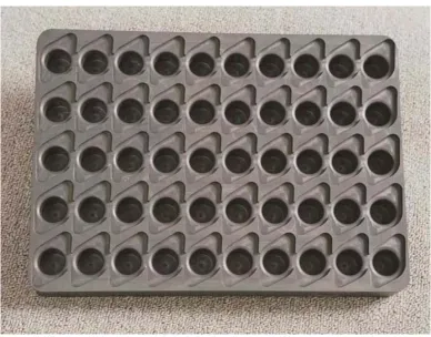
Figure 1-2 Mechanical part that has large number of pockets in it………2

Figure 2-1 Example of Zig tool path………..8

Figure 2-2 Example of Zig-Zag tool path………...8

Figure 2-3 Example of Smoot Zig-Zag tool path...…….9

Figure 2-4 Example of Contour Parallel Tool Path...…….9

Figure 2-5 Example of Spiral Tool Path………10

Figure 2-6 The curvature of line-arc-line tool paths has discontinuities at junction points, while the curvature of Bi-clothoidal splines changes continuously………14

Figure 3-1 Example of a Clothoid curve...…….19

Figure 3-2 Maximum tangent angle φ_max and angle between two linesα ………..24

Figure 3-3 Symmetric half Clothoids being used to connect two straight lines…25 Figure 3-4 Smooth corner between two straight lines formed by Clothoidal interpolation………... 25

Figure 4-1 A pocket with a convex corner ...…….28

Figure 4-2 Line-Line tool path at concave corner………28

Figure 4-3 Line-arc-line tool path at concave corner and Line-Bi-Clothoid-Line conversion………..29

Figure 4-4 Gouging due to distant Clothoid start points………31

Figure 4-5 Uncut regions at the Concave Clothoid corners……….…..32

Figure 4-7 Curve showing the change in the distance between the Clothoids

at the corners………..………….…………35

Figure 5-1 A five sided concave polygonal pocket……….……...41

Figure 5-2 Traditional boundary parallel spiral tool path for concave polygonal pocket...41

Figure 5-3 Half width cut becoming a full width cut in the corner………...42

Figure 5-4 First offset and Clothoid start points with initial Clothoids...…...43

Figure 5-5 Changing the scaling factor to connect the Clothoids...…...44

Figure 5-6 Increasing curvature of the Clothoid as the starting point is moved nearer to the corner of the offsets………..………..46

Figure 5-7 Bi-Clothoids for the second boundary offsets...…..47

Figure 5-8 The Spiral tool path with smooth corners………...47

List of Tables:

Chapter 1. INTRODUCTION

Pocket milling represents an important task in machining of mechanical parts,

dies and moulds. We propose a new method of generating boundary parallel tool paths

for 2.5D high speed pocket milling using Clothoidal Spirals. A Clothoidal Spiral also

known as Cornu Spiral or a Clothoid is frequently used in high-way design. The

curvature of the Clothoid is proportional to the length of the curve measured from the

origin of the curve. In this thesis we provide a method to generate Boundary Parallel Tool

Path with smooth Clothoid Corners for High Speed Machining. As a result of this

method, it is expected to achieve faster continuous path motion.

1.1Pocket Milling

Manufacture of various mechanical parts such as aircraft parts, molds and dies,

etc involves high intensity 2.5D pocket milling operations. In 2.5D pocket machining, a

pocket is excavated by removing layer(s) of material as shown in Figure 1.1. The tool

path for a layer of a pocket is line along which the center of the tool –an end mill, travels

as its rotating teeth cut the material. Most machining of aerospace parts can be brought of

as pocket machining [Bieterman 02]. An aerospace vehicle needs to be smooth, strong

and light weight. Pocket machining with the support structure it leaves between pockets,

helps achieve these properties. A typical example of the importance and extensiveness of

Figure 1.1 Graphical representation of pocket milling operation

Due to the large amount of pocket milling needed on many complex mechanical

parts, reducing the machining cycle time by even small amounts could bring a significant

payback. For the last few years High Speed Machining tools has been vigorously used for

large scale pocket milling operations, especially in aerospace and die/mold

manufacturing industry.

Although machine tools of very high spindle speeds are available in the market,

various machining constraints such as, motion restrictions due to pocket geometry,

motion restrictions due to the tool paths, cutting tool strength, effect of the resultant

forces on the machine tool, etc keep the users from taking use of the full capabilities of

the available High Speed Machine tools.

Tool path generation for pocket milling is mostly done with NC programming, in

which a person provides a part description and feed rate requirements to a computer aided

manufacturing software package also know as CAM. The CAM package then produces a

file with path and feed-rate data that are post processed into a form a controller can

understand and use to drive the machine tool. In this thesis, we propose a new method of

tool path planning using Clothoidal spirals for smoothening the corners, for pocket

1.2 Organization of Thesis

In Chapter 2, a survey of previous work done in high speed machining for pocket

milling and tool path generation is provided. Chapter 3 presents the definition and the

theory behind the Clothoidal spirals. In Chapter 4, we present the proposed method of

smoothing the corners of the boundary parallel offset tool paths and the algorithm used to

generate the tool path using the proposed method. In, Chapter 5 shows the computer

implementation and some practical examples are discussed. Chapter 6 presents the

Chapter 2. LITERATURE REVIEW

In this chapter we introduce, previous work done by various researchers in the

field of High Speed Machining, Pocket Milling, Tool path planning etc.

2.1High Speed Machining

High Speed Machining offers a way to mill complex structures that were never

practical before. High Speed Machining has enabled users to replace many complex

assemblies into a single machined part. Reducing the role of assembly removes cost and

lead time from the manufacturing process.

The productivity of a machining operation is often characterized by the metal

removal rate. One reason to consider high speed machining applications is to increase

productivity without sacrificing part quality. The term ‘High Speed Machining (HSM)’ is

widely accepted and common place in modern machine shops. What is ‘High Speed

Machining’?

Various sources define High Speed Machining in many different ways. High

Speed Machining is a powerful machining method that combines high feed rates with

high spindle speeds, specific tools, and specific tool motion. Typically High speed

machining uses spindles with high speed and power (generally greater than 10,000 rpm

and 10 hp) to remove metal at rates of orders of magnitude higher than by conventional

techniques. High Speed Machining addresses part design flexibility, weight savings, part

accuracy and part quality, all accomplished while maintaining a high degree of

process constraints in pocket milling the user is discouraged from taking the complete use

of the capabilities of the machine tool.

High Speed Machining makes the tool path a more significant factor in the

process. Taking lighter cuts with a smaller step-over increment is only one consideration.

An effective tool path also protects the cutting tool by keeping cutting load steady and

maintains a high feed rate by avoiding sharp changes in direction.

Decisions made during programming can also affect the quality of the work piece.

If the purpose of HSM is to machine a smooth surface, the tool path may contribute to

this goal. There are a variety of ways to machine with smoother motion. Possibilities

include rounding corners, smoothing reversals and even machining in circles.

Another approach to keeping the feed rate high doesn’t involve direction changes,

but instead involves changing the feed rate more often. Feed rate optimization may allow

the program to maintain a higher average feed rate where the profile of the cut frequently

changes.

2.2High Speed Machining and Pocket Geometry

More and more complex mechanical parts that were earlier being assembled or

manufactured by other process such as casting etc, are now being machined for various

reasons, some of which have been briefly discussed previously. Majority of these parts

require lots of pocketing operations. Pocketing operations involve removal of large

pocketing operations High Speed Machines are being used for pocket milling of complex

parts.

The complexity of the geometry of the pockets greatly reflects on the machining

speed that is achieved. Appropriate tool path planning suitable for high speed operations

is an important issue in the High Speed Machining Industry. In this report we address this

issue of improving the traditional tool paths.

2.3 Tool Path Planning

Two tool path topologies commonly used in milling operations are direction

parallel tool path and the contour parallel tool paths, also known as boundary parallel tool

paths. The direction parallel tool paths are linear tool paths that can further be classified

as, one-way or zig tool path, zig-zag tool path and smooth zig-zag. Figures 2.1, 2.2, and

2.3 show the three different types of direction parallel tool path plans.

The one-way direction parallel tool path system is a uni-directional cutting path,

and hence a consistent up-cut or down-cut chip removal can be maintained. However,

there is a considerable amount of non-productive time involved in returning the cutter to

the start- cut position at the end of each cutting path.

On the other hand, the zig-zag path is a bi-directional cutting path in which

material is removed both in the forward and the backward paths. Although the zig-zag

Figure 2.1 Example of Zig tool path

Figure 2.3 Example of Smoot Zig-Zag tool path

E1 S

P S

E

Figure 2.5 Example of Spiral tool path

up-milling and down-milling methods are alternately applied. This will lead to problems

such as machine chatter and shorter tool life.

Examples of non-linear tool paths are the contour parallel tool paths and the

parametric based tool paths. In contour parallel tool path planning, series of offset

contours of the pocket boundary are first generated. The tool travels along these offsets

one by one, until the entire pocket is machined. One method of connecting the subsequent

contours is shown in Figure 2.4 where the tool begins at the start point, S, goes around

the outermost loop, and the moves across the edge marked E1 to reach the next contour.

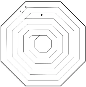
A common variation of this is spiral paths, where the move from one contour to the next

Figure 2.5), is extended outwards until it intersects the outer loop (at e.g. point P in

Figure 2.5). The tool leaves the outer loop at this point P, and moves first along the

extension to reach the inner loop.

Parametric based tool path is frequently used as a finishing tool path for

machining parametric surfaces as the tool path is driven directly along the u-v parametric

curves of the surface itself. As shown in Figure 2.4, contour parallel tool path pattern is

derived from the boundary of the concerned machining region. It is a coherent tool in the

sense that the cutter is kept in contact with the cutting material most of the time. So it

incurs less idle times such as those spent in lifting, positioning and plunging the cutter. At

the same time it can also maintain the consistent use of either up-cut or down-cut method

throughout the cutting process. Contour-parallel tool path is therefore widely used as a

cutting tool path especially for large-scale material removal. A study of machining

efficiency comparison of the direction parallel tool paths over the contour parallel tool

paths has been done by [Choi 00]. It was found that the smooth zig-zag tool path was

most efficient method, closely followed by contour parallel tool path which had sharp

corners.

The contour-parallel tool path can be divided into three different approaches: (1)

‘pair-wise intersection’ [Hansen 92], (2) ‘Voronoi Diagram’ [Persson 78], (3)

‘Pixel-based’ [Choi 97]. In the first approach, the boundaries of a machining region are offset

inwards by a step over distance. At concave corners the offset segments intersect with

each other and hence they need to be trimmed to form the resultant contour profiles. At

convex corners, the offset segments are extended and connected to produce the resultant

on each layer of the offset segments until sufficient layers of contour profiles are created

for covering the entire machining volume. However eliminating self-interactions is time

consuming and the removal of the invalid loops may lead to numerical errors.

In the second approach, individual offset segments are trimmed to their

intersections using the Voronoi diagram of the original pocket boundary. This approach

is known to be more efficient and robust since the steps in offsetting the tool path

segments can be subdivided in a more organized manner. However, as pointed out in

[Choi 99], it may also incur numerical instability if it is applied to a boundary of point

sequence curve (PS-curve) containing near circular portions.

The third approach of pixel based method requires a large amount of memory and

long computation time to achieve a desired level of precision due to its dependence on

the resolution of the Z-map.

A new pair-wise offset algorithm based on pair-wise interference detection test

was proposed in [Park 01] for removing local invalid loops from the input PS-curve

before constructing a raw offset curve. This algorithm has a near O(n) time-complexity,

where n is the number of points in the PS-curve. It can avoid the near –circular

singularity condition that exists in the traditional pair-wise approach.

No matter which one of the above three approaches is used for tool path

generation, concave and convex corners can be found in offset contours by the

intersection of the different types of geometric entities such as lines and arcs. The

corner-cutting problem provoked by concave and convex corners has not been sufficiently

produce small amount of uncut material at the corner regions when the step over is

greater than the cutter.

Also the traditional offsets contours, used directly as tool path have a drawback

because when a cutter moves into a corner region, the cutter contact length increases.

Consequently, this causes a momentary rise of cutting load, producing undesirable effects

such as shorter tool life, machine chatter and even cutter breakage. In a machining

process, it is apparent that excessive plunging and slotting, sharp velocity discontinuities,

and changing cut geometry limit production rates, increase tool wear, and reduce part

quality. To overcome some of these drawbacks, [Chan 01] have proposed a special tool

path pattern to machine a concave corner progressively using looping knots. Although the

looping knots reduce to some extent, the instant change in acceleration at the corners, the

tool path length is increased therefore affecting the efficiency of the process.

Various other researchers have worked on cutting load regularization that is

basically classified into (a) online monitoring and control and (b) prediction of cutting

loads by cutting load models as an offline approach. Tlusty and Smith (1997) address

issues of stability in end milling and the importance of the selecting the proper axial and

radial depths of cut for chatter free machining. They avoid over engagement while

cornering by adopting a spiral-in approach. Some researchers have used Bezier and

B-Spline curves for tool path generation. The Bezier and B-B-Spline curves are non-linear

functions of its parameter, hence an undesirable oscillation may occur [Walton 90].

Walton and Meek (1989) have developed methods to interpolate lines and circular

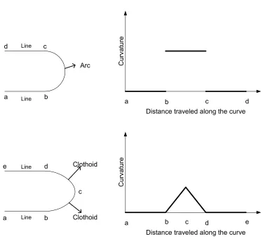
arcs with Clothoidal splines. A Clothoidal curve is unique in the sense that its curvature is

Use of Clothoidal splines in the pocket corners can therefore reduce the

drawbacks such as instantaneous variation in acceleration and feed rate at pocket corners

(Figure 2.6). a b c d a b c d e a a b b c c d d e

Distance traveled along the curve

Distance traveled along the curve

Curvatu re Cur vature Arc Clothoid Clothoid Line Line Line Line

Figure 2.6 The curvature of line-arc-line tool paths has discontinuities at junction points,

Jirawan (2003), a former member of our group had attempted to use the

Clothoidal curves for tool path generation. Jirawan’s use of Clothoids in tool path plans

showed that Clothoids allow higher feed rates and reduced total machining time. The

results of her work involved some uncut regions in the pocket between the contour

parallel offsets. To avoid the uncut regions the step distance of the contour offsets was

decreased. This resulted in longer tool path, there by affecting its efficiency.

The objective of this thesis is to design optimal contour offset tool path planning

using Clothoidal cornering that are guaranteed to avoid undercuts and gouging without

reducing the step distance.

2.4 Summary

In this chapter, various traditional tool paths were introduced. We saw that the

traditional offsets contours used directly as tool path have various drawbacks, that result

in momentary rise of cutting load, producing undesirable effects such as shorter tool life,

machine chatter and even cutter breakage. We will discuss our new method to reduce

Chapter 3. CLOTHOIDAL SPIRALS AND THEIR USE IN

GENERATING PLANAR CURVES

In this chapter, the Clothoidal curves also known as Cornu spirals are introduced.

The mathematical theory behind the Clothoidal curves and the current applications of the

Clothoidal curves are discussed. The nature of the Clothoidal curves along with its

advantages over other curves is presented. The problem for whose solution we are using

the Clothoidal curves is also introduced.

3.1 Introduction to the Problem

High Speed Machining (HSM) involves very high cutting speeds. The cutting

tool, the tool stock and the machine tool in general are affected by high forces at the

corners while making transition from one geometric shape to another due to the sudden

and irregular change in the curvature. This results in increasing wear of the cutting

tool/machine tool and hence reducing their life spans and also an inferior surface finish.

A reduction in cutting speeds at the corners will result in increased machining time,

hence reducing the efficiency.

Traditionally a pair of lines has been cornered by interpolating circular arcs

between two sides to obtain a smooth transition between the sides. Circular arc is not

sufficient for this problem because at the connecting point with the line there occurs a

discontinuous change of curvature. In the next sections of this chapter the Clothoidal

introduced. A detailed explanation of the nature of the Clothoid curves along with the

method to compute them is provided.

3.2 Clothoidal Curves

The Spiral of Cornu is named for the French scientist Marie Alfred Cornu (1841 -

1902). He studied this curve, also known as a Clothoid or Euler's Spiral, in connection

with diffraction. Euler applied a similar figure while measuring the elasticity of a spring.

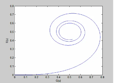
The characteristic property of Clothoid spirals shown in Figure 3.1 is that their

curvature is a linear function of the arc length, or in other words the curvature of the

curve is proportional to the length of the curve measured from the origin of the spiral.

The Clothoid is a planar curve, which is frequently used in highway and railroad designs.

A Clothoid is needed to make the gradual transition from a highway, which has zero

curvature, to the midpoint of a freeway exit, which has non-zero curvature. A Clothoid is

clearly preferable to a path consisting of straight lines and circles, for which the curvature

is discontinuous.

The generalization of the Clothoid is given by the following parametric equation

as defined in [Gray 97],

Clothoid [n, a](t) = _

           +       +

∫

∫

n u du n u a t n t n 0 1 0 1 1 cos , 1

sin (3.1)

where n is any positive natural number a and u are scaling factor and parameter,

The standard Clothoid is defined by Fresnal Integrals invented by Augustine Jean

Fresnel (1788-1827) and they are given by,

C

u

Cos

u

du

u

2

)

(

2

0

π

∫

=

du

u

Sin

u

S

u

2

)

(

2

0

π

∫

=

where u is a non-negative parameter. Plotting C (u) on the abscissa axis and S (u) on the

3.3 Computation of Fresnal Integrals

The Fresenal Integrals shown in equations (3.2 and (3.3) cannot be solved

analytically. We therefore use numerical methods to solve them. Various researchers

have proposed numerical methods to approximate the Fresnal integrals. Some of the well

known ones being from [Boersma 60, Cody 68, Hastings, Jr 56, Mielenz 97]. In this

report we use the Rational Approximations method proposed by [Heald 85] which can

approximate the Fresnel Integrals with maximum errors between _1.7×10−3_{and 4×10}−8_.

The Fresnel Integrals are recast into the polar form shown below,

)] ) ( ( 2 1 sin[ ) ( 2 1 )

(_{u R x A x x}2

C = − _lm π _jk − (3.4)

)] ) ( ( 2 1 cos[ ) ( 2 1 )

(_{u R x A x x}2

S = − _lm π _jk − (3.5)

where the R_lm and A_jk functions are rational approximations of the form,

∑

∑

0 _(3.6)

∑

∑

0 _(3.7)

An index of orthogonal error in the plane of Cornu spiral which is the diagonal

distance between approximated and exact points is given by,

( ) ( )

[

]

1 2 2

A

R δ

δ

ε = + (3.8)

where,

δR=R_lm −R₀ (3.9)

₀

(

)

1

A A R

A= π _jk −

δ (3.10)

The maximum errors within the range of _1.7×10−3_{and 4×10}−8_{have been show in}

R A

0

c =1 _{d0= 2} a₀=1 b₀=2

max

ε

1

c =0.506 d₁=2.054

2 d =1.79 1 b =2.524 2 b =1.886 3 b =0.803 3 10 7 .

1 × −

1 c =0.5083 2 c =0.3569 1 d =2.1416 2 d =1.8515 3 d =1.11021 1

a =0.1765 b₁=2.915

2 b =2.079 3 b =1.519 4 10 5 .

1 × −

1 c =0.60427 2 c =0.41159 3 c =0.1917 1 d =2.26794 2 d =2.15594 3 d =1.26057 4 d =0.60353 1 a =0.08218 2 a =0.15108 1 b =2.7097 2 b =2.3185 3 b =1.2389 4 b =0.6561 6 10 9_× −

1 c =0.698773 2 c =0.537836 3 c =0.246758 4 c =0.09458 1 d =2.40251 2 d =2.45425 3 d =1.647924 4 d =0.77829 5 d =0.297058 1 a =0.1446 2 a =0.17182 3 a =0.056405 1 b =2.83577 2 b =2.498595 3 b =1.61391 4 b =0.69638 5 b =0.28781 7 10 6_× −

1 c =0.7769507 2 c =0.6460117 3 c =0.3460509 4 c =0.1339259 5 c =0.0433995 1 d =2.5129806 2 d =2.7196741 3 d =1.9840524 4 d =1.0917325 5 d =0.4205217 6 d =0.13634704 1 a =0.1945161 2 a =0.2363641 3 a =0.068324 4 a =0.0241212 1 b =2.9355041 2 b =2.7570246 3 b =1.875721 4 b =0.978113 5 b =0.356681 6 b =0.118247 8 10 4_× −

Table 3.1 Table of values to calculate functions of rational approximations

3.4 Connecting Two Straight Lines with a Pair of Clothoidal Curves

To connect two directed straight lines, a pair of symmetrical Clothoid curves is

used [Walton 89, Makino 88]. Given two lines making an angle α in between them, a

pair of symmetric Clothoids with equal scaling parameters is used to plot a corner making

a smooth transition from the end point of the first line to the beginning point of the

second line. The two Clothoidal curves start from the end point and the beginning point

of the first and second straight lines respectively. The curves join the lines at a minimum

parameter value u= 0 i.e. the straight line and the Clothoid have the same curvature equal

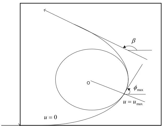
to zero at the point where they meet each other. Let u_maxbe the value of the parameter at

which the two spirals meet i.e. at the point where the curvatures of the two symmetrical

Clothoids are maximum and equal.

max

u can be calculated using the Equations (3.11) and (3.12) shown below.

2

max

β

φ = (3.11)

where φ_maxshown in Figure 3.2 is the maximum tangent angle of the Clothoid at the point

of intersection of the pair of Clothoids. β , also shown in Figure 3.2 is the maximum

tangent angle made by the complete curve (combination of both the symmetrical

Clothoids).

90

max max

φ

=

0

=

u

max

φ

max

u u =

O

β

Fig 3.2 Maximum tangent angle φ_max and angle between two linesα

An example of two straight lines connecting using a pair of symmetric Clothoid

curves is shown in Figure 3.3 and Figure 3.4. Figure 3.3 shows a pair of Clothoids

emerging from two lines making an angle α between them. The scaling factor in this

case is 1. The increase in the scaling factor results in the increase of the size of the

Clothoidal Curve. By applying the right scaling factor the pair of the half Clothoids can

Figure 3.3 Symmetric half Clothoids being used to connect two straight lines.

3.5 Summary

In this chapter the Clothoidal spirals were introduced. The method of generating

Clothoidal spirals was discussed. The definitions of Clothoidal spirals cannot be solved

numerically. Therefore a simple numerical method known as rational approximation

method that is proposed to solve the equations defining the Clothoidal spirals was

discussed. The application of these Clothoidal curves in contour parallel tool path

Chapter 4. BOUNDARY PARALLEL OFFSET TOOL PATH

GENERATION USING CLOTHOIDAL SPIRALS

The goal of this research is to use Bi-Clothoid curves to join boundary parallel

offset lines of polygonal pockets to ensure that the tool path generated has a continuous

curvature function over the entire cutting plan and the generated tool path does not leave

any uncut regions in between adjacent tool path offsets. Detailed procedure and algorithm

are presented in this chapter.

4.1 Using Clothoid Curves for High Speed Tool Machining Tool Path Generation

For the purpose of this discussion, we shall always assume that the Clothoid curve

undergoes a maximum angle of π/2. Further, in each case, the objective is to replace a

tool path sequences as per the schedule below:

Line-Line Æ Line- Bi-Clothoid – Line [Figure 4.2a]

Line-Arc-Line Æ Line – Bi-Clothoid – Line [Figure 4.2b]

In order to use these Splines, we consider two cases: Pocket corners of Concave

and Convex shapes. Details are discussed in the following sub-sections.

4.2 Tool Path Generation for Convex Corner

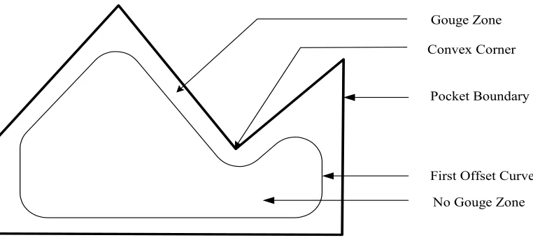
For a convex corner shown in Figure 4.1 the traditional tool path plans use

circular arc connectors between the boundary parallel offset lines to guarantee that the

tool path is _C1 _{continuous. In this work we replace the circular arc by a pair of}

symmetric Clothoids. Figures 4.2 and 4.3 show the two possible traditional tool paths at a

Pocket Boundary

First Offset Curve Gouge Zone

No Gouge Zone Convex Corner

Figure 4.1 A pocket with a convex corner

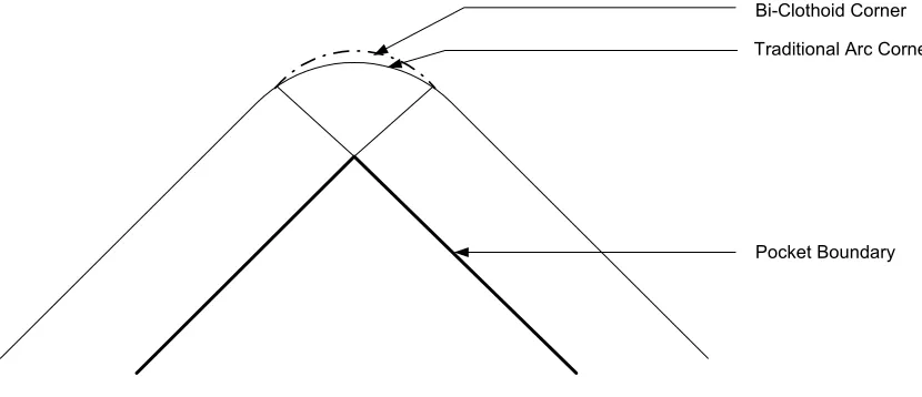
Pocket Boundary Line Line tool

path corner Convex Corner

Bi-Clothoid Corner

Traditional Arc Corner

Pocket Boundary

Figure 4.3 Line-arc-line tool path at convex corner and Line-Bi-Clothoid-Line conversion

4.2.1Lemma 1.

Replacing a Line-Line or a Line-arc-Line type of tool path at a convex corner

with a Bi-Clothoidal path will result in neither gouging, nor undercuts.

We consider the line-arc-line case. Certainly, the Clothoid cannot begin at a point earlier

than the end point of the line segment in the traditional plan. This is because moving an

infinitesimal amount along the Clothoid will result in a tool movement towards the

pocket boundary (since the clothoid has finite curvature at this point), and therefore the

4.2.2Observation 1.

A Bi-Clothoid(a pair of symmetrical Clothoids) constructed as described earlier

([Chapter 3]), and starting precisely where the circular arc begins does not

intersect the circular arc. It is easy to see that initially, the clothoid has curvature

smaller than that of the interpolating circular arc, and hence travels to the interior

of the pocket, away from the circular arc as shown in Figure 4.3.

The curvature,c_v, of the clothoid is given by

a u

c_v =π (4.1)

where a is the scaling factor and u is the parameter.

Since a is computed numerically for different values of tool radius, R, and

included angle,α , therefore one can plot ‘safe’ regions (values of R and α ) for which we

can replace precisely the circular arc with a bi-clothoid without any gouging.

For an unsafe combination of R andα , the Clothoid intersects with the circular

arc resulting in gouging. This is shown in the Figure 4.4. In such a case, we need to

continue along the straight line a little further, before we embark upon the clothoid. i.e.

the starting points of the Clothoid are to be taken closer to the corner to obtain a gouge

Circular arc Clothoid Start

Point

Clothoid crossing circular arc

α

α

Figure 4.4 Gouging due to distant Clothoid start points.

4.2.2 Observation 2.

Since the convex pocket corner is machined precisely by the offset lines, thus in

both the above possibilities, there will be no undercut at a convex corner.

4.3 Tool path generation for Concave corner

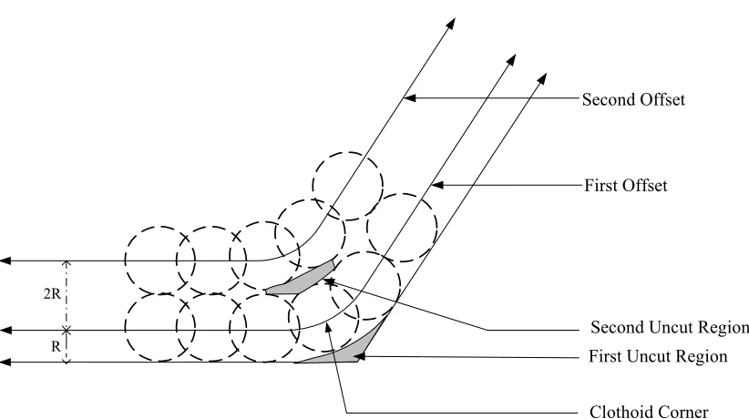
We now focus our analysis to concave corners. In this case, due to the geometry,

it is possible that the designed Clothoids may leave some un-cut material in the interior of

the pocket as shown in Figure 4.5 (Second uncut region). Such un-cut regions are

obviously undesirable.

First Uncut Region Second Uncut Region First Offset

Second Offset

2R

R

Clothoid Corner

Fig 4.5 Uncut regions at the Concave Clothoid corners

In this section, we shall concentrate on the proper selection of Bi-Clothoids that

can avoid such uncut regions. There are two ways to solve this problem.

One way is that, we can reduce the offset distance until there is no remaining

uncut area. However, this approach will result in (possibly) more number of offsets and

therefore increase the resulting tool-path’s length and machining time. We therefore

concentrate on the other way which involves selecting a proper Clothoid for the corners

It is clear that in any scheme, there is some area at the pocket boundary corners as

shown in Figure 4.5 (First uncut region) due to the cylindrical shape of tool. This is

usually removed by the finishing operations. Our goal is to ensure that the subsequent

uncut areas are completely eliminated.

To analyze this we shall distinguish between the first offset and the subsequent

offsets.

4.3.1 First offset curve

The only decisions are the selection of the start point of the Clothoid, and,

subsequently, the determination of the scaling factor. The start point is user defined based

on the tool size and the machine tool capabilities. The amount of leftover material (first

uncut region) at the pocket corners that will be removed in the finishing operation shown

in Figure 4.5 is also taken into consideration while deciding the start points for the

Clothoids of the first boundary offset.

4.3.2Subsequent Offset Curve

Let A and A′ be the starting points of the Clothoid cornering the first and

subsequent offset lines respectively as shown in Figure 4.6. Let B be a point on the inner

A

B A′ First Offset

Second offset

Pocket Boundary

Figure 4.6 Clothoid start point search on second offset

A reasonable location for the Clothoid starting point A′ is beyond point B on the

inner offset. Any Clothoid starting before B will leave some uncut region between the

first offset and the subsequent offset of the type ‘second uncut region’ shown in Figure

4.5

Consider an arbitrary location for A′ on the subsequent offset beyond B as shown

in Figure 4.6. Let R be the perpendicular distance between the first and the second

offsets. As we proceed along the Clothoid starting fromA′, the distance between the two

offsets gradually reduces to a value below R (distance between parallel offsets) along the

R

M

Q L

Figure 4.7 Curve showing the change in the distance between the Clothoids at the

corners.

that the Clothoid starting point A′lies beyond point B, hence, there is a certain delay in

the curvature of second offset Clothoid starting from A′ as compared to the outer offset

Clothoid starting from A.

Now since the curvature of the Clothoid on the second offset is greater then the

curvature of the Clothoid on the first offset, because of the smaller scaling factor, the

higher curvature of the Clothoid on the second offset (starting from pointA′) overrides

the initial delay factor as we proceed further along the length of the first offset Clothoid

corresponding to the curve beyond point M inFigure 4.7 thereby gradually increasing the

distance between the two Clothoids of the offsets to a value more then R.

Therefore the starting point for the Clothoid for an inner offset should lie at some

distance away from the corner such that the connecting point between two symmetrical

But a point very close to L on curve part Q in figure (4) means that the starting

point A′is too close to the corner of the second offsets resulting in a very small radius of

curvature at the corner which will cause a jerk effect on the machine tool. It is therefore

obvious that the starting point A′ should lie at such a location which will result in the

longest possible curve part Q in Figure 4.7 and A′corresponds to point M in Figure 4.7.

4.4 Proposed Clothoid Curve Tool Path Generation Algorithm

Based on the discussions provided in this chapter we now propose a Clothoid

curve tool path generation algorithm that uses the Bi-Clothoids to obtain a smooth,

Clothoid Curve Tool Path Generation Algorithm

Input

Polygonal Pocket Geometry Cutting tool diameter, d

Initial Scaling Factor (Default Scaling Factor is 1)

Output

Boundary Parallel Offset tool paths Start

Step 1. Calculate the slopes and angles formed by all the sides of the polygon Step 2. Generate first boundary parallel offset polygon with a step distance of d/2 Step 3. Generate subsequent successive boundary offsets with step distance, d

Step 4. Calculate the starting point of the Clothoids at each corner of the first offset polygon.

Typically the distance for starting point of this Clothoid =2*d. It is also affected by the machine tool specifications and the amount of corner left over material that will be removed in the finishing operations.

Step 5. Calculate the value of the maximum parameter,u_max for all of the corners

on the first boundary offset using Equation 3.12

The value of the u_maxremains the same for the entire subsequent

boundary offsets.

Step 7. Check if the symmetric Clothoids meet, if yes, proceed to Step 8, else proceed to Step 7.1

Step 7.1 Increase the scaling factor if the symmetric Clothoids cross each other or decrease the scaling factor if the symmetric Clothoids are short of meeting each other.

Step 7.2 Recalculate the Clothoids and repeat Step 7 until the symmetric Clothoids meet.

Step 8. Repeat Step 6 for all the corners of the boundary offset.

Step 9. Search for Clothoid starting point on the second boundary offset point. Step 9.1 Select a corner of the second boundary offset

Step 9.2 Initial Clothoid starting point for the respective corner is a point on the second boundary offset that is normal to the starting point of the Clothoid on the first boundary offset

Step 9.3 Calculate the symmetric Clothoids

Step 9.4 Check if the symmetric Clothoids meet, if yes, proceed to step 10, else, change the parameter as explained in Step 7.1 and repeat the process from Step 9.3.

Step 10 Verify for any islands of the type second uncut region shown in Figure 4.4 and explained in Case 4.3.2. If there is no island proceed to Step 11, else, proceed to Step 10.1

Step 10.1 As explained in Case 4.3.2, move the starting point further towards the corner of the second boundary offset and repeat the process from Step 9.3

Step 12. Consider the next boundary offset (third boundary offset) and let, First boundary offset = Second boundary offset,

Second boundary offset = Third boundary offset. Repeat the procedure starting from step 9.

Step 13. Repeat the Steps 9 to 12 until the corner Clothoids for all the boundary offsets have been calculated.

Step 14. Plot the offsets with the continuous corners formed by Clothoids. End

The above presented algorithm can be used to generate smooth Clothoid curve

tool paths for 2.5D high speed milling of polygonal pockets. With the smooth curvature

transition at the corners formed by the Bi-Clothoids, the generated tool paths can be used

for high speed machining with lesser acceleration variation of the cutter and the resultant

Chapter 5. COMPUTER IMPLEMENTATION AND

EXAMPLES

In this chapter, the computer implementation of the proposed boundary offset tool

path generation algorithm using Clothoidal curves is demonstrated. A step-by-step

explanation of the tool path generation process is explained along with some

computer-generated images of the tool path.

5.1 Computer Implementation

The proposed algorithm was implemented in MATLAB Version 6.5 programming

tool. The program was run on a 1.63 GHz personal computer.

For a concave pocket example we considered polygonal pocket geometry of five

sides shown in Figure 5.1. The tool path was generated using a cutting tool of radius 0.25

inches.

The traditional boundary offset spiral tool path for this kind of pocket in Figure

5.1 is shown in Figure 5.2. It can be clearly seen in the traditional tool paths that the

corners make extremely sharp turns. As the cutting tool moves into these sharp corners,

the acceleration of machine has to be instantly reduced resulting in a jerk motion effect

on the machine tool. The radial depth of cut and chip sizes increase rapidly at the sharp

corners. The cutting force and material removal rate is also very high in these areas which

tend to reduce the productive life of the cutter and the machine tool. We expect our

method of corner smoothing with the help of Clothoidal spirals will reduce all the above

0 2 4 6 8 10 12 14 16 18 20 22 -2

0 2 4 6 8 10 12

Figure 5.1 A five sided concave polygonal pocket

0 2 4 6 8 10 12 14 16 18 20 22 -2

0 2 4 6 8 10 12

For our discussion we will consider only one corner of the polygonal pocket to

demonstrate how the tool path was generated. The same process can be repeated for each

of the corners to obtain the complete tool path. The maximum parameter, u, for the given

dimensions of the pocket was calculated to be equal to 0.5.

For High Speed Machining it is important to use the full tool diameter for the

width of cut in pocketing. Any smaller width of cut will strain the tool, because width of

cut will increase as the tool enters a corner as shown in Figure 5.3. For example, a

half-width cut becomes a full-half-width cut in the corner. Therefore An offset distance of 0.5*d,

where d is the diameter of the cutting tool, was taken for the first offset.

Depth of Cut

Depth of Cut

Stock Removed

The offset distance for the subsequent offsets is taken as diameter d. The starting

point for the pair of Bi-Clothoids which is user defined as taken at a distance of 2*d on

the offset lines from the corner. The first offsets along with the initial Bi-Clothoids for

an initial scaling factor of a=1, is shown in Figure 5.4.

Figure 5.4. First offset and Clothoid start points with initial clothoids.

Since the two initial Clothoids do no meet each other the scaling factor is

gradually increased until the Clothoids just meet at the ends. . If the initial Clothoids over

cross each other, the scaling factor is gradually decreased till they just meet at the ends.

The behavior of the initial clothoid with the gradual increase in scale factor is shown in

Figure 5.5. Note that when the scaling factor is increased the curvature of the clothoids is

a u

c_v =π (5.1)

where scaling factor a is in denominator, thereby increasing the curvature, c_v every time

the scaling factor is decreased.

Figure 5.5. Changing the scaling factor to connect the Clothoids

In Figure 5.7, the second boundary offset is shown along with the Bi-Clothoids at

the corner. Initial starting points for the Bi-Clothoids were the points lying on the second

offset which are normal to the starting points on the first offset. The Bi-Clothoids starting

from the initial starting points tend to leave some uncut region. This is because the

Clothoids on the second offsets have higher curvature due to lower scaling factor. The

curl of the Clothoids on the first boundary offsets. As a result the distance between the

uncut Clothoids of first boundary offset lines and the Clothoids of the second boundary

offset lines is more at the tips of the Clothoids as compared to the start point of the

Clothoids.

To avoid this kind of uncut region the Clothoids have to be moved further near to

the corner as explained in the previous chapter. An example indicating the behavior of

the Bi-Clothoid as it’s starting point is moved nearer to the corner is show in Figure 5.5

In Figure 5.7 this is shown by another Clothoid on the second boundary offset which is

slightly nearer to the corner as compared to the initial Clothoid that was plotted on the

second boundary offsets. This new Clothoid is also tested for any uncut regions. The

testing is done by measuring the distance between the connecting point of the

Bi-Clothoids on the second boundary offsets and the connecting point on of the Bi-Bi-Clothoids

on the first boundary offsets. As discussed in the previous chapter the distance between

these Bi-Clothoid connecting points tends to be the maximum. If this maximum distance

is lesser then or equal to the offset distance d, then it indicates that there is no uncut

region in that corner and therefore the current pair of Bi-Clothoids can be accepted as the

tool paths cornering the current boundary offset lines. Similarly Bi-Clothoids are

calculated for all the corners for the current offset as well as the subsequent offsets.

Figure 5.8 shows the contour parallel spiral tool path for the polygonal pocket

shown in Figure 5.1 developed using the proposed algorithm. The entire boundary

smooth continuous corners. Figure 5.9 shows another example of smooth cornered tool

path for a polygon.

Figure 5.6 Increasing curvature of the Clothoid as the starting point is moved nearer to

Figure 5.7. Bi-Clothoids for the second boundary offsets.

Figure 5.8 The spiral tool path with smooth corners

Figure 5.9 Another example of spiral tool path with smooth corners

5.2 Summary

In this chapter the implementation of our proposed algorithm for using Clothoidal

splines (Bi-Chlothoids) for contour parallel tool path cornering was demonstrated. Tool

path by the proposed method for an example part has also been presented. The important

Chapter 6. CONCLUSION

6.1 Conclusion

In this paper a new and non conventional method to generate contour parallel

offset tool paths for 2.5D pocket milling has been introduced. We have used the

Clothoidal curves which have traditionally been used in the Highways and Rail tracks

construction to replace the sharp corners in 2.5D polygonal pockets.

The proposed algorithm to generate the new type of tool path has been discussed.

The algorithm presented does not leave any uncut regions in between the contour parallel

offset tool paths. The algorithm uses an iterative method to determine suitable symmetric

Bi-clothoids to make sure that no uncut regions are left behind in the interior of the

pocket. To reduce the number of iterations needed to determine the right Clothoids a start

point of search was identified based on certain logical observations.

The proposed algorithm was programmed and run on example polygonal pockets

to generate a spiral tool path. The resultant corners are smooth and continuous in nature.

The unique property of the linear curvature variation along the length of curves will be

extremely useful for high speed motion of the cutting tool along the corners of these

pockets. The smooth Clothoidal Corners are intended to result in smoother machine tool

acceleration and deceleration at the corners as compared to conventional Circular Arc

Corners. The stresses and forces induced on the cutter and the machine tool spindle will

corner resulting in longer cutting tool and machine tool, life. Better acceleration at the

corners will also help in reducing the overall cycle times of machining.

6.2 Future Work

The proposed method can be further extended for pockets of more complex

boundaries, pockets with islands, etc. Methods for connecting other geometric curves

such as a circle with a circle or a line with a circle have already been published been

published by [Meek and Walton, 1989] giving us an opportunity to try more complicated

pocket geometries. There is also a lot of scope to combine this method of tool path

generation with online federate optimization to take maximum use of the capabilities of

the available high speed machine technology.

The proposed method may also be useful in Robots for painting and welding

References

1. Bae S, Ko K, Kim B, Choi B, “Automatic federate adjustment for pocket

milling”, Computer-Aided Design vol.35, (2003), 495-500.

2. Bieterman M and Sandstrom D, “A curvilinear tool-path method for pocket

machining”, Proceedings of IMECE 2002, ASME, Nov 17-22, 2002, New

Orleans, Louisiana, USA.

3. Boersma J, “Computation of Fresnel Integrals,” Math. Comp, vol. 14, (1960), p.

380.

4. Chan K W and Choy H S, “A corner looping based tool path for pocket milling”,

Computer Aided Design, vol.35, (2001), 155-166.

5. Choi B K and Kim B H, “Die Cavity pocketing via cutting simulation”, Computer

Aided Design, vol.29, no.12, (1997), 837-846.

6. Choi B K and Kim B H, “Machining efficiency Comparison, Direction parallel

with contour parallel tool path”, Computer Aided Design, vol.34, (2002), 89-95.

7. Choi B K and Park S C, “A pair-wise offset algorithm for 2D point-sequence

curve,” Computer Aided Design, vol.31, no.12, (1999), 735-745.

8. Choi B K and Park S C, “Uncut-free pocketing tool paths generation using

pair-wise offset algorithm,” Computer Aided Design, vol.33, no.10, (2001), 739-746.

9. Cody W J, “Chebysev approximation for the Fresnel Integrals,” Math. Comp, vol.

22, (1968), 450-453

10.Dagiloke I, Kaldos A, Douglas S, Mills B, “High speed machining: an approach

to process analysis”, Journal of Materials Processing Technology, 54, (1995),

11.Dey T, Zhao W, “Approximate medial axis as a Voronoi sub complex”,

Computer-Aided Design, (2003)

12.Fallbohmer P, Altan T, Tonshoff H, Nakagawa T, “Survey of the die and mold

manufacturing industry’, Journal of Materials Processing Technology, vol. 59,

(1996), 159-168

13.Farouki R, Tsai Y, Wilson C, “Physical constraints on federates and feed

accelerations along curved tool paths”, Computer-Aided Design vol.75, (2000),

337-359.

14.Flutter A, Todd J, “A machining strategy for tool making”, Computer-Aided

Design vol.33, (2001), 1009-1022.

15.Gray A, Modern Differential Geometry of Curves and Surfaces with

Mathematica, Second Edition, (1997), 64-66.

16.Hansen A and Arbab F, “An algorithm for generation of NC tool paths for

arbitrarily shaped pockets with islands”, ACM Trans Graph , Vol.11,

No.2,(1992), 152-158.

17. Hastings C, Jr, “Approximations for calculating Fresnel Integrals,” Math. Comp.

[MTAC], vol. 10, (1956), p. 173.

18.Hatna A, Grieve R, Broomhead P, “Automatic CNC milling of pockets: geometric

and technological issues”, Comp. Intergraded Manufacturing Systems, vol.11, No.

4, (1998), 309-330.

19. Heald M, “Rational Approximations for Fresnel Integrals,” Math. Comp, vol. 44,

20. Heald M, “Rational Approximations for the Fresnel Integrals”, Mathematics of

Computation, Vol.44, Issue 170 (1985), 459-461.

21.Held M, “Voronoi Diagrams and offset curves of curvilinear polygons”,

Computer-Aided Design vol.30,no.4, (1998), 287-300.

22.Held M, Lukacs G, Andor L, “Pocket machining based on contour –parallel tool

paths generated by means of proximity maps”, Computer-Aided Design

vol.26,no.3, (1994), 189-203.

23.Held M, “VRONI: An engineering approach to the reliable and efficient

computation of the Voronoi diagrams of points and line segments”,

Computational Geometry, vol.18, (2001), 95-123.

24.Ibaraki S, Ogawa T, Matsubara A, Kakino Y, “Model based learning of cutting

forces in end milling processes”, Japan-USA Symposium of Flexible Automation,

(2002)

25.Jayaram S, Kapoor S, DeVor R, “Estimation of the specific cutting pressures for

mechanistic cutting force models”, International Journal of Machine Tools and

Manufacture, vol. 41, (2001), 265-281.

26.Kakino Y, Saraie H, Ohtsuka H, Nakagawa H, “Intelligent end milling system and

its application to internal cylindrical machining with spiral curves”, Japan-USA

Symposium of Flexible Automation, (2002)

27.Klaus D M, “Computation of Fresnel Integrals,” J. Res. Natl. Inst. Stand. Techno.

vol.102, (1997), p. 363

28.Ko J, Yun W, Cho D, “Off-Line feed rate scheduling using virtual CNC based on

29.Lee E, “Contour offset approach to spiral tool path generation with constant

scallop height”, Computer-Aided Design vol.35, (2003), 511-518.

30.Makino H, “Clothoidal Interpolation – A New Tool for High-Speed Continuous

Path Control”, Annals of CIRP, vol. 37, no. 1, (1988), 25-28.

31.Meek D S and Thomas R S D, "A guided clothoid spline", Computer Aided

Geometric Design vol.8, (1991), 163-174.

32.Meek D S and Walton D J, "Offset curves of Clothoidal splines",

Computer-Aided Design 22(1990), 199-201.

33.Meek D S and Walton D J, "The use of Cornu spirals in drawing planar curves of

controlled curvature", Journal of Computational and Applied Mathematics

25,(1989), 69-78.

34. Narita H, Shirase K, Wakamatsu H, Tsumaya A and Arai E, “Autonomous

milling process control based on real time cutting simulation”, Japan-USA

Symposium of Flexible Automation, (2002)

35.Otsuka H, Yamazi I, Ito T, Ihara Y, Kakino Y, Matsubara A, “Advanced feed

forward control for constant cutting forces in die machining”, Japan-USA

Symposium of Flexible Automation, (2002)

36.Park S, “Tool-path generation for Z-constant contour machining”,

Computer-Aided Design vol.35, (2003), 27-36.

37.Park S, Choi B, Chung Y, “Contour-parallel offset machining without

tool-retractions”, Computer-Aided Design vol.35, (2003), 841-849.

38.Persson H., “NC machining of arbitrarily shaped pockets”, Computer Aided

39.Renton D, Elbestawi M A, “ High speed servo control of multi axis machine

tools”, International Journal of Machine Tools and Manufacture, vol. 40, (2000),

539-559

40.Richards N, Fussel B, Jerard R, “Efficient NC machining using off-line optimized

feedrates and on-line adaptive control”, Symposium on Process Planning and

Process Optimization, (2002), IMECE, New Orleans, 1-11.

41.Roth D, Ismail F, Bedi S, “Mechanistic modeling of the milling process using an

adaptive depth buffer”, Computer-Aided Design,vol.35, no.14, (2003),

1287-1303.

42.Stori J A and Wright P K, “A constant engagement offset for 2-1/2D tool path

generation”, Proceedings of the ASME, MED, vol.8, (1998), 475-481.

43.Tlusty J and Smith S, “Current trends in high speed machining”, Transactions of

ASME, vol.119, (1997), 664-666.

44.Walton D J and Meek D S, "Clothoidal splines", Computers and Graphics vol.14,

(1990), 95-100.

45.Wang J, Ravani B, “Computer aided contouring operation for traveling wire

electric discharge machining (EDM)”, Computer-Aided Design vol.35, (2003),

925-934.

46.Wang L, Miura K, Nakmae E, Yamamoto T, Wang T, “An approximation

approach of the clothoid curve defined in the interval [0, pi/2] and it’s offset by

free form curves”, Computer-Aided Design, vol.33, (2001), 10419-1058.

47.www.mathworld.wolfram.com

49.Xu H, “Line and angular federate interpolation for planar implicit curves”,

Computer-Aided Design vol.35, (2003), 301-317

50.Yong T, Narayanaswami R, “A Parametric interpolator with confined chord

errors”, acceleration and deceleration for NC machining”, Computer-Aided

Design, (2003).

51. Zhang L, Fhu J, Nee A, “Tool path regeneration for mold design modification”,

Computer-Aided Design vol.35, (2003), 813-823.

52.Zhao M, Balchandran B, “Dynamics and stability of milling process”, Intl. J.