ABSTRACT
ZHOU, QUAN. Wireless Communications with MIMO Systems: Analysis and Practice. (Under the direction of Dr. Huaiyu Dai).
WIRELESS COMMUNICATIONS WITH MIMO SYSTEMS:
ANALYSIS AND PRACTICE
by QUAN ZHOU
A dissertation submitted to the Graduate Faculty of North Carolina State University
in partial fulfillment of the requirements for the degree of
Doctor of Philosophy
ELECTRICAL ENGINEERING
Raleigh 2006
APPROVED BY:
_________________________________ _________________________________ Huaiyu Dai Brian L. Hughes
Chair of Advisory Committee
_________________________________ _________________________________
Keith Townsend Alexandra Duel-Hallen
BIOGRAPHY
Quan Zhou received his B.E. degree in Communication and Control from Northern Jiaotong University, Beijing, China, in 1998. And he received his M.E. degree in Electronic Engineering from Tsinghua University, Beijing, China in 2001. In August 2001, he started his graduate studies at North Carolina State University in the Department of Electrical and Computer Engineering. His research interests are in the areas of wireless MIMO communications with emphasis on link adaptation and multiuser MIMO network. His current research focuses on nonlinear optimization in wireless communication systems with emphasis on crosslayer optimization.
ACKNOWLEDGMENTS
My graduate study at North Carolina State University is one of the most memorable periods of my life. I have benefited tremendously from my interactions with many extraordinary individuals. First of all, I would like to thank my advisor Professor Huaiyu Dai for his supervision, support and encouragement throughout my Ph.D. research. I sincerely appreciate his help in suggesting research topics, revising papers and solving some critical problems during my research. I am very glad to be one of his first students.
I would also like to thank my committee members Professor Keith Townsend, Professor Brian Hughes and Professor Alexandar Duel-Hallen for their expertise and advice. I learned the fundamentals of communication and signal processing theory through their classes. Their way of teaching showed me an excellent example of a systematic and straightforward fashion in presenting technical ideas. I would also like to thank Professor Jack. W. Silverstein and Professor Zhidong Bai for their helps in providing some proofs in chapter 4.
It was a great pleasure to have closely worked with my colleagues: Dr. Jia Liu, Hongyuan Zhang, Wenjun Li, Xingying Yu and Li Ma. I thank them for the numerous suggestions, guidance, comments, and enlightening discussions.
TABLE OF CONTENTS
LIST OF FIGURES ... viii
LIST OF TABLES ...ix
1. INTRODUCTION ...1
1.1 Overview of wireless MIMO communications ...1
1.2 Outline of the Thesis...3
1.3 List of author’s publication...4
2. Asymptotic Symbol Error Rate of MIMO Spatial Diversity System...6
2.1 Background...6
2.2 System Model...7
2.3 Asymptotic Average Symbol Error Rate ...9
2.4 Summary...14
3. Joint Antenna Selection and Link Adaptation for MIMO Systems...15
3.1 Background...15
3.2 Problem Formulation ...17
3.2.1 MIMO Systems with Transmit Antenna Selection...17
3.2.2 ZF-SIC with QR Decomposition Interpretation...18
3.2.3 Joint Antenna Selection and Link Adaptation...18
3.3 Joint Antenna Selection and Link Adaptation for uncorrelated MIMO Channels ....22
3.3.1 Incremental Selection Rule with Link Adaptation ...22
3.3.3 Simplified Link Adaptation for Uncorrelated Rayleigh MIMO Channels ...26
3.4 Joint Antenna Selection and Link Adaptation for Correlated MIMO Channels ...28
3.4.1 Correlated MIMO Channels...28
3.4.2 Antenna Selection and Link Adaptation Only Based on Channel Correlation Information ...29
3.5 Numerical Results...33
3.6 Summary...45
4. Asymptotic Analysis on the Interaction between Spatial Diversity and Multiuser Diversity in Wireless Networks ...46
4.1 Background...46
4.2 Joint Spatial Diversity and Multiuser Diversity System ...48
4.3 Asymptotic System Capacity and Scheduling Gain as K Goes to Infinity while M Keeps Fixed ...50
4.4 Asymptotic Scheduling Gain as M Goes to Infinity while K Keeps Fixed ...56
4.5 Scheduling Gain when both M and K Goes to Infinity ...62
4.6 Summary...67
5. Joint Tomlinson-Harashima Precoding and Scheduling for Multiuser MIMO with Imperfect Feedback ...68
5.1 Background...68
5.2 THP and Multiuser Scheduling for downlink MIMO...69
5.2.1 THP for multiuser MIMO ...70
5.3.1 Channel Prediction via LRP ...75
5.3.2 Actual Achievable Rate under Imperfect CSI...75
5.4 Numerical Results...77
5.5 Summary...80
6. Conclusions and Future Work ...81
BIBLIOGRAPHY ...84
APPENDIX...90
APPENDIX A: Some proofs of chapter 2...91
APPENDIX B: Some proofs of chapter 3...93
LIST OF FIGURES
Figure 2.1 Comparision between asymptotic and simulated results for BPSK under
different antenna configurations ... 10
Figure 2.2 The value of α varies with number of transmit antennas under the same M×N ... 11
Figure 2.3 Symbol error rate of the three spatial diversity schemes under BPSK ... 11
Figure 3.1 Antenna selection gain and link adaptation gain ... 34
Figure 3.2 Performance comparisions of the proposed algorithms in 6x6 MIMO with throughput 12bits/s/hz ... 36
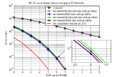
Figure 3.3 Performance comparisons of the proposed algorithms in 16x16 MIMO with throughput 32bits/s/hz ... 38
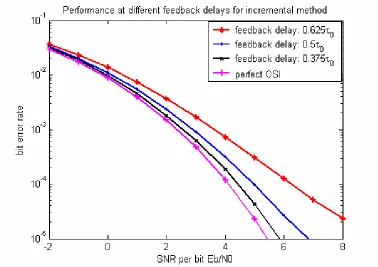
Figure 3.4-a Performance with different feedback delays for incremental methods... 39
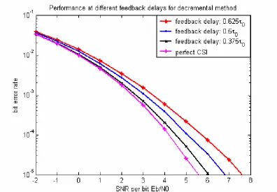
Figure 3.4-b Performance with different feedback delays for decremental methods... 40
Figure 3.5-a Joint antenna selection and link adaptation for fading correlation scenario 1... 41
Figure 3.5-b Histogram of the number of active antennas for fading scenario 1 ... 42
Figure 3.6-a Joint antenna selection and link adaptation for fading correlation scenario 2... 42
Figure 3.6-b Histogram of the number of active antennas for fading scenario 2 ... 43
Figure 3.7-a Joint antenna selection and link adaptation for fading correlation scenario 3... 43
Figure 3.7-b Histogram of the number of active antennas for fading scenario 3 ... 44
Figure 4.1 Average system capacity of opportunistic scheduling (γt=0 dB M, = =N 2).. 55
Figure 4.2 Average throughput of round robin scheduling (SNR=0dB)... 60
Figure 4.3 Scheduling gain as the number of antennas grows (SNR=0dB, K=50)... 61
Figure 4.4 Scheduling gain as both the number of antennas and users grow (SNR=0dB,K=M)... 66
Figure 4.5 Scheduling gain as the number of antennas and users grow (SNR=0dB, K=exp(M)) ... 67
Figure 5.1 Block diagram of the proposed THP for multi-user MIMO downlink ... 72
Figure 5.2 Performance comparison of different scheduling scheme ... 79
LIST OF TABLES
Table 3.1 Incremental antenna selection rule with link adaptation for uncorrelated
MIMO……….24
Table 3.2 Decremental antenna selection rule with link adaptation for uncorrelated
MIMO……….25
Table 3.3 Incremental antenna selection rule with link adaptation for correlated
MIMO……….32
Table 3.4 Fading correlation scenarios……….40 Table 3.5 Active antenna index and constellation carried by each active
Chapter 1
INTRODUCTION
1.1 Overview of wireless MIMO communicationsThe use of multiple antennas at both the transmitter and receiver side, so as to form a multiple-input multiple-output (MIMO) antenna system, is an emerging technology that makes building both reliable and high data rate wireless networks a reality [17][56]. Compared with the conventional single-input single-output (SISO) system, MIMO system creates multiple spatial dimensions that can be exploited to improve the performance1 of the wireless link. More specifically, such performance improvement comes from the array gain, diversity gain, multiplexing gain and interference cancellation introduced by MIMO systems, which are illustrated below.
Array gain is achieved by using multiple antennas at the transmitter and receiver so that the received signals can add coherently. To exploit the transmit/receive array gain, transmitter/receiver needs to have the channel state information (CSI). The transmit/receive array gain is proportional to the number of transmit/receive antennas.
independently fading paths created by multiple antennas. A well-known example to exploit the spatial diversity gain without CSI at the transmitter side is space-time coding, like the Alamouti code for two transmit antennas [2]. For a MIMO system with M transmit antennas and N receive antennas, a maximum spatial diversity order of M×N can be achieved.
In a rich scattering environment, MIMO channels can offer a linear (min
(
M N,)
) increase in capacity with the number of antennas without increasing the transmission power or bandwidth. The spatial multiplexing gain can be realized by transmitting and receiving parallel independent streams across the multiple antennas at both ends; a famous example is the pioneer Bell Labs Layered Space-Time (BLAST) architecture proposed by Foschini in [18].. An interesting tradeoff between the spatial diversity gain and multiplexing gain is revealed in [74].In cellular communications, cochannel interference arises due to frequency reuse. Multiple antennas can be used in cellular communications to mitigate the cochannel interference thus increasing the reuse factor and improving the system capacity. The basic idea is to make use of the spatial channel response (usually a vector) between the desired user and interference users, and design the receive weighting vector to maximize the signal power to interference power ratio.
1.2 Outline of the Thesis
Our thesis focuses on the four interesting topics on MIMO systems, which is organized as follows.
In chapter 2, through the analysis of the probability distribution function (PDF) of the received signal to noise ratio (SNR), we study the asymptotic symbol error rate of point-to-point MIMO spatial diversity system. The results reveal a simple connection with system parameters, providing good insights for the design of MIMO diversity systems.
In chapter 3, in order to protect the transmitted data against random channel impairment in wireless MIMO communications, we consider link adaptation, such as rate adaptation and power control to improve the system performance and guarantee certain quality of service. We propose a joint antenna subset selection and link adaptation study for MIMO systems, including both uncorrelated and correlated MIMO channels. Specifically, we propose one simplified antenna selection and link adaptation rule based on the expected optimal number of active antennas for uncorrelated MIMO with Rayleigh fading, and one for correlated MIMO channels only based on the slowly varying channel correlation information. Our proposed algorithms demonstrate significant gains over traditional MIMO signaling while feasible for practical implementation through numerical results.
that reveal inter-connections and fundamental tradeoffs among key system parameters are given, which afford us some insights in real system design.
In chapter 5, we propose a crosslayer approach that explores Tomlinson-Harashima Precoding (THP) at the physical layer to reduce the multiuser scheduling burden at the MAC layer, and improves the sum rate of the downlink multiuser MIMO systems. Our proposed scheme is further evaluated with imperfect feedback, obtained by the long range prediction (LRP) technique. Compared to some existing scheduling schemes, the proposed scheme approaches the performance upper bound in certain scenarios, while incurring much less computation complexity. Significant gains are still maintained with imperfect channel state information (CSI), fed back at a rate much lower than the data rate.
Finally, in chapter 6, we propose some open problems and future work of our thesis. 1.3 List of author’s publication
Below are the publications during the author’s Ph.D. research: Journal publications:
[J1] Q. Zhou and H. Dai, “Joint Antenna Selection and Link Adaptation for MIMO Systems,” IEEE Transactions on Vehicular Technology, vol. 55, no. 1, pp.243-255, Jan. 2006.
[J2] Q. Zhou and H. Dai, “Asymptotic Analysis on the Interaction between Spatial Diversity and Multiuser Diversity in Wireless Network,” submitted to IEEE Transactions on Signal Processing, Dec. 2005 (under second review).
[J3] Q. Zhou and H. Dai, “Asymptotic Analysis in MIMO MRT/MRC systems,” submitted to EURASIP Journal on Wireless Communications and Networking, Jan. 2006.
Conference publications:
[C2] Q. Zhou and H. Dai, “Asymptotic Analysis on Spatial Diversity versus Multiuser Diversity in Wireless Networks,” Proc. IEEE International Conference on Communications (ICC), Istanbul, Turkey, June 2006.
[C3] Q. Zhou, H. Dai and H. Zhang, “Joint Tomlinson-Harashina Precoding and Scheduling for Multiuser MIMO Downlink with Imperfect Feedback,” Proc. IEEE Wireless Communications and Networking Conference (WCNC), Las Vegas, NE, Apr. 2006. [C4] H. Dai, and Q. Zhou, “Asymptotic Analysis in MIMO Diversity Systems,” Proc.
International Symposium on Intelligent Signal Processing and Communication Systems (ISPACS), HK, CHINA, Dec. 2005.
[C5] Q. Zhou and H. Dai, “Joint Antenna Selection and Link Adaptation for MIMO Systems,” Proc. 2004 Fall IEEE Conference on Vehicular Technology (VTC), Los Angels, CA, Sept. 2004.
Chapter 2
Asymptotic Symbol Error Rate of MIMO Spatial Diversity System
2.1 Backgroundkeeps fixed, the antennas distribution with M −N minimized will provide the lowest SER, while the other is that when M ×N is fixed, a distribution with maximum M +N gives the best performance. But the authors do not provide a rigorous justification for both observations. Some similar observations are also made in [36].
This chapter is organized as follows. In Section 2.2, we will give our model for MIMO MRT/MRC systems. Then we provide our asymptotic analysis for the average SER in Section 2.3 and Section 2.4 respectively, together with some numerical results for illustration purpose. Final conclusion is made in Section 2.5.
2.2 System Model
We assume a narrowband MIMO diversity system with M transmit antennas and N
receive antennas, modeled as:
, tu
= + = +
y Hx n Hw n (2.1)
where M 1
t
×
∈
w £ is the unit-norm transmit weight vector and u is the transmitted symbol with power PT, N×1
∈
y £ is the received vector, N M×
∈
H £ is the channel matrix, and N×1
∈
n £
is a zero-mean circularly symmetric complex Gaussian noise vector with variance 2 / 2
n
σ per
real dimension. We define γt =PT/σn2 the average transmit SNR. For illustration purpose, independent and identically distributed Rayleigh fading is considered for H, but our analysis can be readily extended to other fading scenarios when appropriate distributions are available. When multiple MIMO users are involved, their channels are assumed independent.
At the receiver side a weight vector N 1
r
×
∈
right and left singular vector corresponding to the largest singular value σmax of H to maximize the output SNR.
The cumulative distribution function (CDF) of 2 max
x =σ is given by [37]
/
1
( )
( ) , (0, ),
( 1) ( 1)
MRT MRC c
s k
x
F x x
t k s k
γ
=
= ∈ +∞
Π Γ − + Γ − +
Ψ
(2.2)
where s =min(M N, ), t=max(M N, ), and Ψc( )x is an s s× Hankel matrix function with the
( , )thi j entry given by {Ψc( )}x i j, =γ(t− + + −s i j 1, )x , for ,i j=1, 2,...,s. Here γ( , )a β is the incomplete Gamma function defined as 1
0
( , )a βe tt a dt
γ β = − −
∫
, and Γ( )a is the Gammafunction defined as Γ( )a =γ( ,a +∞). The probability distribution function (PDF) of x can be derived as
/ 1
( ) ( ) ( ( ) ( )), (0, ), MRT MRC
c c
fγ x =F x tr Ψ− x Φ x x∈ +∞ (2.3)
where Φc( )x is an s s× matrix whose ( , )thi j entry is given by
{
}
2 ,( ) t s i j x
c x i j x e
− + + − −
=
Φ .
selected so that the resultant channel gain is maximized. This scheme requires less feedback than the MIMO MRT/MRC.
In the remainder part of this chapter, we write ( ) ~g x f x( ) if
0 ( )
lim 1
( ) x
or x
g x f x
→∞ →
= .
2.3 Asymptotic Average Symbol Error Rate
In this section, we will derive a succinct expression for average SER at high SNR. The conditional SER for lattice-based modulations can be represented by the Gaussian tail Q -function as Ps( )H =M Qn ( κγtx) , where Mn is the number of the nearest neighboring constellation points, and κ is a positive fixed constant determined by the modulation and coding schemes [55]. At high transmit SNR γt, the system performance will be dominated by the low-probability event that x becomes small [63]. Therefore, only the behavior of
/ ( ) MRT MRC
fγ x at x→0+ determines high transmit SNR performance. To find the asymptotic expression for Ps =E P{ ( )}s H at high γt, we need the following result for the behavior of
/ ( ) MRT MRC
fγ x at the origin.
Lemma 1:
1
/ 0 1
1 0
!
( ) ~ , as 0
( )! s
MRT MRC k MN
s k
MN k
f x x x
t k
γ
−
− +
= − =
→ +
∏
∏
.Proof: See Appendix A.
With Lemma 1, we establish the following result for the asymptotic average SER for MIMO MRT/MRC systems following Proposition I in [63].
Proposition 1: For MIMO MRT/MRC systems, the asymptotic average SER is given by
( / ) ( / ) ( / ) ( / )
( 1) ( 1)
( / )
3
2 ( )
2 ( ) ( ).
( 1)
MRT MRC MRT MRC
q MRT MRC MRT MRC n
q q
s MRT MRC t t
M q
P o
q
α
κγ γ
π
− + − +
Γ +
= × +
+ (2.4)
where 1
( / ) 0 ( / )
1 0
!
, 1.
( )! s
MRT MRC k MRT MRC s
k
MN k
q MN
t k
α
− = − =
= = −
+
∏
∏
(2.5)The validity of (2.4) is demonstrated in Figure 2.1 for uncoded BPSK systems. Based on (2.4), one readily concludes that the optimal diversity order for MIMO diversity systems is
M ×N. Therefore, if we keep M +N fixed (a measure of system cost), even distribution of
Figure 2.2 The value of α varies with number of transmit antennas under the same
M×N
the number of transmit and receive antennas (more precisely a smallest M −N ) maximizes
M×N, thus minimizing the system SER at high SNR. On the other hand, when comparing two MIMO MRT/MRC systems with the same diversity orderM×N, the one with smaller
(MRT MRC/ )
α yields larger coding gain and thus smaller SER (in this case, q(MRT MRC/ ) is a constant). We can conclude that in this scenario, the sum of transmit and receive antennas should be made as large as possible, with the optimum achieved at s=1 and t=M ×N. This conclusion is based on the following result regarding (MRT MRC/ )
α as a function of M and N
(or equivalently of s and t).
Lemma 2: Given four positive integers s1, t1, s2, t2, assume s1× = ×t1 s2 t2, s1<t1 , s2<t2, and s1+ > +t1 s2 t2, then α(MRT MRC/ )( , )s t1 1 <α(MRT MRC/ )( , )s t2 2 .
Proof: see Appendix A.
From the asymptotic SER expression in (2.4), we have verified the two observations made in [13] rigorously at high SNR. In what follows, we will compute the corresponding parameters for the coding gain and diversity order for MIMO STBC/MRC and SC/SC systems (whose asymptotic average SERs assume the same forms as (2.4)).
STBC/MRC
Without loss of generality, we assume that the adopted space-time block coding scheme achieves the full rate and the transmit power is equally allocated among the transmit antennas. In this case, the normalized effective link SNR for a generic user is given by
2 , 1 1 1 N M
i j i j
h M
γ
= =
/ 1
( ) , 0.
( 1)!
MN
STBC MRC M MN Mx
f x x e x
MN
γ = − − − ≥ (2.6)
Therefore the corresponding parameters for the coding gain and diversity order for MIMO STBC/MRC systems can be obtained following a similar approach as above as
( / ) ( / )
, 1.
( 1)!
MN
STBC MRC M STBC MRC
q MN
MN
α = = −
− (2.7)
SC/SC
In this spatial diversity scheme, both the user and the base station choose one optimal antenna such that the resultant channel gain is maximized. Thus the normalized effective link SNR at the receiver is
( )
, 21i Nmax,1 j M hi j γ
≤ ≤ ≤ ≤
= , whose PDF can be easily obtained as
/ 1
( ) (1 ) , 0.
SC SC x x MN
fγ x =MNe− −e− − x≥ (2.8)
We can obtain the corresponding parameters for the coding gain and diversity order for MIMO SC/SC systems as
( / ) ( / )
, 1.
SC SC SC SC
MN q MN
α = = − (2.9)
Comparing (2.5), (2.7) and (2.9) we can see that all these MIMO diversity schemes achieve the same diversity order. Nonetheless, their error performances could still be dramatically different owing to different coding gains, as exhibited in Figure 2.2. For example, when M =6 and N =1, our formulas predict a SNR gap of 4.7 dB between MRT/MRC ( ( / )
1/120
MRT MRC
α = ) and SC/SC ( ( / ) 6
SC SC
well with simulation results (see Figure 2.3 at SER 10−5). It is also observed that for the same diversity order, the performance of STBC worsens with the increase of transmit antennas. 2.4 Summary
Chapter 3
Joint Antenna Selection and Link Adaptation for MIMO Systems
3.1 BackgroundThe use of multiple antennas at both the transmitter and receiver side, so as to form a multiple-input multiple-output (MIMO) antenna system, is an emerging technology that makes building high data rate wireless networks a reality [19][58]. Transmitting independent data streams simultaneously from different antennas through spatial multiplexing (see, e.g., [1]) effectively realizes the high spectral efficiency promised by MIMO systems, but leaves the transmitted data unprotected from random channel impairment. Therefore, it is often desirable to consider link adaptation, such as rate adaptation and power control to improve the system performance and guarantee certain quality of service [8][76][14][49].
One of the drawbacks with an MIMO system is the increased complexity and hardware cost due to the expensive RF chains required by each active antenna. It is of increasing research interest recently to find a good antenna selection scheme that can significantly reduce such cost while incurring little performance loss. Generally, there are two goals for antenna subset selection in MIMO systems: one aims to maximize the channel capacity [26][46], the other aims to minimize the bit error rate for spatial multiplexing systems when some practical signaling schemes are used [24][25][32][47].
subchannel gains (post-detection signal-to-noise ratio (SNR)) are determined by the active antenna subset, while some weak subchannels are naturally dropped during link adaptation process. Motivated by this fact, we propose a joint antenna subset selection and link adaptation study for MIMO systems.
In a real propagation environment, the capacity of a MIMO system may be lower than what is predicted with rich scattering assumption due to fading correlation [51][10]. Meanwhile, link adaptation and antenna selection are expected to achieve more gains in correlated MIMO channels due to more prominent subchannel discrepancies. Furthermore, fading correlation information varies much more slowly, hence it is feasible and advantageous to implement antenna selection and link adaptation only based on the correlation information rather than on the instantaneous channel information. The author in [48] also proposed some simplified rules for joint antenna selection and link adaptation based on the channel correlation information, aiming to maximize some lower bounds of the minimum post SNR. Therefore the performance of these rules depends on how tight the lower bounds would be. Furthermore, the exhaustive search entailed there might make these rules still complex in implementation.
This chapter is organized as follows. In Section 3.2, we introduce the MIMO system model with transmit antenna selection, and formulate the problem of joint antenna subset selection and link adaptation. In Section 3.3, we develop incremental and decremental antenna selection rules with link adaptation for uncorrelated MIMO channels. We also propose a simplified rule based on the expected optimal number of active antennas to further reduce complexity. In Section 3.4, we develop an antenna selection rule with link adaptation for correlated MIMO channels only based on the slowly varying channel correlation information. Simulation results are given and analyzed in Section 3.5. Finally, in Section 3.6, we make conclusions and propose some future work.
3.2 Problem Formulation
3.2.1 MIMO Systems with Transmit Antenna Selection
Without loss of generality, we assume a narrowband MIMO system with total Kt
transmit and Nr receive antennas, with the channel between Kt transmit and Nr receive antennas denoted by H. In our study, the antenna selection is only carried out at the transmitter side, and it is easily shown that the best performance is achieved when all receive antennas are active [50]. With Nt out of Kt transmit antennas to be chosen, we denote the selected subset of transmit antennas by p and the channel matrix between the selected Nt
transmit antennas and Nr receive antennas by H(p), whose columns correspond to the selected antennas. The received signals are then given by
( )p ,
= +
y H x n (3.1)
where ( ,1 2,..., )
t
T N
x x x
=
x is the transmitted signal vector, ( ,1 2,..., )
r
T N
y y y
=
y is the received signal vector, and ( ,1 2,..., )
t
T N
n n n
=
n is assumed to be i.i.d Gaussian with zero mean and variance of σn2. For ease of description, we will drop the index pin (3.1) in the following discussion when no ambiguity incurs. All through this paper we assume Nr ≥Nt.
3.2.2 ZF-SIC with QR Decomposition Interpretation
The zero-forcing successive interference cancellation, widely used in MIMO detection, can be simply interpreted by matrix QR decomposition. With H=QR, where Q is a unitary matrix and Ris an upper triangular matrix, we can apply QH to the received vector to obtain y% =Q yH =Rx+n% , detailed as
1,1 1,2 1,
1 1 1
2 2,2 2, 2 2
, ...
0 ...
,
: : : : : : :
0 0 ..
t t
t t t t t
N N
N N N N N
r r r
y x n
y r r x n
y r x n
= + % % % % % % (3.2)
from which the transmitted symbols , 1,..., 1
t t
N N
x x − x can be detected successively. Assume no error propagation during interference cancellation process2, it is clear that QR decomposition decomposes an Nr×Nt MIMO channel matrix H into Nt subchannels with ri i, being the gain for the ith subchannel.
3.2.3 Joint Antenna Selection and Link Adaptation
As mentioned in the introduction, the link adaptation problem and the antenna selection problem are often coupled for a MIMO system. Furthermore, it is often beneficial
2
to use only a good subset of antennas in MIMO communications to reduce hardware complexity and energy consumption. The induced performance loss is often negligible when judicious antenna selection is made and link adaptation is employed. To this end, we propose to jointly consider the antenna selection and link adaptation for wireless MIMO communications. Antenna selection and link adaptation can be realized either at the transmitter or at the receiver, depending on the availability of channel state information. In the latter case, the receiver will only feed back the selected active antenna subset and corresponding communication modes to the transmitter.
In this chapter we assume QAM modulation for illustration purpose. For square M -ary QAM with average power γ , the minimum Euclidean distance d is
6 , 1
d M
γ
=
− (3.3)
which is also a good approximation for energy efficient “non-square” QAM in a large range of interest [1].
Assume there are Nt active antennas in use. For the ithsubchannel with gain ri,i , the
square of the minimum Euclidean distance of the output constellation is given as 2
, 2
, 6
, 1, 2,..., , 1
i i i
i out i
i
r
d i N
M
γ
= =
− (3.4)
{
}
1 1 2 , {1,... } ( , , , ): ,max min ,
Nt
Nt t
t i i i i T i T i
i out i N N p b b b
d γ = γ γ = ∈ = = ∑ ∑ (3.5)
where bi =log2 Mi is the number of bits allocated to the i−th subchannel, bT and γT are the total throughput and power constraints imposed on the system.
In (3.5) we want to find an optimal antenna subset together with its optimal bit and power allocation, subject to the total throughput and power constraints. The number of active antennasNt can also be an optimization parameter, thus further complicating the problem. To our best knowledge, the global optimal solution is open and often a thorough search has to be resorted to, which is typically infeasible for practical implementations. Therefore we take some effective steps to decouple the original problem into some suboptimal ones, which will be shown to yield excellent performance nonetheless.
First, assuming the set of active antennas and associated bit allocation are given, as the system performance is limited by the worst subchannel, to maximize the aggregate performance we would like to allocate power so as to achieve the same output minimum Euclidean distances for all subchannels, i.e., 1,2 ... 2 , ( )2
t
out N out e
d = =d =d , given as
2 ( )
2 1 2
, ,
1 1
6
. 6
( ) ( 1)
1
t t
T T
e N N
j j j j j
j j j
d
r r M
M γ γ − − = = = = × × − −
∑
∑
(3.6)Thus our optimization goal is simplified as 2
, 1
min ( 1) min ( ), ( ) ,1 ,
t
N
j j j t t t t
j
r − M N N N K
=
× − = ≤ ≤
∑
g m (3.7)subject to log (2 1) log (2 2) ... log (2 )
t
T N
where ( ) ( 1,1 2, 2,2 2,..., , 2)
t t
T
t N N
N = r − r − r −
g is named the antenna gain vector, while
1 2
( ) ( 1, 1,..., 1)
t
T
t N
N = M − M − M −
m is named the bit allocation vector, and g denotes the inner product between them. Our target is to find an optimal pair of
(
g(Nt),m(Nt))
for a given Nt, and further choose the best pair among 1≤Nt ≤Kt, when the number of active antennas is not given beforehand.Given Nt , the optimal pair of
(
g(Nt),m(Nt))
can be found through a thorough search in principle, which is still not an easy task when Nt and Kt are large. We further decouple the antenna selection and bit allocation problems by exploiting the discrete and finite-alphabet nature of the bit allocation vector m(Nt).When the total throughput and the modulation set are given, the possible choices of the bit allocation vector can be determined in advance by a lookup table. Furthermore, by Lemma 3 given in the appendix B, in order to minimize (3.7), only one permutation (decreasing order) of the elements in the bit allocation vector needs to be considered for each possible combination. With this decoupling, the optimization problem is finally approximated as an antenna selection problem to find a suitable (g Nt) followed by table lookup to find a matching m(Nt). Some simple recursive algorithms are proposed in the next section to avoid exhaustive search while incurring little performance degradation.of M-ary PSK with powerγ is given byd 2 sin (2 )
Mπ γ
= . Correspondingly, (3.7) becomes
2 2 ,
1
min csc ( )
t
N j j
j j
r
M
π
−
=
×
∑
subject to the same constraint.3.3 Joint Antenna Selection and Link Adaptation for uncorrelated MIMO Channels We first consider the uncorrelated MIMO channels where the channel matrix H can be modeled with i.i.d. complex Gaussian entries. Two basic recursive algorithms are proposed to choose the desired antenna gain vector (g Nt): incremental selection means the
“desired” antennas are recursively added to an initially empty active antenna set while decremental selection means “undesired” antennas are recursively removed from an initially full antenna set3. When Nt <<Kt, we can use the incremental selection rule described in Section 3.3.1, while we can use the decremental rule in Section 3.3.2, when Nt is close to
t
K . In a general link adaptation problem where Nt is unknown in advance, we can search over all possible 1≤Nt ≤Kt to find the optimal one. To reduce complexity, we propose an adaptive selection rule based on estimation of Nt in Section 3.3.3.
3.3.1 Incremental Selection Rule with Link Adaptation
Intuitively, we want r1,1 , r2,2 , …, rN Nt, t as large as possible. Our incremental recursive rule works as follows: starting from a column of H (Nr×Kt) which results in maximum r1,1 (corresponding to the largest vector norm), we successively choose from the remaining columns of H such that the next subchannel gain is maximized. The subchannel
3
gain of the newly added antenna can be obtained in a closed-form solution, which is described by the following lemma.
Lemma4.a Assume the QR decomposition of a matrix H( )k with kindependent columns is ( )
( ) ( ) k
k k
=
H Q R . Then for the enhanced matrix H(k+1) = H( )k h with QR decomposition ( 1)
( 1) ( 1) k
k k
+ = + +
H Q R , the first k diagonal elements of R(k+1) keep the same with those of R( )k , while the (k+1)th one is given by h hH −h QH ( ) ( )k Q k Hh; similarly, the first k column vectors of Q(k+1) keep the same with those of Q( )k , while the (k+1)th one is
given by
1
(:, 1) (:, ) (:, ) k
H l
k l l
=
+ = −
∑
Q h Q hQ .
Proof: see the appendix B.
Based on Lemma 4.a, assume in the kth step, H( )k stores the kselected columns of H and the QR decomposition of H( )k is Q(k)R(k), then in the (k+1)th step, we choose the column vector h from ( )
\ k
H H (which represents the remaining columns ofH) in such a way that r 1, 1 h h h Q(k)Q (k)h
H H
H k
k+ + = − is maximized. Furthermore, it can also be shown as follows that the successively generated antenna gains are already ordered.
Lemma4.b In the above incremental selection rule for uncorrelated MIMO,
1,1 2,2 , ,
| | .. ...
t t
k k N N
r ≥ r ≥ ≥ r ≥ ≥ r .
Proof: see the appendix B.
Lemma 4.b shows that the elements in the selected antenna gain vector 2
2 2
1,1 2,2 ,
( ) ( , ,..., )
t t
T
t N N
N = r − r − r −
arrange the elements of candidate bit allocation vectors m(Nt) in a deceasing order in the lookup table according to Lemma 1, which saves storage space and increases the matching speed for (3.7). We further assume mˆ(Nt) is the optimal bit allocation vector that minimizes
(Nt), (Nt)
g m for a given g(Nt).
The incremental selection rule with link adaptation for uncorrelated MIMO is summarized in the following table.
Table 3.1 Incremental antenna selection rule with link adaptation for uncorrelated MIMO
Set I={1,2,3,..,Kt} and p=Φ(empty set),g=Φ(empty set), Q=Φ(empty set) for i=1 to Kt
αi = H(:, )i 2; end
1 (1) arg max
t
i i Kα
≤ ≤
=
p , 1,12
1 max t i i K r α ≤ ≤
= ,g(1)=1/r1,21, Q(:,1)=H(:,p(1))/ H(:,p(1);
I=I p\ (1);
for k =2 to Nt
update α αi = i− H(:, )i HQ(:,k−1)2, for all i∈I;
( ) arg max i i k α ∈ = I p ; 2 , max
k k i
i r α ∈ = I ; 2 , / 1 )
(k = rkk
g ; 1 1 (:, ) (:, ( )) (:, ) (:, ( ) (:, ) k H l
k k l k l
−
=
= −
∑
Q H p Q H p Q ;
; ) (:, / ) (:, )
(:,k Q k Q k
Q =
) (k
p I
I= − ;
end
assume
( )
ˆ( ) arg min ( ), ( )
t
t t t
N
N = N N
m
m g m ;
(1: t)
Two points are noteworthy for the above algorithm. First, due to Lemma 4.a and 4.b, the antenna selection and link adaptation process is significantly expedited. Secondly, due to the recursive nature of the algorithm, searching an optimal Nt for a general link adaptation problem does not mean Kt times of effort (as calculation for Nt+1 is just one step further based on calculation for Nt), but rather the worst-case effort where all Kt transmit antennas must be deployed. Nonetheless, in case nearly all the Kt transmit antennas would be deployed, we provide a decremental selection rule for link adaptation, which is described in the following subsection.
3.3.2 Decremental Selection Rule with Link Adaptation
Set H(Kt) =H;
Using [30] to find square root of
(
(H(Kt))HH(Kt))
−1, assume P(Kt) =(
(H(Kt))HH(Kt))
−1/ 2;Assume ( )
( )
1
ˆ arg min t ,: t
K l K
l l
≤ ≤
= P ( P
( )
l,: means the length of the lth row), discard the lth ˆ column of H(Kt), assume the deflated matrix to be H(Kt−1);for k =1 to Kt −(Nt+1)
Using [30] to find square root of (H(Kt−k)HH(Kt−k))−1, based on P(Kt− +k 1);
assume P(Kt−k) =(H(Kt−k)HH(Kt−k))−1/ 2 ;
Discard the lth column of ˆ H(Kt−k), whereˆ argmin ( )
( )
,:1 l
l k
k l≤ P
≤
= ,
assume the deflated matrix to be H(Kt− −k 1);
end
Compute the sorted antenna gain vector g(Nt) for (Nt) H ; assume
( )
ˆ( ) arg min ( ), ( )
t
t t t
N
N = N N
m
m g m ;
(Nt)
return H and mˆ(Nt);
The decremental selection rule with link adaptation for uncorrelated MIMO is summarized in Table 3.2. Our proposed decremental selection rule is related to the V-BLAST ordering rule first proposed in [61], which successively chooses the antenna (among those not already chosen) that maximizes post-detection SNR under the assumption of perfect feedback. Accordingly, we can successively discard the antenna (among those not already chosen) that minimizes the post-detection SNR under the assumption of perfect feedback. Usually repeated matrix inversion will be involved during the process of discarding, which may introduce much computation complexity and numerical instability. Thanks to the work in [30], we can avoid computing the inversion of the deflated channel matrix by means of a recursive square-root algorithm.
3.3.3 Simplified Link Adaptation for Uncorrelated Rayleigh MIMO Channels
In a general link adaptation problem where Nt is not fixed in advance, we need to test all possibilities 1≤Nt ≤Kt to find the optimal one using either the incremental or decremental selection rule. In this subsection, we propose a simplified selection rule based on the estimation of the optimal number of active transmit antennas to further reduce the complexity. With i.i.d. complex Gaussian channel matrix, ri i, 2 in (3.7) is a
2
χ distributed
random variable with 2 (× Nr+ −1 i) degrees of freedom [8], where the probability density function of the χ2distribution with v degrees of freedom is given as:
( 2) / 2 / 2 / 2
( | ) ,
2 ( / 2)
v x
v
x e
f x v
v
− −
=
Γ (3.8)
where ( )Γ x is the gamma function defined as 1 0
( )x ∞tx− −e dtt
Γ =
∫
.The expected value of 1/ri,i 2 can be obtained as
0
1/( 2) 2
1
( | ) .
2
v for v
f x v dx
for v
x
+∞ − >
= +∞ =
∫
(3.9)Replacing 1/ri,i 2 in (3.7) with their expected values, we have
(
)
1 1
min ( ), ( ) min ( 1),1
2( )
t
N
t t j t t
j r
E N N M N K
N j
=
= × − ≤ ≤
−
∑
g m (3.10)
subject to
2 1 2 2 2 1 2
log ( ) log ( ) ... log ( ) and .
t t
T N N
b = M + M + + M M ≥M L≥M (3.11)
Therefore, we can estimate the optimal number of active antennas in a pre-processing stage as follows: for all possible bit allocation vectors m(Nt) 'sthat satisfy (3.11), find the one that minimizes (3.10), denoted asmˆ(Nt); then find
1
ˆ
arg min ( ), ( )
t t
t t t
N K
N E N N
≤ ≤
= g m
% ,
which is our estimate of the optimal number of active antennas in i.i.d Rayleigh fading MIMO channels. Thus we can decide to use either the incremental or decremental selection rule for joint antenna selection and link adaptation for different system settings based on the value of N%t. Furthermore, we can restrict ourselves to search optimal Nt only in the range around N%t to further reduce the computational complexity. Simulations results show that searching Nt in the range of N%t −1,N%t+1 and storing only three bit allocation vectors
ˆ(Nt−1)
3.4 Joint Antenna Selection and Link Adaptation for Correlated MIMO Channels 3.4.1 Correlated MIMO Channels
In this section, we extend the study of joint antenna selection and link adaptation to correlated MIMO channels. We assume correlation only exists at the transmitter side, as described by the “one-ring” model in [51]. This model is feasible, e.g., for the outdoor macrocell situation where the transmitter at the base station is elevated high above the local scattering environment, while there are sufficient local scatters around the mobile receivers. For an Nr ×Kt MIMO system, the channel can be modeled as H=HwATH
with H T
T
T A R
A * = , where Hw is an Nr ×Kt matrix containing i.i.d. complex Gaussian random variables and RT is a Kt×Kt Hermitian semi-positive definite matrix representing the covariance matrix for each row of H.
Again, we assume Nt out of Kt antennas are to be selected. As before, the channel matrix between the Nt transmit antennas and Nr receive antennas can be described as H(p)=Hw(p)ATH(p), where p contains the indices of the selected antennas, and
) ( ) ( )
(p TH p T p
T A R
A = is the corresponding submatrix of RT.
We assume uniform linear arrays at both the transmitter and receiver, with antenna spacing ∆T (relative to the carrier wavelength). We also assume there are L clusters of scatterers in the environment and the angle of departure for the l−th path cluster is Gaussian distributed as θl ~N(θl,σl2). Then the ( , )i j −th entry of the transmit covariance matrix
2 1
(2 ( ) sin( ) ) 2 ( ) cos( ) 2
, , .
T l l T l i j
j i j
T l i j e e
π θ σ
π θ − − ∆
− − ∆
≈
R (3.12)
For a narrowband system, the net correlation matrix can be obtained by summing the covariance matrices contributed by the L clusters weighted by the fraction of power in the corresponding cluster. As a counterpart to (3.1), the received signal in correlated MIMO can be written as:
( ) H( ) . w p T p
= +
y H A x n (3.13)
Clearly, joint antenna selection and link adaptation algorithms described in the previous section can be readily applied to correlated MIMO channels and are expected to achieve more substantial gains. However it is noteworthy that for correlated MIMO, the elements of H(p)
T
A vary much more slowly than those of Hw(p) , which is mainly determined by the local physical parameters, such as antenna spacing and angle spread. Since these parameters are relatively static and can be measured more accurately than instantaneous channel information, antenna selection and link adaptation based on ATH(p) is more attractive than that based on (p) H(p)
T w A
H . Targeting on this goal, in the next subsection, we will describe a joint antenna selection and link adaptation algorithm for correlated MIMO only based on the channel correlation information.
3.4.2 Antenna Selection and Link Adaptation Only Based on Channel Correlation Information
By applying QR decomposition successively to the correlation matrix ATH( )p =Q R1 1 and Hw( )p Q1=Q R2 2, (3.13) becomes
.
= +
Apply QH2 to the received vector, we have
2 2 1 .
H
= = +
y% Q y R R x n% (3.15)
The optimization goal for correlated MIMO channels is given as (cf. (3.2) and (3.7)):
1 2 2 1
min | ( , ) ( , ) | ( 1) min '( ), ( )
t
N
j t t
j
j j j j − M N N
=
× − =
∑
R R g m (3.16)
subject to log (2 1) log (2 2) ... log (2 )
t
T N
b = M + M + + M ,
with
2 2
1 2 1 2
'( ) (1,1) (1,1) ... ... ( , ) ( , ) T
t t t t t
N = − N N N N −
g R R R R (3.17)
and
1 2
( ) ( 1, 1,..., 1)
t
T
t N
N = M − M − M −
m
the corresponding antenna gain vector and bit allocation vector for correlated MIMO. Since the distribution of HwQ1 is the same as Hw, 2
2
|R ( , ) |j j is still χ2
distributed with degree of freedom 2×(Nr +1− j). In order to derive an antenna selection and link adaptation rule only based on RT, we replace |R2( , ) |j j −2 in (3.17) with their expected values (see (3.9)) to get
2 2
1(1,1) 1( , )
( ) ... ... .
2( 1) 2( )
T t t t
r r t
N N N
N N N
− − = − − R R g (3.18)
Hence (3.16) is turned into:
2 1
1
| ( , ) |
min ( 1) min '( ), ( )
2( )
t
N
j t t
j r
j j
M N N
N j − = × − = −
∑
Rg m (3.19)
subject to. log (2 1) log (2 2) ... log (2 )
t
T N
In recognition of R1H*R1 =AT( )p ATH( )p =RT( )p , for correlated MIMO, our goal is to find a submatrix of RT whose Cholesky factor will provide a close-to-minimization result of (3.19).
Similar to Section 3.3.1, we decouple the antenna selection and link adaptation problems and present an incremental selection rule as follows. Starting from an empty set, in each step we would like to choose from the remaining components of RT such that the next subchannel gain is maximized. This process is expedited by the following lemmas.
Lemma5.a Assume matrix RT(k) is Hermitian positive definite with size k, whose Cholesky decomposition is given by RT(k) =R(k)HR(k) , then for the enhanced matrix
=
+
1 ) ( ) 1 (
H k T k
T
v v R
R with Cholesky decomposition RT(k+1) =R(k+1)HR(k+1) , the first k
diagonal elements of R(k+1) { }, k1 i i i
r = keep the same with those ofR( )k , while the (k+1)th
one is given by 1, 1 1 v
( )
R( ) 1v− +
+ = − Tk
H k
k
r .
Proof: see the appendix B.
Based on Lemma 5.a, assume in step k, there are k selected transmit antennas, and )
(k T
R is the k×k covariance matrix for those k selected transmit antennas, which is guaranteed to be invertible according to our selection rule, then in step k+1, we will choose the antenna whose covariance vector v will maximize 1, 1 1 v
( )
R( ) 1v− +
+ = − Tk
H k
k
r . Note that
antennas jointly by means of maximizingr2,2, i.e., choose the first two active antennas whose corresponding Cholesky decomposition will result in maximization of r2,2. Also note that the condition number of RT is high, hence we can set a positive threshold value C0 in practice to discard those essentially zero-gain subchannels.
Similar to Lemma 4.b, the following lemma facilitates the optimization of (3.19). Lemma5.b In the above incremental selection rule for correlated MIMO, r1,1≥...rk k, ≥rk+ +1,k 1. Proof: See the appendix B.
___________________________________________________________________________
Set I:={1,2,3,..,Kt} and p:=Φ(empty set), T:=Φ(empty set)
(
1 1)
, 1 max arg ) 2 : 1
( v v
p H
j i −
= ,T(1):=1,
(
1 1)
, 1 max : ) 2
( v v
T H
j i −
= , where v1 =RT(i,j) and j
i≤ ;
I:=I−p(1)−p(2); for k =3 to Nt
Ak−1:=RT(p(1:k−1))(Submatrix of RTdesignated byp(1:k−1) ); ( ) max
(
1 −1 −1−1 −1)
∈ −
= k k
H k I
j
k v A v
T ;
( ) argmax
(
1 −1 −1−1 −1)
∈ −
= k k
H k I
j
k v A v
p , where vk−1 =RT(p(1:k−1),p(j))(The column
vector in p(j)column and p(1:k−1)rows of RT
); I:=I−p(k);
if , ˆ( 1)
) 1 : 1 ( 1 ) 1 ( 1 ) ( ˆ , ) : 1 ( 1 1 − − − − >
−k k k N k k k
Nr r
m T
m
T
return p(1:k−1) and mˆ(k−1)
else if T(k)≤C0 (C0 is a threshold value) break;
else if k=Nt
return p(1 :Nt) and mˆ(Nt)
end
end
Lemma5.b shows the elements in '(g Nt) are already in an increasing order. Thus we only need to arrange the elements of candidate bit allocation vectors m(Nt) in a deceasing order according to Lemma3. In summary, the incremental selection rule with link adaptation for correlated MIMO is described in Table 3.3. For correlated MIMO, a decremental selection rule is usually not necessary, since the ill-conditioning of the channel matrix typically results in much fewer antennas being selected as opposed to the uncorrelated MIMO of the same size. Furthermore, antenna selection and link adaptation modes need to be updated only when the channel covariance matrix changes, which happens far less frequently compared to that based on the instantaneous channel fading.
Similarly, in a general link adaptation problem where Nt is unknown in advance, we can search over all possible 1≤Nt ≤Kt to find the optimal one.
3.5 Numerical Results
In this section, we evaluate the performance of our proposed joint antenna selection and link adaptation algorithms for both uncorrelated and correlated MIMO channels through several representative examples. Square QAM modulation is employed in all simulations with 256-QAM the largest constellation to be used.
random antenna selection; the second one is V-BLAST with a selected transmit antenna subset obtained through the incremental selection rule; and the last one is our proposed incremental antenna subset selection with link adaptation given in Table I. Link adaptation based on singular value decomposition (SVD) of the channel matrix [75] is also included, which can be viewed as a performance upper bound since the decomposed subchannels are truly interference free. From Figure 3.1, we can see that antenna selection gain is dominant, while link adaptation gain is also significant especially at high SNR (by observing the difference of the slope of the third curve (diversity gain) from that of the second one, and its similarity with that of the upper bound curve).