Tropical Atlantic Vertical Wind Shear Variability in a Future Climate

(1)

TALGO, KEVIN D. Tropical Atlantic Vertical Wind Shear Variability in a Future Climate. (Under the direction of Assistant Professor Anantha R. Aiyyer).

Simulations from a suite of 21 fully-coupled global climate models (GCMs)

col-lected for the International Panel on Climate Change’s Fourth Assessment Report

(IPCC-AR4) provide a unique opportunity to explore the effects of climate change on tropical

cyclone (TC) activity. Vertical wind shear is a key environmental variable that has a

detri-mental effect on the genesis and intensification of TCs. Variability of shear in the Atlantic

is influenced by changes in the large-scale background circulation, forced by teleconnections

such as the El Ni˜no-Southern Oscillation and the West African monsoon system.

Spatio-temporal variability of ENSO and West African (Sahel) rainfall in the 20th

century is examined for the suite of GCMs. This serves as a basis to determine which models

have the most reasonable simulations of the 20th century so that they can be used to make

predictions about changes to Atlantic vertical wind shear in the 21st century under global

warming conditions. Model simulations of the 20th century are compared to observations

gathered from various datasets. The models exhibit a wide range of skill in simulating the

various features that modulate shear in the tropical Atlantic. Several models have deficient

simulations of ENSO and Sahel rainfall in their 20th century simulations. Five models are

determined to have accurate simulations of the 20th century climate and will be most useful

for making predictions about shear changes in the 21st century.

Long-term trends of July-September Sahel rainfall and tropical Atlantic shear

under 21st century global warming conditions simulated by the GCMs are examined. There

is a strong disagreement across the full suite of models as to the changes in shear and Sahel

rainfall in the 21st century. However, four out of the five models determined to have the most

accurate simulations of the 20th century climate predict a significant increase in shear in

the tropical Atlantic. A statistical approach is used to investigate whether the dichotomy in

shear trends in the tropical Atlantic is related to a similar split in the model projections for

future rainfall trends in the Sahel. It is suggested that the spread in projections of future

Sahel rainfall variability contributes significantly to the uncertainty in tropical Atlantic

(2)

seasonal TC activity into the 21st century. It appears that the 21st century shear trend is

at least partially explained by changes in Sahel rainfall, especially in the eastern tropical

Atlantic, closest to the monsoonal forcing in West Africa. However, the degree of

associ-ation is unclear. It is speculated that other teleconnections, such as ENSO, are becoming

(3)

by Kevin D. Talgo

A thesis submitted to the Graduate Faculty of North Carolina State University

in partial fulfillment of the requirements for the Degree of

Master of Science

Marine, Earth, and Atmospheric Sciences

Raleigh, North Carolina

2009

APPROVED BY:

Anantha R. Aiyyer Chair of Advisory Committee

(4)

Biography

My childhood was spent in Stony Point, NY, a northern suburb of New York City set in the

Hudson River valley. Most meteorologists have a specific weather event that they look back

on, but for me it was the thrill of impending Nor’easter snowstorms that really got me into

weather. I couldn’t sleep at night until I saw the first snowflake fall under the streetlight

outside my window. From that point on, my fate was sealed as a meteorologist.

I went off to college at University at Albany in August 2003. Through four years

of math and science, I graduated magna cum laude in May 2007 and finally emerged as

a degreed meteorologist. In the process, I interned at the National Weather Service office

in Albany, won the Best Forecaster award in the Albany Weather Forecasting contest,

and made some great friends along the way. Twenty-two years of New York winters was

enough for me, so I then enrolled at North Carolina State University in August 2007 to

pursue my Master’s degree. I will begin working as a Research Associate at the Center

for Environmental Modeling for Policy Development (CEMPD) at UNC Chapel Hill in

September 2009.

In my spare time, I enjoy hiking, playing sports, traveling, and hanging out with

friends. Anyone who knows me can tell that I’m a huge Yankees fan. It is my life goal to

(5)

Acknowledgements

First and foremost, I would like to thank my advisor, Anantha Aiyyer, for taking me on

as a graduate student and giving me the opportunity to work on this project. Anantha

has gone above and beyond to provide dedicated support and worthy advice during my

graduate career. His perpetual optimism gave me the extra push to stay focused down

the stretch. Thanks to my commitee members, Gary Lackmann and Fred Semazzi, for

their feedback and beneficial discussions. Thanks to the past and present members of the

Tropical Meteorology Group (Nate Hardin, Steve Harville, and Bryce Tyner) for their help

with coursework and programming.

My parents, Keith and Carol, have nurtured my interest in meteorology and

sup-ported me through all these years. Without them, none of this would have been possible.

Thanks to my fellow MEAS graduate students and all the great friends that I have made

in the past two years for providing me with a distraction from work. Finally, I would like

to thank my beautiful girlfriend, Lara, for her unbelievable support and for sticking with

me through those long days and nights spent in the office. I am forever in debt to you.

I would also like to acknowledge the modeling groups, the Program for Climate

Model Diagnosis and Intercomparison (PCMDI) and the WCRP’s Working Group on

Cou-pled Modeling (WGCM) for their roles in making available the WCRP CMIP3 multi-model

dataset. Support of this dataset is provided by the Office of Science, U.S. Department

of Energy. This work is supported by Department of Energy grant ER64448, awarded to

(6)

List of Figures

Figure 1.1 (a) NCEP/NCAR reanalysis shows mean direction (vectors) and magnitude (shaded contours) of 200-850 hPa shear during JASO 1948-2003. (b) Relationship of mean shear (magnitude, sheaded contours) to historial TC genesis locations (dots). Image courtesy of Anantha Aiyyer. . . 8

Figure 1.2 Visible satellite imagery depicting an Atlantic tropical wave in a heavily sheared environment on 2007 September 29 at 0300 UTC. . . 9

Figure 1.3 Tracks of Atlantic tropical cyclones during the 24-year period between 1944-1967 when the Sahel region experienced relatively wet conditions (left panel) and the following 24-year period between 1968-1991 when the Sahel was relatively dry. Image from Landsea and Gray (1992). . . 10

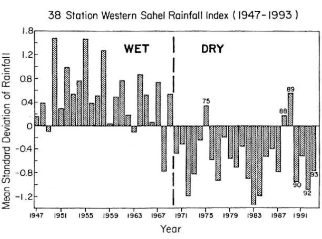
Figure 1.4 Mean standard deviations of rainfall for the 38-station June-September western Sahelian index. The boldface line indicates the least-squares best fit line to the data. Data presented are from 1949 to 1990. Figure from Landsea and Gray (1992).. . . 11

Figure 1.5 Solution for heating symmetric about the equator in a shallow-water model. (top) Contours of vertical velocity w (positive w solid; negative w dashed) super-imposed on the velocity field (vectors) for the lower layer. The field is dominated by the upward motion in the heating region where it has approximately the same shape as the heating function. Elsewhere there is subsidence with the same pattern as the pressure field. (bottom) Contours of pressure purturbation p in the lower layer which is negative everywhere. Two cyclones are found on the northwest and southwest flanks of the forcing region. Image from Gill (1980). . . 12

Figure 1.6 Idealized portrayal of upper level wind patterns during wet (upper panel) versus dry (lower panel) Western Sahel years. Image from Landsea and Gray (1992). 13

(9)

simulated by the GFDL (solid line) and MIROC (dashed line) models. Anomalies are in mm day−1_{. Image from Biasutti et al. (2008). . . 14}

Figure 2.1 Carbon emission scenarios from the Special Report on Emissions Scenarios (SRES) for the International Panel on Climate Change’s Fourth Assessment Report (IPCC-AR4). Carbon concentrations are expressed in parts per million (ppm). . . 18

Figure 2.2 Domains used in this study. Also shown are the locations of all tropical cyclones during the months of July through October 1958-2003 when they were first named. Image from Aiyyer and Thorncroft (2006). . . 19

Figure 3.1 Annual cycle of Ni˜no-3 SST (degrees K) in observations (Kaplan dataset, solid black line) and in model simulations of the 20th century (20C3M simulation, red dashed line) and 21st century (A1B simulation, blue dashed line). . . 39

Figure 3.2 Wavelet and spectral analysis of Ni˜no-3 SST for the Hadley SST dataset (top left) and 21 IPCC GCMs. . . 42

Figure 3.3 Plots of correlation (shaded) and regression (vectors, ms−1

) of JAS shear and the Ni˜no-3 index. . . 45

Figure 3.4 Annual cycle of Sahel rainfall (mm month−1

) in observations (Hulme dataset, solid black line) and in model simulations of the 20th century (20C3M simulation, red dashed line) and 21st century (A1B simulation, blue dashed line). . 48

Figure 3.5 Wavelet and spectral analysis of Sahel precipitation for the Hulme precip-itation dataset (top left) and 21 IPCC GCMs.. . . 51

Figure 3.6 Plots of correlation (shaded) and regression (vectors, ms−1_{) of JAS shear}

and the Sahel index. . . 54

Figure 3.7 Idealized illustration showing two circular wind gyres (vectors) and their corresponding streamfunction fields (contours). H stands for high pressure and L stands for low pressure. Winds around the left gyre are rotating in a clockwise sense and are represented by circular streamfunction contours that are increasing towards the center. Winds around the right gyre are rotating in a counterclockwise sense and are represented by circular streamfunction contours that are decreasing towards the center. . . 57

Figure 3.8 Streamfunction (contour interval 2.5 X 10−6

m2

s−1

(10)

Figure 3.9 Velocity potential (contour interval 1.0 X 10−6

m2

s−1

) and irrotational wind (vectors) at 200 hPa for July-September 1948-1999 for the NCEP/NCAR reanalysis (top left) and 20C3M model simulations. Positive velocity potential depicted by blue solid contours; negative velocity potential depicted by red dashed contours. . . 61

Figure 4.1 IPCC-AR4 multi-model projections of June-November vertical wind shear change. (a) The 18-model ensemble-mean change in June-November 850-200 hPa vertical wind shear (shaded, m s−1 ◦ _C−1 _{warming), contours show ensemble-mean}

background shear (2001-2020 average, m s−1_{); (b) Number of models (out of 18)}

showing positive change in shear. Box indicates the MDR. Figure from Vecchi and Soden (2007). . . 74

Figure 4.2 IPCC-AR4 multi-model projections of July-September vertical wind shear change. Number of models (out of 21) showing an (a) increase, (b) decrease, and (c) no significant change in 850 hPa-200 hPa shear (m s−1_{). Significance determined}

at the 95% confidence level using the Student’s t-test. Dots indicate locations of tropical cyclone genesis over the period 1948-2004; box indicates a region of frequent tropical cyclone development (MDR). . . 75

Figure 4.3 IPCC-AR4 multi-model projections of July-September vertical wind shear change. Number of models (out of 21) showing an increase, decrease, and no change in three sections of the MDR. Trends averaged for all gridpoints throughout each section. . . 76

Figure 4.4 Same as in Figure 4.2, but for precipitation (kgm−2

s−1

). Box indicates Sahel region in West Africa. . . 77

Figure 4.5 Linear correlations between the IPCC-AR4 model projections of July-September vertical wind shear timeseries versus the Sahel rainfall timeseries before (blue bars) and after (red bars) linearly regressing the ENSO timeseries out of the MDR shear data. . . 78

Figure 4.6 IPCC-AR4 multi-model projections of July-September Sahel rainfall anoma-lies versues 850 hPa-200 hPa vertical wind shear anomaanoma-lies. Each dot represents a model-projected JAS seasonal anomaly of Sahel rainfall versus MDR shear. Linear regression plotted as red line; percentage of seasonal anomalies in each quadrant given in corners of plot. . . 79

Figure 4.7 IPCC-AR4 model projections of July-September vertical wind shear changes in the MDR (red lines) and Sahel rainfall changes (blue lines). Trends are normalized to the mean. . . 80

(11)

versus 850 hPa-200 hPa vertical wind shear change in the (a) western MDR, (b) central MDR, and (c) eastern MDR. Each dot represents one model in the ensemble. Linear regression plotted as red line. . . 81

Figure 4.9 Same as Figure 4.2, but for the GFDL-20, GFDL-21, HADCM, MIROC-HI, and INGV models only. . . 82

Figure 4.10 Same as Figure 4.4, but for the GFDL-20, GFDL-21, HADCM, MIROC-HI, and INGV models only. . . 83

(12)

List of Tables

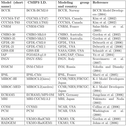
Table 2.1 List of the models used in this study. . . 20

Table 2.2 Atmospheric and oceanic resolutions of the models used in this study (in degrees). . . 21

Table 3.1 Calculated skewness and kurtosis values of JAS Ni˜no-3 SST for 20th century observations (Hadley SST) and the 20th and 21st century simulations of 21 IPCC AR4 GCMs. Kurtosis values are calculated by subtracting the kurtosis of the normal distribution (kurtosis = 3) to obtain a kurtosis relative to the normal distribution. 64

Table 3.2 Calculated skewness and kurtosis values of Sahel precipitation for 20th cen-tury observations (Hulme precipitation) and the 20th and 21st cencen-tury simulations of 21 IPCC AR4 GCMs. Kurtosis values are calculated by subtracting the kurtosis of the normal distribution (kurtosis = 3) to obtain a kurtosis relative to the normal distribution. . . 65

(13)

Chapter 1

Introduction

1.1 Motivation

The concentration of greenhouse gases in the atmosphere, particularly carbon

diox-ide, has been increasing since the onset of the industrial revolution in the late 18th and early

19th centuries (IPCC 2001). Through the well-understood process of absorbing terrestrial

radiation emitted by the Earth and transmitting it back to the surface as longwave

radia-tion, greenhouse gases like carbon dioxide act to increase the global-mean tropospheric air

temperature.

The Third Assessment Report of the United Nations Intergovernmental Panel

on Climate Change (IPCC-AR3) concluded that most of the observed warming in recent

decades is likely due to a rapid increase in anthropogenic greenhouse gas concentrations.

Furthermore, the IPCC’s Fourth Assessment Report (IPCC-AR4) suggests that the

warm-ing associated with increased greenhouse gas concentrations has penetrated into the global

oceans in the past 40 years, supported by an observed 0.25 - 0.5 degree C increase in SST

over most tropical ocean basins (Webster et al. 2005).

Tropical cyclones (TCs) are one of the most destructive natural phenomena and

impact a significant portion of the world’s population (e.g. Pielke and Landsea 1998). A

major problem, that has been well recognized, is the potential for increased vulnerability

of coastal areas in a warmer climate. Scientists have debated the implications of climate

(14)

through the transfer of latent and sensible heat from the oceans, an initial concern is

that increased sea surface temperature (SST) due to anthropogenic forcing will lead to

more frequent and intense hurricanes (Houghton et al. 1990). However, SST is only one

factor in the development and intensification of tropical cyclones, and the numerous other

thermodynamical and dynamical processes that govern tropical cyclone activity cannot

be overlooked. These processes vary on interannual to multidecadal timescales, and the

variability of tropical cyclone genesis frequency is driven in part by the spatio-temporal

variability of these environmental factors.

Among these factors, vertical wind shear is a key environmental variable that

exerts a direct influence on seasonal tropical cyclone activity. On interannual time scales,

vertical wind shear explains 30 to 50% of the variability of tropical cyclones within the main

development region (MDR) of the tropical North Atlantic, the area where the majority of

Atlantic tropical cyclones form (Aiyyer and Thorncroft 2006). Tropical cyclones in all basins

historically tend to form where shear is low, as depicted in Figure 1.1.

It is well understood that the presence of substantial (at least 10ms−1

) deep-layer

vertical wind shear in the background environment has a detrimental effect on the genesis

and intensification of tropical cyclones by inhibiting the organization of convection needed

to maintain tropical cyclones (e.g. Ramage 1959). Figure 1.2 shows how in a heavily sheared

environment, convection is displaced from the center of the storm, leaving the center of

low-level circulation exposed. The physical mechanism for the effect of shear on tropical cyclones

is usually understood in terms of ’ventilation’, where differences in upper- and lower-level

flow advect heat and moisture away from the system, effectively inhibiting intensification

of the disturbance (Gray 1968). An alternate explanation given by DeMaria (1996) is one

of ’tilting and stabilization’ in which shear causes potential vorticity (PV) associated with

the circulation to become tilted in the vertical. This induces mid-level warming near the

center of the vortex, which acts to reduce convective activity and inhibit intensification.

Simulations from a suite of fully-coupled global climate models collected for the

International Panel on Climate Change’s Fourth Assessment Report (IPCC-AR4) provide

an unparalleled opportunity to explore the effects of climate change on tropical cyclone

activity. To fully understand the model-predicted changes in vertical wind shear in the

(15)

tropical Atlantic. This study takes a statistical approach to investigate whether predictions

in vertical wind shear trends over the MDR are related to model projections for future

rainfall trends in the Sahel. We examine trends and correlations between summertime Sahel

rainfall and vertical wind shear in the MDR over the 21st century. It is hypothesized that

the spread in projections of future Sahel rainfall variability contributes to the uncertainty

in MDR shear predictions.

1.2 Climatic Forcings Modulating Atlantic Vertical Wind Shear

Variability of vertical wind shear in the MDR is influenced by changes in the

large-scale background circulation, forced by teleconnections such as the El Ni˜no-Southern

Oscillation (ENSO) and the West African monsoon system (e.g. Landsea and Gray 1992;

Goldenberg and Shapiro 1996; Aiyyer and Thorncroft 2006). These teleconnections directly

impact the vertical wind shear over the MDR through alterations of the upper-level flow in

the tropical Atlantic basin on interannual to multidecadal timescales.

While the interannual variability of shear is better understood, the absence of

ac-curate observational datasets before the mid 20th century greatly limits our understanding

of fluctuations on longer timescales. In the first half of the 20th century, we relied on

mili-tary aircraft reconnaissance and land and ship observations to detect and observe tropical

cyclones. Observations were random and spotty, thus the accuracy of early observational

datasets is called into doubt (Landsea 1993; Landsea et al. 1999). However, the revolution

of satellite technology in the 1960’s has greatly improved our understanding of tropical

cy-clone activity. Despite the relatively short period of reliable TC records, we are coming to a

better understanding of the processes that influence vertical wind shear, and subsequently,

tropical cyclones in the tropical Atlantic basin. This section details some of these processes.

1.2.1 West African rainfall

The Sahel region of West Africa is a semi-arid transitional zone, bounded to the

north by the Sahara Desert and to the south by rainforests that flourish from the humid

equatorial tropical climate. The Sahel experiences rather extreme decadal fluctuations in

(16)

debated to this day. Some argue that this can be explained by land surface use (e.g.

deforestation) and its feedback on atmospheric radiation and precipitation (Charney et al.

1977), while others believe that Sahel rainfall variability is governed by fluctuations in

global sea surface temperatures (Palmer 1986; Folland et al. 1986). The latter theory is

currently favored to be the main cause of 20th century Sahel rainfall variability thanks

to recent modeling studies employing coupled GCMs (e.g. Giannini et al. 2003; Lu and

Delworth 2005; Hoerling et al. 2006), while changes in vegetation and land surface likely

act to amplify Sahel precipitation anomalies (e.g. Zeng and Neelin 2000).

A strong multidecadal relationship between West African rainfall and Atlantic

hur-ricane activity is evident in the 20th century observational dataset (e.g. Gray 1990; Landsea

and Gray 1992). For example, there were significantly fewer Atlantic major hurricanes

dur-ing the period 1947 to 1969 which coincided with a severe drought in the Sahel region, and a

marked uptick in Atlantic major hurricane frequency between 1970 to 1987 when the Sahel

region experienced plentiful rainfall. This is particularly evident when comparing the

num-ber of tropical cyclone tracks between the two 24-year periods of 1944-1967 (relatively wet

Sahel period) and 1968-1991 (relatively dry Sahel period) in Figure 1.3. Note the drastic

shift from wet to dry conditions in the Sahel in the late 1960’s in Figure 1.4, one example

how the Sahel region experiences large swings in precipitation over decadal timescales.

One physical mechanism in which Sahel rainfall relates to tropical cyclone activity

in the Atlantic is through the modification of vertical wind shear in the main development

region (MDR) of the tropical Atlantic, a region where tropical cyclone development is

climatologically favored. The Sahel-MDR shear relationship can be understood in terms of

the tropical atmospheric response to steady monsoonal thermal forcing as in the

Matsuno-Webster-Gill mechanism. Upper-level anticyclonic gyres to the west of the Sahel monsoon

region represent the stationary Rossby wave driven by persistent diabatic thermal forcing

(Gill 1980). This is illustrated in Figure 1.5 but for the lower levels where cyclonic gyres

result to the west of the forcing. The net effect is anomalous upper-level easterly flow

over the central and eastern MDR in conjunction with a wetter Sahel, which acts to cancel

some of the climatological upper-level westerly flow and reduce vertical wind shear in those

regions. Figure 1.6 shows an idealization of the differences in flow in the tropical Atlantic

(17)

As depicted in previous studies (e.g. Held et al. 2005; Biasutti et al. 2008;

Cook and Vizy 2006), the outlook for Sahel rainfall in a warming climate as depicted by

global climate models is very uncertain. Figure 1.7 puts this in perspective, showing how

two GCMs from the IPCC-AR4 archive (the GFDL and MIROC models) produce widely

varying solutions for 21st century Sahel rainfall. This is surprising given that the very same

models were robust in replicating 20th century precipitation patterns in the Sahel when

forced with historic time series of sea surface temperatures (Giannini et al. 2003; Tippett

and Giannini 2006; Lu and Delworth 2005; Hoerling et al. 2006).

1.2.2 El Ni˜no-Southern Oscillation

The El Ni˜no-Southern Oscillation is the largest system of climate variability in the

world, influencing global weather on interannual to multidecadal timescales. The theoretical

framework of ENSO can be understood through the work of Bjerknes (1966) who described

the positive feedback loop that drives ENSO in the tropical Pacific Ocean. Wind anomalies

in the central equatorial Pacific generate thermocline anomalies which travel to the east

towards the coasts of Peru and Chile. In the eastern equatorial Pacific these upwell as

warm SST anomalies, which in turn give rise of wind anomalies in the central Pacific.

Later work by Wyrtki (1975) and Picaut et al. (1996) describe a secondary feedback loop

in the central Pacific whereby SST is affected directly by wind anomalies via advection,

anomalous upwelling, evaporation, and mixed-layer depth anomalies. These SST anomalies

in turn influence the wind.

The work of Gray (1984) documents how ENSO serves as a teleconnection for

vertical wind shear in the tropical Atlantic. During the El Ni˜no phase of ENSO, warmer

than average SSTs in the eastern Pacific shift convective activity to the east. This in

turn leads to westerly upper-level wind anomalies over the tropical Atlantic, which acts to

strengthen the climatological westerly upper-level flow in the Atlantic. Vertical wind shear

in the Atlantic is thus enhanced during El Ni˜no years. During La Ni˜na years, convection

over the eastern Pacific is suppressed due to cooler than average SSTs. Thus, the westerly

upper-level flow over the tropical Atlantic is comparatively weaker, and shear is reduced.

As evident in many observational datasets, the El Nino-Southern Oscillation

(18)

ability (or lack thereof) of coupled global climate models (GCMs) to simulate ENSO’s

vari-ability has been the focus of recent studies (e.g. van Oldenborgh et al. 2005; Lin 2007a).

Using wavelet analysis, Lin (2007a) compared 20th century observational datasets to the

20th century output from the suite of IPCC GCMs and found that the models display a

wide range of skill in simulating the interdecadal variability in ENSO’s amplitude and

pe-riod. The suite of models can be broken into three groups according to whether the model

has a pronounced spectral peak shorter than, greater than, or similar to that of the 20th

century observations. It was found that 8 of the 21 models in the IPCC-AR4 archive

dis-play significant interdecadal variability of ENSO in both amplitude and period (Lin 2007a).

Furthermore, Lin (2007a)a concludes that only one model (MPI) is able to reproduce the

observed eastward shift of the westerly anomalies in the low-frequency regime of ENSO.

It is of interest to examine how and if the spatio-temporal variability of ENSO

changes under projected global warming conditions in the 21st century. van Oldenborgh

et al. (2005) selects six models in the IPCC archive that seem to best simulate ENSO in

the 20th century and then analyzes output from the years 2051-2100 under various global

warming scenarios (but mainly the A2 scenario). By analyzing projected changes in the

mean state, amplitude, and skewness (a comparison of the magnitude of anomalies between

El Ni˜no and La Ni˜na phases), their study finds that these six most realistic models show no

statistically significant changes in the spatial structure or temporal variations in ENSO in

the latter half of the 21st century. Thus, they conclude that there is very little evidence from

the IPCC models that support a major change in the ENSO phenomenon in the 21st century

under global warming conditions. Additionally, Collins and the CMIP Modeling Groups

(2005) finds that GCMs show no trend in the mean state of ENSO towards more El Ni˜

no-like or La Ni˜na-like conditions when forced with 80 years of the 1% per year CO2 increase

scenario.

1.3 Objectives

Simulations from a suite of fully-coupled global climate models collected for the

International Panel on Climate Change’s Fourth Assessment Report (IPCC-AR4) provide

(19)

To fully understand the model-predicted changes in vertical wind shear in the MDR, we

must examine the numerous mechanisms that influence circulation patterns in the tropical

Atlantic. This study takes a statistical approach to investigate whether model predictions

in vertical wind shear trends over the MDR is related to model projections for future rainfall

trends in the Sahel. We examine trends and correlations between summertime Sahel rainfall

and vertical wind shear in the MDR over the 21st century. It is suggested that the spread in

projections of future Sahel rainfall variability contributes to the uncertainty in MDR shear

predictions.

Our goal is to address the following questions:

• Which (if any) GCMs in the IPCC-AR4 archive are able to accurately replicate

well-known features of the 20th century climate like ENSO and the West African monsoonal

system so that those models can be used to form conclusions about changes to our

climate in the 21st century?

• Do the best models exhibit a consistent MDR shear trend in the 21st century?

• Does the spread in projections of future Sahel rainfall variability contribute to the

uncertainty in MDR shear projections in the 21st century?

In the following chapter a description of data and methods used to study these

questions will be presented. First, spatio-temporal characteristics for the West African

monsoon and ENSO cycle for the entire 21-member IPCC model suite will be analyzed.

Based on model performace in simulating the familiar patterns associated with the ENSO

cycle and West African monsoon, each model will be assigned a confidence level for the

reliability of their 20th century predictions. Next, a statistical approach will be used to

gauge the relative roles of various teleconnections in modulating vertical wind shear in the

tropical Atlantic under 21st century warming conditions. Results will be presented for the

full suite of models, as well as the group of models selected from the previous chapter for

their reliable simulations of the 20th century climate. Last, all findings will be summarized,

(20)

(21)

(22)

(23)

(24)

(25)

(26)

(27)

Chapter 2

Data and Methodology

2.1 Data

This study utilizes gridded monthly-averaged data from a 21-member suite of

fully-coupled ocean-atmosphere global climate models collected for the Intergovernmental

Panel on Climate Change 4th Assessment Report (IPCC-AR4). The model outputs, made

available by various modeling groups around the world, were extracted from the Program

for Climate Model Diagnosis and Intercomparison (PCMDI) website. See Tables 2.1 and

2.2 for a complete list of the models used in this study, along with their atmospheric and

oceanic resolutions. It should be noted that there is a wide range in atmospheric and oceanic

resolutions across the suite of models. Multiple simulations for the same period for each

model are available, but for the sake of simplicity, only the first simulation (run1) of each

model is used here. A handful of models from the IPCC archive (GISS-AOM, GISS-ER,

MIUB-ECHO) were omitted from this study due to data availability and processing issues

at the time of publication, but the exclusion of these models should not affect the outcome

of this study. It is hopeful that the models selected for this study are representative of the

multi-model ensemble provided for the IPCC.

Two different model simulations are used: the 20C3M simulation for the 20th

century and the SRES-A1B scenario for the 21st century. The 20C3M simulations are

the best efforts of the modeling groups to simulate the climate of the 20th century using

(28)

emission scenarios from the Special Report on Emissions Scenarios (SRES) prepared by

the IPCC for the Third Assessment Report (IPCC-AR3) in 2001. Because climate change

depends heavily on human activity, the climate models must be forced with future scenarios

of greenhouse gas (e.g. carbon dioxide, aerosols) concentrations to make predictions of

what lies ahead in terms of climate change. The A1B scenario assumes a future world of

extensive economic growth, rapid development of new and more efficient technologies, and

a global population that peaks around 2050 and declines afterwards. In the A1B scenario,

concentrations of emissions experience a steep increase in the first few decades of the 21st

century before leveling off around the year 2050 and declining thereafter. It is assumed to

be a ’middle-of-the-road’ approach to climate change, assuming that there will be moderate

progress in the 21st century to curb greenhouse gas emissions. The A1B scenario was

chosen over the other available scenarios because it appears to be the most widely accepted

scenario across literature dealing with climate change based on a review of past studies. See

Figure 2.1 for a comparison of the different SRES scenarios in terms of their greenhouse gas

forcings.

To characterize the present climate and to validate model simulations for the 20th

century, we employ several monthly-averaged observational datasets. The Hulme

observa-tional dataset (Hulme 1992), covering the years 1900-1998 with a resolution of 2.5◦ _latitude

by 3.75◦ _{longitude, is used to obtain historial precipitation totals from the Sahel region}

of West Africa. Historial sea surface temperatures for the Nino3 region in the Pacific are

obtained from the Met Office Hadley Centre’s Sea Ice and SST (HADISST) (Rayner et al.

2003), covering the years 1890-1999 with a resolution of 1◦ _{latitude by 1}◦ _{longitude. Wind}

data are from the NCEP/NCAR reanalysis (Kalnay et al. 1996), spanning 1948-1999 on a

2.5◦ _{x 2.5}◦ _{global grid.}

2.2 Domains

Figure 2.2 highlights the domains used in this study. The domains are as follows:

the MDR (7.5◦_-20◦_{N, 80}◦_-20◦_{N); the Sahel region (10}◦_-20◦_{N, 20}◦_-20◦_{E); and the Ni˜}

no-3 region (5◦_N-5◦_{S, 150}◦_-90◦_{W). The Ni˜}_{no-3 region is used to represent SST fluctuation}

(29)

summertime monsoonal precipitation. The MDR is a section of the tropical North Atlantic

that is climatologically favored for tropical cyclone development.

2.3 Methods

To capture the climatological peak of the Atlantic hurricane season, we use

July-September (JAS) mean data over the respective region for each year. Vertical wind shear

in the MDR is defined as the vector difference between the winds at 850 hPa and 200 hPa,

consistent with previous literature. Both the zonal and meridional components of the wind

field are used to derive the shear vector for each month, and each component of the total

wind shear vector is examined to see their individual contribution to the total wind shear

(30)

(31)

(32)

Table 2.1: List of the models used in this study.

Model (short name)

CMIP3 I.D. Modeling group and country

Reference

BCCR BCCR-BCM2.0 BCCR, Norway BCCR Model

Develop-ers (2004)

CCCMA-T47 CGCM3.1(T47) CCCMA, Canada Kim et al. (2002) CCCMA-T63 CGCM3.1(T63) CCCMA, Canada Kim et al. (2002)

CNRM CNRM-CM3 CNRM, France Salas-Melia et al.

(2005)

CSIRO-30 CSIRO-Mk3.0 CSIRO, Australia Gordon et al. (2002) CSIRO-35 CSIRO-Mk3.5 CSIRO, Australia Gordon et al. (2002)

GFDL-20 GFDL-CM2.0 GFDL, USA Delworth et al. (2006)

GFDL-21 GFDL-CM2.1 GFDL, USA Delworth et al. (2006)

GISS-EH GISS-EH NASA/GISS, USA Schmidt et al. (2006)

IAP FGOALS-g1.0 LASG/IAP, China Yu et al. (2004)

INGV INGV-SXG INGV, Italy Scoccimarro et al.

(2007)

INMCM INM-CM3.0 INM, Russia Volodin and Diansky

(2004)

IPSL IPSL-CM4 IPSL, France Marti et al. (2005)

MIROC-HI MIROC3.2(hires) CCSR/NIES/FRCGC, Japan

K-1 Model Developers (2004)

MIROC-MED MIROC3.2(medres) CCSR/NIES/FRCGC, Japan

K-1 Model Developers (2004)

ECHAM5 ECHAM5/MPI-OM MPI, Germany Jungclaus et al. (2006)

MRI MRI-CGCM2.3.2 MRI, Japan Yukimoto and Noda

(2002)

CCSM CCSM3 NCAR, USA Collins et al. (2006)

PCM PCM NCAR, USA Washington et al.

(2000)

HADCM UKMO-HadCM3 UKMO, UK Gordon et al. (2000)

(33)

Table 2.2: Atmospheric and oceanic resolutions of the models used in this study (in degrees).

Model Atmos. resolution Ocean resolution BCCR 2.81◦ _{x 2.79}◦ _0.5-1.5◦ _{x 1.5}◦

CCCMA-T47 3.75◦ _{x 3.71}◦ _1.85◦ _{x 1.85}◦

CCCMA-T63 2.81◦ _{x 2.79}◦ _1.4◦ _{x 0.9}◦

CNRM 2.81◦ _{x 2.79}◦ ₂◦ _{x 0.5}◦

CSIRO-30 1.88◦ _{x 1.87}◦ _1.88◦ _{x 0.84}◦

CSIRO-35 1.88◦ _{x 1.87}◦ _1.88◦ _{x 0.84}◦

GFDL-20 2.5◦ _{x 2}◦ ₁◦ _{x 1/3}◦

GFDL-21 2.5◦ _{x 2}◦ ₁◦ _{x 1/3}◦

GISS-EH 5◦ _{x 4}◦ ₂◦ _{x 2}◦

IAP 2.81◦ _{x 3.05}◦ ₁◦ _{x 1}◦

INGV 1.125◦ _{x 1.125}◦ ₂◦ _{x 1}◦

INMCM 5◦ _{x 4}◦ _2.5◦ _{x 2}◦

IPSL 3.75◦ _{x 2.54}◦ ₂◦ _{x 1}◦

MIROC-HI 1.13◦ _{x 1.12}◦ _0.28◦ _{x 0.19}◦

MIROC-MED 2.81◦ _{x 2.79}◦ _1.4◦ _{x 0.5}◦

ECHAM5 1.88◦ _{x 1.87}◦ _1.5◦ _{x 1.5}◦

MRI 2.81◦ _{x 2.79}◦ _2.5◦ _{x 0.5}◦

CCSM 1.41◦ _{x 1.4}◦ _1.13◦ _{x 0.27}◦

PCM 2.81◦ _{x 2.79}◦ _1.13◦ _{x 0.27}◦

HADCM 3.75◦ _{x 2.5}◦ _1.25◦ _{x 1.25}◦

(34)

Chapter 3

Model Validation

3.1 Introduction

In this chapter, various properties of 20th century simulations of ENSO, Sahel

precipitation, and 200-850 hPa wind fields will be examined for the 21-member suite of

IPCC GCMs selected for this study. Understanding individual model behavior and biases

is important before using the model outputs to make any predictions about the future

climate. This is especially important given the rather coarse resolution of these GCMs

which could possibly hinder model performance on simulating the variability of various

atmospheric and oceanic phenomena, such as the West African monsoon.

Are the current GCMs ready to be used to make predictions about changes in

tropical Atlantic vertical wind shear and its associated teleconnections in a future climate?

The goal of this section is to identify and analyze the wide range of behavior exhibited

across the suite of models, and then select the models that produce realistic simulations of

the 20th century climate to make predictions about the future climate in the next chapter.

3.2 El Nino-Southern Oscillation

3.2.1 Annual Cycle

We begin our analysis by comparing the annual cycle of SST variations in the

(35)

monthly SST in the Ni˜no-3 region for the 20th century (20C3M; dashed red line) and 21st

century (A1B; dashed blue line) simulations for each of the models. The modeled annual

cycles are plotted against years 1901-1999 of the Hadley SST dataset (solid black line) to

compare and contrast model performance.

Observations show a peak in eastern Pacific SSTs in the spring months (maximum

in April) and a gradual decrease in SST through the summer months beforing bottoming

out in the late summer to fall months. There is an approximately 2.5 degree Kelvin seasonal

difference between the peak in the spring and the minimum in the fall. The models have

a wide range of skill in capturing this pattern of seasonal variability in the 20th century

simulations. IAP is nearly devoid of any seasonal fluctuation of SST in the eastern Pacific.

Several models (e.g. BCCR, INMCM, ECHAM5) delay the springtime peak in SST to

varying degrees. Other models depict more than one distinct SST peak throughout the

year (GISS-EH, PCM). GISS-EH has a primary peak in March and a secondary peak in

October, while PCM has two peaks of roughly the same magnitude in June and December.

It also appears that a large number of the models have a cold bias throughout the year when

compared to the observations, which in some cases is rather drastic (e.g. BCCR, INGV).

Lin (2007b) attributes this cold bias to the ’double ITCZ’ problem that plagues many of the

GCMs, where excessive precipitation over much of the tropics causes stronger than normal

trade winds, excessive SST-surface latent heat flux, and insufficient SST-surface shortwave

flux. This results in a mean cold bias across much of the tropical ocean basins in the GCMs.

Overall, only a handful of models (both GFDL models, both MIROC models, MRI, and

HADCM) have reasonable simulations of the observed seasonal cycle of SST in the East

Pacific.

3.2.2 Statistical Analysis of Observations vs. Model Simulations

Hoerling et al. (2001) concluded that the tropical and extratropical atmospheric

response to opposite phases of ENSO is nonlinear. In other words, El Ni˜no and La Ni˜na

events of equal magnitudes do not have an equal effect on the upper tropospheric flow over

the tropical Atlantic. Thus, it is important for GCMs to simulate the correct number and

distribution of warm vs. cold events in the eastern Pacific to ensure that their atmospheric

(36)

matter.

There are several statistical measures that are useful for gauging the relative

mag-nitude and quantity of warm vs. cold ENSO events in the eastern Pacific as simulated by

the GCMs. Skewness is a statistical measure that gauges the asymmetry of the distribution

of a dataset. A normal distribution, or one that is perfectly symmetric about the mean, has

a skewness of zero. For unimodal distributions, positive skewness indicates that the ’tail’

of the distribution is more stretched on the positive side of the mean. Negative skewness

indicates that the tail is more stretched below the mean. Kurtosis, on the other hand,

measures the normality of a distribution. A normal distribution, or one whose distribution

is bell-shaped and peaked at the mean, has a kurtosis of 3. We subtract this value from the

calculated kurtosis to give us values that are relative to the normal distribution. Positive

values of kurtosis indicate that the distribution is more sharply peaked than the normal

distribution (leptokurtic), and negative values result from a distribution that is ’flatter’

than the normal distribution (platykurtic).

3.2.3 Observed vs. Simulated ENSO Skewness and Kurtosis

The skewness and kurtosis of the detrended 20th century (years 1901-1999) JAS

seasonal mean Ni˜no-3 timeseries from the Hadley SST dataset is calculated. The calculated

skewness from the observations is 0.64, meaning that SST anomalies in the Ni˜no-3 region

are generally larger during El Ni˜no years than La Ni˜na years. This result is consistent with

van Oldenborgh et al. (2005), where a skewness of 0.54 was determined from the Kaplan

SST dataset using an EOF analysis. van Oldenborgh et al. (2005) did not calculate kurtosis,

so from the Hadley SST dataset we determine that the Ni˜no-3 kurtosis for the 20th century

is 0.61. A leptokurtic kurtosis such as this indicates that the distribution of seasonal means

in the 20th century is relatively sharply peaked.

Skewness and kurtosis calculations are then repeated for the detrended 1901-1999

JAS Ni˜no-3 timeseries for each of the 20th century (20C3M) IPCC GCM simulations. The

resulting values for each model are listed in Table 3.1. As a whole, the models do not produce

a realistic asymmetry of positive El Ni˜no vs. negative La Ni˜na events in the simulations, as

evident from the negative values of skewness that are returned by several GCMs. Eight out

(37)

CCSM, HADGEM) display a negative skewness, meaning that SST anomalies are generally

larger during La Ni˜na years rather than El Ni˜no years. This is uncharacteristic of the 20th

century observations, which exhibit a large positive skewness. Only three models

(GFDL-21, MIROC-HI, and HADCM) produce realistic positive skewnesses (0.67, 0.38, and 0.58,

respectively). The remaining 10 models (CNRM, CSIRO-35, GFDL-20, GISS-EH, IAP,

INGV, INMCM, ECHAM5, MRI, and PCM) have weakly positive skewnesses.

Kurtosis values for the 20th century Ni˜no-3 model simulations are then calculated

and analyzed. The models exhibit a diverse variety of distributions evident from the wide

range of calculated kurtosis. For example, the nature of the distributions ranges from very

platikurtic with the IAP model (relative kurtosis of -1.35) to relatively sharply peaked

with the CCCMA-T63 model (relative kurtosis of 0.91). The three models that have the

most realistic 20th century skewnesses from the previous section (GFDL-21, MIROC-HI,

HADCM) also have leptokurtic distributions, consistent with observations.

For completeness, the raw observed timeseries and the simulated timeseries are

correlated for each model (not shown). The two timeseries are not very well correlated at

all, with some models even being anticorrelated with the observations. This is not surprising,

given that is unlikely for individual El Ni˜no or La Ni˜na events in the observations to correlate

with those from a free-running climate model.

Thus, we can conclude from our statistical analysis of Ni˜no-3 skewness and kurtosis

that only three models (GFDL-21, MIROC-HI, and HADCM) have realistic distributions

of simulated seasonal mean JAS Ni˜no-3 SST compared to the 20th century observations

from the Hadley SST dataset. The distributions of seasonal averages for each of these

models are asymmetric, skewed towards positive (El Ni˜no) anomalies, and are leptokurtic,

consistent with the 20th century observed climate. These three models have been assigned

a higher confidence level for their 20th century simulations. Several other models have poor

statistical representation of ENSO variability and thus have been assigned lower confidence

levels.

3.2.4 ENSO Wavelet and Spectral Analysis

As evident in many observational datasets, the El Ni˜no-Southern Oscillation

(38)

Here we utilize wavelet and spectral analyses to compare and contrast the modeled ENSO

variability in the 20th century simulations with observations. Spectral analysis allows us

to determine the prominent peaks of variability over a given period of time. An even more

useful tool is wavelet analysis where we can not only determine different peaks of variability,

but also see how the different modes of variability change with time (Torrence and Compo

1998).

The Hadley SST observational dataset depicts a wide range of interdecadal

vari-ability in Ni˜no-3 SST (Figure 3.2). Spectral analysis reveals a rather broad peak between

2-6 years, with the highest peak around 3 years. Wavelet analysis shows that most of the

variability is concentrated before 1920 and after 1950, with a relative lull in amplitude

between the years 1920-1950. From 1900-1950, the dominant period fluctuates greatly

be-tween 2-8 years. Bebe-tween 1950-1960, longer timescales dominate with a period bebe-tween 5-7

years. After 1960 until the end of the 20th century, there is a marked shift towards shorter

periods (2-5 years).

Next, spectral and wavelet analyses are performed on the model simulations of

the 20th century in Figure 3.2. We are looking for models that have realistic simulations

of ENSO variability, i.e., models whose variability differs in both amplitude and period

throughout the 20th century. It is evident that the models have a wide range in skill in

simulating the interdecadal variability of ENSO observed in the 20th century, consistent

with Lin (2007a). Some models (IAP, CNRM) have constant amplitude and near-biennial

ENSO oscillations throughout the entire course of the 20th century, which is quite

unre-alistic. Yu et al. (2004) determined that the cause of the very strong and regular ENSO

oscillations in the IAP model is due to the ’double ITCZ’ problem in GCMs where cold

biases in the tropical Pacific are amplified through the air-sea coupling in the models. Other

models have spectral peaks that are significantly shorter (e.g. CCSM, GFDL-20) or longer

(e.g. CCCMA-T63, MIROC-MED) than the observations. However, it is encouraging to see

that a number of models (e.g. BCCR, GFDL-21, HADCM, HADGEM, ECHAM5, INGV,

MIROC-HI) simulate the interdecadal variability of ENSO to some degree, in both

ampli-tude and period. Take for example the BCCR model, which has significant episodes of 3-6

year variability between 1900-1920, 5-7 year variability between 1940-1950, and 2-5 year

(39)

3.2.5 Shear-ENSO Regression and Correlation

In this section we use plots of linear correlation and regression to analyze the

spatial relationship between Ni˜no-3 SST and JAS shear. The regression analysis is useful

for determining the pattern of anomalous shear that arises from warm SST episodes in

the eastern Pacific. Figure 3.3 shows correlations and regression between JAS vertical

wind shear and the Ni˜no-3 index in the 20th century observations and the model 20C3M

simulations. Historical wind data are obtained from the NCEP/NCAR reanalysis and SST

data are from the Hadley SST dataset. The observations reveal a broad swath of regressed

westerlies and generally positive correlations across much of the MDR. The anomalous

westerly shear over the MDR is in response to enhanced convective activity from warm

events (El Ni˜no) in the eastern Pacific. The direct relationship between Ni˜no-3 SST and

shear over the tropical Atlantic is highlighted by the zonally elongated strip of positive

correlation across the MDR. This westerly shear is most pronounced in the Carribean

western MDR which is closer to the SST forcing. Thus, we can see that increased westerly

shear in the MDR is associated with anomalously warm SST in the eastern Pacific, consistent

with Goldenberg and Shapiro (1996) and Aiyyer and Thorncroft (2006).

GISS-EH and HADGEM show very little relationship between shear and ENSO

across the tropical Atlantic. These two models have no distinct pattern of significant

cor-relations in the MDR (MDR-averaged shear-ENSO correlation values of -0.16 and 0.15 for

GISS-EH and HADCM, respectively), and there is little evidence of anomalous westerly

shear across the tropical Atlantic stemming from warm ENSO anomalies. BCCR is nearly

devoid of any significant positive correlation in the MDR. The tongue of negative correlation

that extends off the coast of West Africa is missing in the IPSL model. The response in

the IAP is much stronger most likely due to its highly regular ENSO oscillation as disussed

in previous sections. However it is encouraging to see that several models (e.g. HADCM,

GFDL-21, CSIRO-35) seem to simulate the 20th century shear-ENSO relationship across

the tropical Atlantic to a high degree of accuracy. These models show mainly positive

cor-relation across the MDR and include the tounge of negative corcor-relation extending off the

West African coast. The regressed shear is westerly across much of the tropical Atlantic,

implying that warm SST anomalies in the eastern Pacific result in increased westerly shear

(40)

forcing.

3.3 Sahel Rainfall

3.3.1 Annual Cycle

Figure 3.4 shows the annual cycle of monthly precipitation in the Sahel for the 20th

century (20C3M; dashed red line) and 21st century (A1B; dashed blue line) simulations for

each of the models. The modeled annual cycles are plotted against the Hulme precipitation

dataset (solid black line) to compare and contrast model performance. It should be noted

that due to the coarse and widely varying atmospheric resolutions of these models, the exact

areas of West Africa sampled to obtain a measure of Sahel precipitation will likely vary from

model-to-model. Discrepencies between the resolutions of the model and Hulme dataset will

also lead to differences in the areas sampled for the model-to-observation comparison.

The observations show a rapid onset of the West African monsoon in the spring

months, with maximum rainfall in the summer months (peaking in August), and a sharp

de-crease thereafter. In the 20th century simulations, the models do reasonably well capturing

the pattern of the seasonal cycle, with rainfall peaking in the summer months and a rapid

increase/decrease in the transitional seasons, despite several models simulating the onset of

the monsoon too early in the spring (e.g. CCSM, HADCM, GFDL-20, GFDL-21).

MIROC-MED shows a dip in rainfall in June in both the 20th and 21st century simulations, which is

suspect. The greatest problem lies in the tendency for the models to greatly underestimate

summertime precipitation. IAP, IPSL, and INMCM all significantly underestimate rainfall

in the Sahel to a degree that would greatly hinder their usefulness in the analysis presented

in the next chapter. Only GFDL-20, GFDL-21, and MIROC-HI produce summer

rain-fall peaks to the same level as the observations, and the rest underestimate precipitation to

varying degrees. The 21st century simulations in most models show little departure from the

previous century. The exceptions are GFDL-20 and GFDL-21 which show a robust decrease

in rainfall in the summer months into the 21st century and MIROC-MED, MIROC-HI, and

CCSM which depict relatively smaller, yet notable increases in summertime rainfall in their

(41)

3.3.2 Observed vs. Simulated Sahel Skewness and Kurtosis

The skewness and kurtosis of the detrended 20th century (years 1901-1998) JAS

Sahel timeseries is calculated from the Hulme precipitation dataset. The calculated skewness

from the observations is -0.46, meaning that seasons with below average rainfall (drought

years) are more extreme than seasons with anomalously high rainfall. Given the extreme

droughts that the Sahel region is known for in the 20th century (e.g. Nicholson 1980),

a negative skewness seems practical here. The distribution is slightly platikurtic with a

calculated relative kurtosis value of -0.10, indicating a nearly normal distribution of seasonal

means in the 20th century.

Skewness and kurtosis are calculated from 99 years (1901-1999) of the 20C3M

simulations for the suite of IPCC models. Individual values for each model can be found

in Table 3.2. Only one-third (7 out of 21) of the models produce negative skewnesses. The

GFDL-20 and CCCMA-T47 have skewnesses of -0.23 and -0.22, respectively, and seem to do

the best job in simulating the 20th century Sahel climate. Several of the models

(CCCMA-T63, GISS-EH, IAP, MIROC-MED) have very unusually high values of skewness, which is

uncharacteristic of the 20th century climate.

Next, the values of kurtosis of the 20C3M simulations are analyzed. Fifteen out

of 21 models have negative values of kurtosis relative to the normal distribution, indicating

platikurtic distributions. Some values are as low as -0.89, as in the HADCM model. Two

models (IAP and CCCMA-T63) are outliers with much sharper distributions relative to the

rest of the models (kurtosis values of 1.68 and 0.86, respectively).

From our statistical analysis of the distribution of 20C3M seasonal means for

each model, we conclude that the following models have reasonable simulations of the

20th century Sahel rainfall climatology: CCCMA-T47, GFDL-20, GFDL-21, CSIRO-30,

and CCSM. These models have negative skewnesses, indicating that years with drought

are more extreme than years with plentiful rainfall. Many of the models do not produce

reasonable simulations. Some models, namely the CCCMA-T63 and IAP models, have

positive skewness and much higher values of kurtosis relative to the observations and the

rest of the models. One possible reason for the models’ poor representation of variability

in the Sahel is the rather course nature of the resolutions of the models. A documented

(42)

tropics due to the double-ITCZ problem in the GCMs which causes excessive precipitation

in much of the tropics (Lin 2007b). Perhaps this tendency for models to have a wet bias

is the cause of the unusually high skewness values in many of the models in the 20C3M

simulations.

3.3.3 Sahel Wavelet and Spectral Analysis

The West African monsoonal system experiences significant variability, the cause

of which has been linked to fluctuations in SST (Cook and Vizy 2006, Biasutti et al. 2008).

Here we explore the variability of summertime Sahel rainfall through a spectral and wavelet

analysis. From 98 years worth of the Hulme precipitation dataset (1901-1998), we can

see that Sahel rainfall generally varies on much longer timescales relative to ENSO in the

previous section, as evident by the broad spectral peak clustered around 8-10 years (Figure

3.5). The amplitude of the Sahel variability is considerably less pronounced than ENSO

variability. It should be noted that due to the rather short time period of the observations,

it would be rather difficult to clearly detect fluctuations in Sahel rainfall on multidecadal

timescales. However, the analysis is still useful for detecting the interdecadal and decadal

variability of the monsoonal cycle. From our wavelet analysis of the observational timeseries,

we can see that rainfall in the Sahel experiences significant variability in both amplitude

and period throughout the 20th century. There are 2-4 year fluctuations from 1900-1910

and 6-8 year fluctuations from 1910-1920. 3-5 year fluctuations are dominant towards the

end of the 20th century (1975-2000).

The analysis is then performed on the suite of GCMs in Figure 3.5. IAP,

CCCMA-T63, and CSIRO-30 have pronounced spectral peaks around 2-4 years, which is much shorter

than observed. Much of the variability in those models is concentrated in shorter timescales

through the course of the 20th century. Many models produce episodes at varying timescales

throughout the course of the 20th century with the spectral peaks centered in decadal

timescales (e.g. CCCMA-T47, ECHAM5, HADGEM, MIROC-MED, MRI). This behavior

(43)

3.3.4 Shear-Sahel Regression and Correlation

Figure 3.6 shows correlations and regression between JAS vertical wind shear and

the Sahel index in the 20th century observations and the model 20C3M simulations. In

the NCEP/NCAR reanalysis, we can see that Sahel rainfall is largely correlated with shear

in the tropical Atlantic, especially in areas closer to West Africa. There is a narrow,

zon-ally elongated axis of significant negative correlation centered around 20◦_{N sandwiched}

between two bands of positive correlation to the north and to the south. Correlations in

the eastern portion of the MDR are generally positive, whereas negative correlations dip

southward into the western portions of the MDR. This pattern of correlation follows the

tropical atmospheric response to steady monsoonal forcing as described in Gill (1980). The

zonally-elongated strip of negative correlation centered near 20◦_{N results from the}

east-erly upper-level flow around the southern portion of the anticyclonic gyre. The area of

positive correlation to the north of this feature represents the return westerly upper-level

flow around the northern portion of the gyre. Just to the south of the equator we can

see the field of negative correlation associated with easterly flow from the northern fringe

of the anticyclonic gyre in the Southern Hemisphere. The area of positive correlation off

the southern West African coast and Gulf of Guinea is associated with the westerly flow

from the West African monsoon. The regressed vector field shows anomalous easterly shear

from approximately 20◦_{N extending southward across the equator. We can glean from the}

regression and correlation field that shear in the MDR is greatly influenced by the West

African monsoon, and that wet anomalies in the Sahel result in anomalous easterly shear

across much of the MDR which opposes the climatological westerly shear. These results are

consistent with those of Goldenberg and Shapiro (1996) and Aiyyer and Thorncroft (2006).

Shear-Sahel correlations and regression are plotted for each of the model 20C3M

simulations in Figure 3.6. ECHAM5, IPSL, and PCM show no semblance of the correlation

pattern seen in the reanalysis data, nor do the regressed shear vectors show significant

anomalous easterly shear across the MDR. GFDL-20 has positive correlation and westerly

regressed shear in the western tropical Atlantic, which is uncharacteristic of the 20th century

observations. However many models (e.g. CCCMA-T47, CCCMA-T63, GFDL-21,

MIROC-HI, MIROC-MED) closely resemble the pattern of correlation and regression observed in the

(44)

the MDR, meaning that wet anomalies in the Sahel result in anomalous easterly shear in

the tropical Atlantic. This anomalous easterly shear compensates for the climatological

westerly shear, thus reducing the total shear in the MDR.

3.4 Circulation

3.4.1 Streamfunction and Velocity Potential

When examining a wind field, it is meaningful to analyze the individual

com-ponents of the wind field: the two-dimensional non-divergent component and the

three-dimensional irrotational component. We use streamfunction to analyze the non-divergent

component, which is normally much larger in nature than the irrotational component

(Sardeshmukh and Hoskins 1988). The non-divergent part of the wind blows along

function contours, so that the direction of the wind is oriented with higher values of

stream-function to the right and lower values to the left. Thus, as seen in Figure 3.7, a local

maximum in the streamfunction field corresponds to a clockwise-rotating gyre (cyclonic in

the Northern Hemisphere) and a local minimum in the streamfunction field corresponds to

a counterclockwise-rotating gyre (anticyclonic in the Northern Hemisphere). The strength

of the flow can be deduced from the gradient of streamfunction contours, with a tighter

gradient meaning stronger flow, similar to a height field gradient. Streamfunction analysis

is very useful for analyzing wind fields in the tropics, where height gradients are

compara-tively smaller and not as useful for visualizing wind flow around cyclonic and anticyclonic

gyres.

Here, the 200 hPa JAS average streamfunction and non-divergent winds are

an-alyzed and plotted to visualize the spatial pattern of upper-level flow, and thus shear, in

the tropics for the suite of models. 200 hPa is chosen since flow at that level is typically

dominant in determining the magnitude and direction of the shear vector. It is anticipated

that this analysis will render a better understanding of the circulation patterns in the 20th

century (20C3M) model simulations and allow for an assessment of model performance.

Figure 3.8 shows the 1948-1999 JAS average climatological streamfunction and

non-divergent winds for the NCEP/NCAR reanalysis dataset. The climatology from this

(45)

feature in this climatology is the broad, zonally enlongated upper-level anticyclonic

cir-culation and associated streamfunction maxima centered over the Tibetan Plateau. This

feature extends westward across Africa and into the tropical Atlantic. A secondary weaker

anticyclone exists in the tropical East Pacific, just south of Mexico’s Baja California. These

features combine with the tropical mid-Atlantic upper tropospheric trough to produce an

area of strong confluent westerly flow across the tropical Atlantic (Sadler 1976), especially

north of 20N. It is in this region that we find the axis of maximum shear in the tropical

Atlantic.

To gauge model performance, the analysis of streamfunction and non-divergent

winds is repeated for the years 1948-1999 in the 20th century (20C3M) simulations of the

IPCC GCMs (Figure 3.8). We are mainly interested in how well the models can simulate

the large-scale anticyclonic circulation over the Tibetan Plateau and the mid-Atlantic upper

tropospheric trough, since the combination of these features is the dominant influence

im-pacting upper-level flow, and thus shear, over the tropical Atlantic. As a whole, the models

appear to be reasonable in replicating the climatological streamfunction and nondivergent

winds of the 20th century. All of the models depict the local maxima in streamfunction

as-sociated with the dominant upper-level anticyclonic gyre over Asia to varying degrees when

compared to the observations. The obvious outlier (IPSL) develops this feature too far to

the south and east of the Tibetan Plateau, and its anticyclonic circulation is considerably

weaker than the observations and the rest of the model simulations. This allows strong

upper-level westerly flow associated with the mid-Atlantic tropospheric trough to encroach

much further south than expected. In fact, the upper-level westerlies with this model dip

as far south as approximately 10◦_{N across much of the tropical Atlantic and even across}

Africa, a region where easterly flow typically dominates. The erroneous flow in this model

would most likely result in artifically high values of westerly shear in the tropical Atlantic,

and thus, should not be used in future climate predictions. In the HADGEM simulation,

the circulation from the Tibetan anticyclone is not as zonally elongated as the climatology,

and thus does not extend far enough west into the tropical Atlantic. Instead, deep

trough-ing exists rather far south into the tropical Atlantic, enhanctrough-ing the westerly flow in that

region. This would likely result in atypically large values of shear in the MDR, so this model

Tropical Atlantic Vertical Wind Shear Variability in a Future Climate

Biography

Acknowledgements

Table of Contents

List of Figures

List of Tables

Chapter 1

Introduction

1.1

Motivation

1.2

Climatic Forcings Modulating Atlantic Vertical Wind Shear

1.3

Objectives

Chapter 2

Data and Methodology

2.1

Data

2.2

Domains

2.3

Methods

Chapter 3

Model Validation

3.1

Introduction

3.2

El Nino-Southern Oscillation

3.3

Sahel Rainfall

3.4

Circulation