MERGING?
MENTALISM AND BEHAVIORISM: MERGING?
© Vladimir A. Lefebvre (USA), 2003
University of California at Irvine, USA
ABSTRACT
The Reflexive-Intentional Model of the Subject (RIMS) connects the subject’s bipolar probabilistic behavior with its mental domain. We demonstrate that the Matching Law is a formal consequence of this tie. RIMS allows us also to deduce theoretically the main patterns of animal behavior in the experiments with two alternatives where the Matching Law reveals itself. This finding inclines us to put forth a hypothesis that this law reflects the process of self-programming of the subject with mental domain. As a result, the subject acquires the ability to choose alternatives with fixed probabilities. With this explanation, the relative frequencies of pressing a pedal or pecking at a key play the role of half-finished-products which after being downloaded into the self turn into the probabilities of choice. The Matching Law can be regarded at as an operational indication of the mental domain existence.
Introduction
Mentalism is a science about subjective matters that gives a living creature a niche for the inner world. Behaviorism is a science about behavior depriving a living crea-ture of it. Both of these sciences have a common feacrea-ture; in them, an organism appears as an entity. The first one focuses on a subject’s relation to the self, while the second one focuses on the relations between the subject and the environment (Tolman, 1932). For the last few decades, the border between mentalism and be-haviorism has moved: a formal model of the subject has appeared which includes both its mental domain and its behavior. The model’s verification goes through its penetration into various branches of psychology, sociology, and anthropology. Be-haviorism represents the most attractive field for such a penetration, because of its strict inner discipline and methodological honesty that allows us to distinguish clear-ly what is understood and what is not. One of the unsolved problems in the science
of behavior is the Matching Law (Herrnstein, 1961). It describes the ability of birds and mammals to regulate the ratio between a sequence of reinforcements and a sequence of responses. This ability looks strange from the point of view of the util-itarian common sense (see Williams, 1988). In this work we offer a solution to this problem with the help of Reflexive-Intentional Model of the Subject (RIMS)1.
In creating this model we tried to understand a phenomenon of “moral choice” from a purely scientific point of view, rather than from a moralistic one. A great number of specialists from psychiatrists to sociologists studying criminals and ter-rorists are interested in finding objective laws of moral choice. A human mental domain must be represented in their studies as clearly and unambiguously as be-havior is represented in bebe-haviorism.
RIMS is a special mathematical representation of a subject making choice be-tween two alternatives. This model reflects two aspects of the subject’s activity: util-itarian and deontological. The utilutil-itarian aspect relates to the behavior which is advantageous from the practical point of view, for example, obtaining money or food. The deontological aspect relates to the idealistic behavior, for example, choos-ing between good and evil. It may happens that the “moral” orientation of the alternative does not correspond to the utilitarian one. For example, a deal with an enemy may be more profitable than the deal with a friend. Both these aspects are connected into a single process of behavior generation by the formal model.
RIMS is a probabilistic model. It predicts probabilities with which the subject chooses the alternatives, one playing the role of the positive pole and the other that of the negative pole. The idea that the subject’s choice is probabilistic appeared early in the twentieth century and was used in many theoretical models (Thurst-one, 1927; von Neuman & Morgenstern, 1944; Savage, 1951; Mosteller & Nogee, 1951; Bradley & Terry, 1952; Davidson, Suppes & Siegel, 1957; Bower, 1959; Luce, 1959; Audley, 1960; Spence, 1960; Restle, 1961; LaBerge, 1962; Atkinson et al., 1965). This line of investigations changed significantly the view that behavior is a process completely determined by the environment. Although effective methods have been developed to predict the results of probabilistic choice, a problem of its essence remained untouched. We still do not have clear ideas about whether all living creatures are capable of probabilistic choice or only some of them. Also, we do not know how an organism “learns” the probabilities with which it “must”make a choice in a given situation. RIMS connects the subject’s probabilistic behavior
with its mental domain and allows us to formulate a few new hypotheses. In the framework of this model, prior to the act of choice, the subject’s state is uncertain and can be characterized by the distribution of probabilities over alternative choic-es. Using a quantum-mechanical metaphor we can say that immediately before the act of choice, the subject is in a mixed state, and the act of choice is a “collapse” of the mixed state. As a result, the subject moves into one of the pure states. It is worth emphasizing that the ability of the subject to make a choice between the alterna-tives with fixed probabilities indicates a rather high level of the development. The specialists in mathematical modeling know well how difficult it is to construct a technical device which would generate a random sequence of 0’s and 1’s with a fixed probability of their appearance. It is possible that the organism’s ability to give response undetermined by a stimulus raises its chances to find food and not to become another organism’s food (Lefebvre, 1999a).
We may suppose that probabilistic behavior of organisms appears at the same time as their mental domain. Their appearance indicates the moment of an organ-ism’s “liberation” from the “necessity” to respond in one only way to an external influence. To choose alternatives with fixed probabilities, the organism must some-how “download” them into the self. We presume that the “secret” of the Matching Law is that it reflects a procedure of forming a mixed state in the subject, during which the subject processes information received from the environment into prob-abilistic distribution. Let us imagine that an organism, say of a rat, a pigeon, and even a man cannot solve this problem through its brain activity only. Because of that failure the entire organism becomes involved in a computational process. When an animal is running between the two feed hoppers (in the experiments in which the Matching Law is revealed), it is an external demonstration of this process, whose goal is to generate frequencies which would later transform into probabilities. As a result of such a “downloading” of the probability the subject became capable of making an instant probabilistic choice. But this ability is not “free” for the subject; to obtain it an organism must spend energy.
The most important difference of RIMS from the models existing previously consists in the introduction of a new special variable which corresponds to the sub-ject’s model of the self (Lefebvre, 1965; 1977b). We interpret the value of this variable as the subject’s intention to make a choice. The intentional behavior is given as B = I, where B is the value of the variable which describes the subject’s behavior, and I is the value of the variable corresponding to the model of the self. In this case, variable I can be omitted, and we obtain a behavioristic type model which can be empirically falsi-fied. In the framework of RIMS, the organism of the subject tends to generate a line of behavior such that it reaches and holds equation B = I. This principle of behavior generation we will call The Law of Self-Reflexion (Lefebvre, 2002).
1. The Law of Self-Reflexion in a Logical Scheme of Evolution of Behaviorism
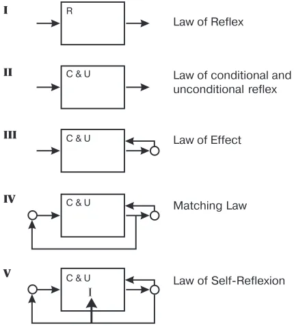
In the evolution of the science of behavior, one may see a clear logic which does not depend much on in individual preferences of researchers, neither on prohibitions on use introspective concepts (as for example, Pavlov’s avoiding such expression as “a dog noticed,” “a dog understood,” etc.). We single out four stages in the devel-opment of behaviorism and can see a move toward the fifth one, today (Fig. 1). Each stage can be described by a “law,” which expresses a rule of behavior of an organism in concise form.
At the first stage, which appeared in the Cartesian time, an organism was rep-resented as a black box with an input and output (here we use a metaphor belong-ing to later times). An organism’s life actions, called responses, correspond to the output, and the environment’s demands - to the input. A mechanism inside the box automatically transforms each demand into a response. This transformation was called reflex.
Pavlov’s (1927) discovery that reflexes are of two types: inborn and acquired, indicates the appearance of the second stage. The inborn reflexes were called un-conditional, and those acquired as the life experience were called conditional. The probabilistic models, as a rule, belong to the first or second stage. Unlike deter-ministic models, they describe statistical characteristics of stimulus-response rath-er than functional relation between a set of stimuli and a set of responses.
During the third stage, it was found that the automatic response to a stimulus may change becoming more effective. At the beginning of this stage was Thorndike (1932) who formulated The Law of Effect, which shows the ability of a living crea-ture to modify its response to a stimulus depending on its “effect.” For example, a cat’s organism in Thorndike puzzle box performs selections of successful manipu-lations with the lock and at the end of successive trials exits cage faster than at the beginning (see also Herrnstein, 1970; Williams, 1988).
generates a line of behavior which establishes a fixed ratio between a sequence of stimuli and a sequence of responses. A mathematical formula for this ratio has been called the Matching Law. Numerous attempt to explain this law in the frame-work of behaviorism have not given us a convincing explanation.
From the RIMS point of view, the Matching Law displays bipolarity and the law of self-reflexion (Lefebvre, 1999a; 2002). The concepts of the image of the self and intention lie beyond the vocabulary of behaviorism. Without broadening its vo-cabulary the science of behavior may not be able to explain the Matching Law. The broadening of behaviorism framework leads us toward the fifth stage which indi-cates merging of mentalism and behaviorism (Fig. 1).
Fig. 1. Logical stages in the development of behaviorism. The scheme does not reflect the time order of the ideas’ appearance. For example, Pavlov, Thorndike, Watson and Bechter-ev worked on their studies at about the same time, but contributions by early Watson and Bechterev belong to the first stage, by Pavlov to the second one, and by Thorndike to the third stage.
Law of Reflex
Law of conditional and unconditional reflex
Law of Effect
Matching Law
Law of Self-Reflexion R
C & U
C & U
C & U
C & U
I
I
II
III
IV
V
2. The Matching Law
rein-forcement is delivered. The mean interval between the appearance of grains can vary (Variable-Interval Schedules, VI). The experiment consisted of a series of ses-sions with fixed mean intervals for each key in each session. The pair of intervals were chosen in such a way that sometimes the reinforcement appeared more often in one key, and sometimes in the other.
It turned out that the birds choose the line of behavior such that the ratio of the numbers of pecks to the keys (B1 and B2) is approximately equal to the ratio of the numbers of corresponding reinforcements (r1 and r2):
Equation (2.1) was called the Matching Law. There were also experiments with rats and humans. Besides VI other schedules were also used. For example, in Vari-able-Ratio Schedule, VR, the mean number of pecks, necessary to receive rein-forcement, varied. The results of the experiments led to the formulation of the Generalized Matching Law (Baum, 1974):
where c and β are parameters which characterize a subject in a given experiment consisting of a sequence of sessions. Quite recently, Baum et al. (1999) suggested that (2.2) can be reduced to
where BP > BN. Variables with subscript P relate to the more often chosen alterna-tive, and those with N relate to less often chosen one. In his recent publication, Baum (2002) substituted condition BP > BN. with condition rP > rN.
Equations (2.1), (2.2) and (2.3) are particular cases of the more general equa-tion:
which represents the subjects’ behavior in the experiments described above (Davi-son & Jones, 1995; Baum & Aparicio, 1999).
3. The Attempts to explain the Matching Law within the Framework of the Science of Behavior
Why does equation (2.4) hold? It is natural to assume that it is a by-product of more fundamental processes (Williams, 1988). Baum and Aparicio (1999) gave the following interpretation which expresses the dominant point of view: ”Despite = . (2.1) Β1
Β2
r1 r2
= c ( )β , (2.2) Β1
Β2
r1 r2
= c ( ) , (2.3) ΒN
ΒP
rN rP
= c ( ), (2.4) Β1
Β2
claims to the contrary, all leading theories about operant choice may be seen as models of optimality” (p. 75). The idea of optimality is consonant with the main thesis of behaviorism, in accordance to which an animal is adapting to the environ-ment in a way that it looks rational and goal oriented.
There are numerous general and experimental arguments pro and contra the principle of optimality as an explanation of the Matching Law (Williams, 1988; Baum et al., 1999). The results of the experiments conducted by Mazur (1981) present a serious argument against the principle of optimality. The conditions of the experiments permitted the researchers to easily discover the pigeons tenden-cy to maximize the amount of food they received. Nevertheless, the birds did not choose the optimal strategy, they chose the strategies to make equation (2.4) hold instead.
Let us consider one more argument against the principle of optimality. Equa-tion (2.2), which describes the Generalized Matching Law, has two free parameters c and β. Their value must be found experimentally for each subject. There were many discussions concerning β (Baum, 1979; Wearden & Burgers, 1982; Aparicio, 2001), but c was considered just a scale coefficient connecting utility-values of re-inforcements from two different sources. A usual explanation of the necessity of its introduction can be clarified with the following example. Let a piece of food from the left food-hopper is 0.75 of that from the right one. If we write (2.1) for the “sum” of utilities, instead of the number of pieces (r1 and r2), we will obtain the following ratio:
= . (3.1) Β1
Β2
r1
0.75r2
Similar argumentation was used for the experiments in which the pieces of food were equal. In these cases, it was said that parameter c reflects a hidden factor which changes utility-measures of the same product from two different sources. Sometimes for the sake of saving this argumentation, the researchers had to as-sume that the organism of the subject was capable of finding statistical characteristics of non-simultaneous factors and reflecting them onto c. How else could they explain the fixed value of c in the experiments, in which one alternative was connected with schedule VI, and the other with schedule VR? (see, for example, Baum, 1974, Fig. 5.) The explanation of c constant value turns into an independent problem similar in its complexity with the explanation of the Matching Law. But if we reject the interpreta-tion of c as a scale coefficient, all the attempts to reduce the Matching Law to opti-mality look unconvincing.
4. RIMS
One of them plays the role of the positive pole and the other that of the negative pole. The subject is represented with the following equation:
X1 – x1 – (1– x1)(1– x2)M(x3) = 0 , (4.1)
where all variables and function M(x3) take on the values from interval [0,1] (Lefe-bvre, 1999b; 2001).
Variable X1 represents the subject’s executive system. Its value is the relative probability with which the subject’s executive system is ready to influence the pos-itive agency. Variable x3 corresponds to the subject’s model of the self. It represents the intentional domain of the subject. Its value is the relative probability with which the subject intends to influence the positive agency. The appearance of intention and the appearance of readiness are considered to be two independent events. For the sake of language simplicity, we will call X1 – readiness, and x3 – intention.
Variable x1 represents the relation between the subject and the positive agency in a given moment. Its value is interpreted in two ways. First, it is a relative proba-bility of the positive agency influencing the subject. Second, it is the subject’s re-quirement of the positive agency to influence him with this probability.
Variable x2 represents the subject’s experience. Its value is the integral estimation of the relative probability with which the positive agency influenced him in the past. Function M(x3) represents the subject’s prognostic activity. Its value is the sub-jective evaluation of the future positivity under condition that intention x3 turns into reality.
The environment may determine all values of the variables X1, x1, x2, x3 or only some of them. If the set of values determined by the environment is such that limita-tion (4.1) does not hold, we consider the subject disadapted. In the opposite case, we consider the subject adapted to the environment. The variables not determined by the environment may take on any values which do not violate (4.1).
If the value of x1 is determined by the environment, we interpret it as the influ-ence received from the environment. In the opposite case, it is interpreted as the subject’s need in the environment’s influence.
The subject adapted to the environment is called intentional if (4.1) is supple-mented with the following limitation:
X1 = x3 , (4.2)
that is, the intentional subject’s readiness is equal to its intention. The intentional subject’s choice will be called an intentional probabilistic choice.
Under condition (4.2) expression (4.1) turns into the following equation in relation to X1:
X1 = f(x1,x2) , (4.4) satisfying (4.3), we can exclude x3 from our considerations. RIMS then turns into a behavioristic model, all variables of which can be related to observable values.
If X1 is not an effective function of x1 and x2, we assume that the subject has the ability to make a choice, even probability of which cannot be predicted by external observers. We call this choice a free choice.
While modeling some psychological processes we may introduce more func-tional limitations on connections between variables X1, x1, x2, x3 to reflect subjects’ specific peculiarities. It follows from (4.1) that the following inequalities hold in-dependently from the type of function M(x3):
x1≤X1≤ 1 – x2 + x1x2 . (4.5) In the framework of this work, we consider function M(x3) to be linear and look as follows:
M(x3) = (1 – d)x3 , (4.6) where d ∈ [0,1]. The value of d is interpreted as an index of depression. This index lowers a degree of the positivity of the future. For example, when this index is maxi-mal, d = 1, function M(x3) ≡ 0, that is, the future looks negative for the subject. When d = 0, M(x3) ≡x3, that is, the degree of positivity of the future is equal to the value of intention. If (4.6) holds, (4.3) turns into equation in relation to X1:
X1 = x1 + (1 – x1)(1 – x2)(1 – d) X1, (4.6a) hence, with x1 + x2 + d > 0
When x1 = x2 = d = 0, the value of X1 is not a function of x1 and x2; so, in accordance with the definition, the subject is capable of making a free choice.
If x1 > 0, (4.7) can be represented as
Let us connect this equation with the number of the subject’s influence on the agencies and the number of the agencies influences on the subject as follows:
where N1 and N2 are the numbers of the subject’s influences on the positive and negative agencies, and n1 and n2 are the numbers of the positive and negative agen-cies’ influences on the subject. By substituting these values into (4.8), we obtain
X1= , x1 = , (4.8a) Ν1 + Ν2
Ν1
n1 + n2 n1
= (1 – (1 – x2)(1 – d))( ) . (4.8) X1
1 – X1
x1 1 – x1
= Ν p ( ) , (4.9) 1
Ν2
n1 n2
x1
where
p = 1 – (1 – x2)(1 – d). (4.10)
Equation (4.9) represents the intentional subject when M(x3) = (1 – d)x3 . On the other hand, (4.9) corresponds to the Generalized Matching Law (2.2) for β = 1. If in equation (2.2), B1 corresponds to the positive pole and B2 to the negative pole, then the value of p corresponds to free parameter c.
The values
will be called reinforcement densities D1 and D2. Now we write (4.9) as follows:
It follows from the equivalency of (4.11), (4.9), (4.8) and (4.7) that the subject is intentional if and only if (4.11) holds.
= p . (4.11)
D2 D1
5. Modeling the Experiment with Two Keys
We assume that in the experiments with the two keys, the subject’s activity aims not only at obtaining food, but also at generating a mixed state (see Introduction). First, an organism stabilizes the relative frequencies of contacts with the agencies by holding X1 = x3. After stabilization, frequency N1/(N1+N2) “turns” into the probability equal to the frequency, which characterizes the subject’s mixed state. Further we demonstrate that the experiment with two keys can be modeled with the help of RIMS.
The subject is placed into a cage with two keys each connected with a food-hopper. The subject’s pecks onto keys are reinforced by pieces of food but rarely. Each key has its own schedule of reinforcement (type VI or VR). The experiment consists of a series of sessions. In every session, the mean interval between rein-forcements is fixed for each key. Let suppose that
(1) The preparation of the subject to the experiment and the conditions of the experiment determine the value of the depression index d, being constant during the entire experiment.
(2) The following events take place at the beginning of each session:
(a) One key acquires the status of the positive agency, and the other one that of the negative agency.
(b) Variable x2 takes on a fixed value equal to or depending on the relative mean frequency of reinforcements in the previous sessions from the key, which in a given session plays the role the positive agency. If a given session is first, x2=1/2.
The goal of this process is to form and preserve the state in which an organism has the ability to make an intentional probabilistic choice. RIMS does not indi-= D1 and = D2 (4.10a) Ν1
n1
cate the strategy which the subject’s organism will choose to reach and hold equa-tion (4.9). It is possible that the subject controls equaequa-tion (4.11) for local densities in the way similar to the one described by the model of melioration (Rachlin, 1973; Vaughan, 1985).
6. The Patterns of Behavior Predicted by RIMS
We will call the alternative (key) richer if, in a given session, the subject behaves in such a way that this alternative is reinforced more often. In the framework of RIMS, the keys are polarized. One of them plays the role of the positive pole, and the other that of the negative pole. Consider three possible relations between polarization and richness along the set of sessions.
(A) One alternative is the positive pole in all sessions independently from be-ing richer or not.
(B) In each session, the least rich alternative is the positive pole. (C) In each session, the richer alternative is the positive pole.
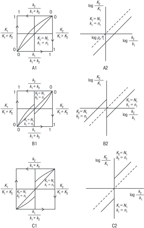
We will call one key right and the other left. Let K1 and K2 be the numbers of pecks to the right and left keys, and k1 and k2 the numbers of corresponding rein-forcements. Using functions (4.7) and (4.9) we will construct now a graph of K1/ (K1 + K2) depending on k1/(k1 + k2) and a graph of log(K2/K1) depending on log(k2/k1) for cases (A), (B) and (C). N1 and n1 relate to the positive pole, and N2 and n2 to the negative pole. Each graph corresponds to a set of sessions (Fig. 2). Graphs A1 and A2 map the case, when the right key plays the role of the posi-tive pole and the left one the role of the negaposi-tive pole, during the entire set of ses-sions
Graphs B1 and B2 map the case, in which the right or the left key corresponds to the positive pole only in those sessions in which it is not richer. Because of that, the graphs have a breach. Let us look at B1. For those sessions in which k1 < k2, the right key is the positive pole. At k1 = k2, there is a breach, corresponding to the reorientation of the poles. At k1 > k2, the left key is the positive pole. The logarith-mic graph B2 consists of two rays going at the angle of 450 to the horizontal axis.
The left ray corresponds to the sessions with the left key being the positive pole, and the right ray to those with the right one.
Graphs C1 and C2 map the case when one of the keys (right or left) is the positive pole only in those sessions in which it is richer than the other. Consider C1. When k1 > k2, the right key is the positive pole. At k1 = k2, as in B1, there is a breach. At k1 < k2 the left key is the positive pole. The logarithmic graph C2, as B2, consists of two rays.
Fig. 2. The patterns of behavior predicted by RIMS
A ray shift up or down on logarithmic graphs A2, B2 and C2 is predetermined by
p = 1 – (1 – x2)(1 – d). (6.1)
It is easy to see that p=1 only under condition that at least one of the values, x2 or d, is equal to 1. The value x2=1 means that the subject received all the preceding reinforcements from the key which is positive in the given session. In real experi-ments, the subjects always have some experience in receiving reinforcements from the negative key, as well. Thus, we have to consider x2 < 1.
K1= N1 k1 = n1
K1= N1 k1 = n1 K1 K2 log
log p { 0 0 1 1 0 0 1 1 0 0 1 1 0 0 1 1 K1= N1 k1 = n1
K2= N1 k2 = n1
k1 k2 log k1+ k2
k2
K1+ K2 K2
K2= N1 k2 = n1
K1= N1 k1 = n1
k1 k2 log B1 B2 A1 A2 K1 K2 log k1 k2 log K1 K2 log
K1= N1 k1 = n1 K2= N1 k2 = n1 k1+ k2
k2
k1+ k2 k1 K1+ K2
K1
K1+ K2 K2
k1+ k2 k2
k1+ k2 k1 K1+ K2
K1
K1+ K2 K2 K1= N1 k1 = n1
K2= N1 k2 = n1
C1 C2
k1+ k2 k1 K1+ K2
= . (7.2)
N1 + N2 N1
n1 + pn2 n1
Therefore, the ideal correspondence
may appear only at d = 1, that is, if the subject has been led to the state with the maximal index of depression. When d = 0, that is, the index of depression is mini-mal, the following equation is realized:
= (6.2) Ν1
Ν2
n1 n2
B1 B2 log
r1 r2 log B1+ B2
B1
r1+ r2 r1 1
0 1
(a) (b)
= x2 . (6.3) Ν1
Ν2
n1 n2
= . (7.1)
B1 + B2 B1
r1 + cr2 r1
Fig. 3. A type of experimental graphs corresponding to pattern A
In the framework of RIMS we interpret this pattern as follows: the key corre-sponding to B1 is the positive pole and c = p. Therefore (7.1) can be written as
7. The Patterns Observed
Pattern A is well known. It is usually described as a case of β= 1 in (2.2). This pattern appears under condition that left and right alternatives differ essentially. For example, the left key is under schedule VI, and the right one under VR (see Baum, 1974; Williams, 1988). In this case, a set of sessions can be described by (7.1), where c ≤ 1:
An analysis of the experiments, in which one key (say the left one) is controlled by schedule VI, and the other (right) by VR, demonstrates that VR key is the posi-tive pole, and VI one is the negative pole.
Pattern B is also known well. It is observed when alternatives do not differ but by the ratios of schedules. This observation made Baum et al. (1999, see also Baum, 2002).
This pattern, as Baum et al. noted, corresponds to cases with β < 1, if we de-scribe it with the Generalized Matching Law. The appearance of a twist inherent to this law may be explained as an approximation of broken graph 4(a) by a continu-ous power function (Fig. 5).
By analyzing graphs in Fig. 4 with RIMS we see that the positive pole corre-sponds to the alternative which is less reinforced. This peculiar fact, as we will show later, is a key fact for understanding the difference between utilitarian and deonto-logical aspects in animal behavior.
Pattern C can be seen rarely and only recently has been singled out as a special (Baum, 2002, Fig. 1). We can see an example of it in the experiment by Baum and Aparicio (1999) where one alternative was worked on VR-schedule with constant
Fig. 4. A type of experimental graphs corresponding to pattern B B1+ B2
B1
r1+ r2 r1 1
0 1
B1 B2 log
r1 r2 log
(a) (b)
0
Fig. 5. An approximation of a broken graph (Fig. 4a) by a continuous power function
0 1
1
B1+ B2 B1
mean ratio, and the other one – on VI-schedule and interval changing session by session. The data of this experiments (rats 102, 111, 120, 213) can be represented in the graph in Fig. 6:
Following Baum (2002), we may suppose that this pattern reveals itself in the experiments whose description with the Generalized Matching Law requires introduction of β > 1. As in pattern B, the appearance of a curve breach can be explained by approximation of graph 6(a) with a power function (Fig. 7).
The experiment by Baum and Aparicio (1999) and their analysis demonstrates that pattern C can be reduced to pattern A, if instead of location (right/left) alter-natives are coordinated by schedules (VR/VI). Then graph 6(a) looks like Fig. 8.
1
0 1
0
1
0 1
0 B1+ B2
B1
BVR+ BVI BVR
r1+ r2 r1
rVR+ rVI rVR
Fig.7. Approximation of broken graph Fig. 6(a) – with a continuous power
function
Fig.8. Pattern (A), corresponding to pattern C in Fig. 6(a) B1+ B2
B1
r1+ r2 r1 1
0 1
B1 B2 log
r1 r2 log
(a) (b)
0
Fig.6. A type of experimental graphs corresponding to pattern C
Pattern C may appear in the experiments when a factor which determines a positive-negative polarization of the alternatives in some sessions is connected with the left alternative and in the others with the right one.
vertical axis in Fig. 3(b). According to Williams (1988), when one key works un-der VI-schedule, and the other under VR-schedule, c = 0.59. Most pattern B data were treated under assumption that the Generalized Matching Law holds, be-cause of this it is close to impossible to extract the value of c from them. To find the value of c for pattern B using logarithmic data, we need to perform a linear approximation separately for the dots lying above the horizontal axis and those lying below it. Such a procedure was performed by Baum et al. (1999). We used their data and found the mean value of c = 0.58. In RIMS c corresponds to p found from (4.10).
Let us find now the mean value of the depression index d for this experiment assuming x2 = 0.5. Then (4.10) looks as follows:
0.59 = 1 – (1 – 1/2)(1 – d) , (7.3)
from where d= 0.18. Therefore, RIMS predicts that in this experiment, a pigeon’s prognostic model of the future can be represented as function m(x) = 0.82x.
8. Animals Deontological Evaluations
We would like to put forth a hypothesis that animals have ability to make bipolar, positive vs. negative evaluations analogous to (and perhaps preceding evolution of) the human moral evaluation good vs. bad. To find out how moral-like evaluations in animals are connected with the utilitarian preferences, let us consider ourselves first. Here is a specific case. In 1918, during the Civil War in Russia, the head of one family ends up in China, while his wife is left in Russia with six children; she is executed. The father finds a wealthy American, who with the risk to his life goes to Russia, finds children and brings all six of them to their father to China. Ten years later, with great difficulties, the same American helps them to move to the USA. The oldest of the saved children feels disappointed there.
Why America was not good for twenty-two-year old Mulia? Nostalgia? No. The thing was that the most important value for her - that of self-sacrifice - contradicted to the American style of life. Mulia was confused. An idea of “living for others”, natural to her, somehow could not be applied to America. Of course, Mr. Crane “sacrificed” a lot of time and money to charity (he was helping 50 more families to stand on their feet!). But his activity did not carry that special beauty of total self-sacrifice, admiration of which Mulia got with her mother’s milk? (Pann, 2003).
Let us make the next step and suppose that this mechanism has a deep biolog-ical nature, while it only looks culturally conditioned. In developing this idea we can hypothesize that birds and mammals have two systems of evaluations. The first system, utilitarian, reflects evaluations of the agencies related to the animal close biological needs. The second one, deontological, is connected with bipolar evalu-ations positive-negative on a larger time scale.
Consider, for example, a hungry animal choosing between two feeders. The first one contains more food, but the second one is more safe (say, hidden from view). In this case, the agency richer with food gets evaluation “negative” while the poorer one receives “positive” evaluation. Thus, animals’ “idealism” while being related to specific life-important evaluations, is nevertheless separated from this-minute preferences. We cannot exclude the possibility that this distinction is sup-ported by a special mental mechanism, whose work in humans reveals itself in a dramatic contrast between material and ideal values.
From this point of view, let us look at the patterns of behavior described in the previous sections. Pattern B appears when left and right food-hoppers differ only in their frequency of food delivering. In this case, as we found, the alternative which is less reinforced plays the role of the positive pole. We may hypothesize that this phenomenon reflects the work of the same mechanism which counterposes “dirty” money and “pure” intentions in humans. The alternative polarization opposite to their utilitarian preferences as food sources is analogous to the human act of puri-fication, that is, of separation good from practical profit. Let us emphasize that this happens if the alternatives differ only in the frequency of food delivery. If some “non-utilitarian” factor exists, which predetermines polarization of the alterna-tives, then the polarization remains the same during the entire session indepen-dently from reinforcement of the positive alternative. This conclusion results from the interpretation of patterns A and C.
9. Sacred Shift
Altruism is understood as spending one’s own resources in order to help others. But this is not the only form of sacrificial behavior. Voluntary expenditure of one’s finances and energy related to creation and support of religious and moral symbols is another form of sacrificial behavior. Everyone may cite an example of people who agree to perform work connected with higher values (say, building a cathedral) for smaller pay than they would require for similar work not connected with these values. RIMS offers explanation for this phenomenon. If we interpret N1 and N2 in (4.9) as the subject’s expenditures of appeals to the positive and negative agencies, and n1 and n2 as his revenues, then the ratios
and (9.0) Ν1
n1
express the mean payments the subject requires from the agencies for one appeal. It follows from (4.11) that
Therefore, it turns out that at average, the subject never requires more goods for one appeal from the positive agency than from the negative one. This conclusion is true not only for humans but for the rats and pigeons, as well.
Conclusion
We are convinced that we have a mental domain. This belief is based only on our own subjective experience. We do not have an operational criterion which would allow us to find out whether a particular organism or a technical device has an inner world. Or, on the other hand, are we observing an “inanimate” physical pro-cess. This problem extends beyond the framework of science and touches upon the core of our morality. We believe that a rat and a pigeon are able to suffer. But what about a fish or a bee, can they suffer? In this work, we put forth a hypothesis that the mental domain in living creatures appears at the same time as their ability to make a probabilistic choice. We have also substantiated an assumption that the creatures with mental a domain can “self-program.” That is, they can program themselves by downloading the values of probabilities with which they will make their choice. Furthermore, we have shown that the Matching Law is an external demonstration of this self-programming. If this hypothesis proves to be correct, then the Match-ing Law will turn into an operational criterion. We will thus have grounds to con-sider organisms, for which it holds, to have a mental domain.
Acknowledgements
I am thankful to William Baum and James Mazur for important clarifications and to Robert Kessel and William Palya for critical comments. I am grateful to my friends and colleagues, Jane Ryan, Stefan Schmidt, and Chris Weaver for valuable advice. I also want to thank Victorina Lefebvre, without whose help this work would not be done.
References
Adams-Webber, J. (1987). Comment on Lefebvre’s Model from the Perspective of Personal Construct Theory. Journal of Social and Biological Structures, 10, 177-189.
Adams-Webber, J. (1995). A Pragmatic Constructivist Gambit for Cognitive Scientists. PSYCOLOQUY, 6(34).
Adams-Webber, J. (1997). Self-reflexion in Evaluating Others. American Journal of Psychology,
110, 527-541.
Aparicio, C.F. (2001). Overmatching in Rats: The Barrier Choice Paradigm. Journal of the Experimental Analysis of Behavior, 75, 93-106.
Atkinson, R.C., Bower, G.H., and Crothers, E.J. (1965). An Introduction to Mathematical Learning Theory. New York: Wiley.
≤ . (9.1) N1
n1
Audley, R.J. (1960). A Stochastic Model for Individual Choice Behavior. Psychological Review,
67, 1-15.
Baker, H.D. (1999). The Good Samaritan: An Exemplary Narrative of Moral Choice. Proceedings of the Workshop on Multi-Reflexive Models of Agent Behavior. Los Alamos, NM: Army Research Laboratory, 63-68.
Batchelder, W.H. (1987). Some Critical Issues in Lefebvre’s Framework for Ethical Cognition and Reflexion. Journal of Social and Biological Structures, 10, 214-226.
Baum, W.M. (1974). On Two Types of Deviation from the Matching Law: Bias and Undermatching.
Journal of the Experimental Analysis of Behavior, 22, 231-242.
Baum, W.M. (1979). Matching, Undermatching, and Overmatching in Studies of Choice. Journal of the Experimental Analysis of Behavior, 32, 269-281.
Baum, W. M. (2002). From Molecular to Molar: A Paradigm Shift In Behavior Analysis. Journal of the Experimental Analysis of Behavior, 78, 95-116.
Baum, W.M. & Aparicio, C.F. (1999). Optimality and Concurrent Interval and Variable-Ratio Schedules. Journal of the Experimental Analysis of Behavior, 71, 75-89.
Baum, W. M., Schwendiman, J. W., and Bell, K. E. (1999). Choice, Contingency Discrimination, and Foraging Theory. Journal of the Experimental Analysis of Behavior, 71, 355-373. Bower, G.H. (1959). Choice-Point Behavior. In: Bush, R.R. & Estes, W.K. (Eds.), Studies in
Mathematical Learning Theory, Stanford: Stanford University Press.
Bradley, R.A. & Terry, M.E. (1952). Rank Analysis of Incomplete Block Design. The Method of Paired Comparisons I. Biometrika, 39, 324-345.
Davidson, D., Suppes, P., and Siegel, S. (1957). Decision Making. Stanford: Stanford Univ. Press. Davison, M. & Jones, B.M. (1995). A Quantitative Analysis of Extreme Choice. Journal of the
Experimental Analysis of Behavior, 64, 147-162.
Herrnstein, R.J. (1961). Relative and Absolute strength of Response As a Function of Frequency of Reinforcement. Journal of the Experimental Analysis of Behavior, 4, 267-272.
Herrnstein, R.J. (1970). On the Law of Effect. Journal of the Experimental Analysis of Behavior,
13, 243-266.
Kaiser, T.B. & Schmidt, S.E. (2003). Terrorist Recruitment and Reflexive Control. Journal of Reflexive Processes and Control, 3, 92-101.
Kauffman, L. (1990). Self and Mathematics. In Wheeler, H. (Ed.): The Structures of Human Reflexion, New York: Peter Lang.
Krylov, V.Yu. (1994). On One Model of Reflexive Behavior Distinct from Lefebvre Model. Applied Ergonomics, 1, 21-24.
LaBerge, D.L. (1962). A Recruitment Theory of Simple Behavior. Psychometrika, 27, 375-396. Lefebvre, V.A. (1965). On Self-reflexive and Self-organizing Systems, In: Problemy Issledovania Sistem i Struktur. Moscow: Izdatelstvo AN USSR. English translation in Applied Ergonomics, (1994), 1, 6-9.
Lefebvre, V.A. (1967). Konfliktuyushchie Struktury. Moscow: Vysshaya Shkola.
Lefebvre, V.A. (1972). A formal Method of Investigating Reflective Processes. General Systems,
XVII, 181-188.
Lefebvre, V.A. (1977a). The Structure of Awareness: Toward a Symbolic Language of Human Reflexion. Beverly Hills: Sage.
Lefebvre, V.A. (1977b). A Formal Approach to the Problem of Good and Evil. General Systems,
XXII, 183-185.
Lefebvre, V.A. (1980). An Algebraic Model of Ethical Cognition. Journal of Mathematical Psychology, 22, 83-120.
Lefebvre, V.A. (1987). The Fundamental Structures of Human Reflexion. Journal of Social and Biological Structures, 10, 129-175.
Lefebvre, V.A. (1992a). A Psychological Theory of Bipolarity and Reflexivity. Lewiston, N.Y.: The Edwin Mellen Press.
Lefebvre, V.A. (1999a). Categorization, Operant Matching, and Moral Choice. Institute for Mathematical and Behavioral Sciences, MBS, 99-14, UCI.
Lefebvre, V.A. (1999b). Sketch of Reflexive Game Theory. Proceedings of the Workshop on Multi-Reflexive Models of Agent Behavior. Los Alamos, NM: Army Research Laboratory, 1-40. Lefebvre, V.A. (2001). Algebra of Conscience, 2nd enlarged edition. Dordrecht:Kluwer Academic
Publishers. Expanded Russian translation (2003), Moscow: Cogito-Centre.
Lefebvre, V.A. (2002). The Law of Self-Reflexion. Journal of Reflexive Processes and Control, 1, 2, 91-100.
Lefebvre, V.A. & Adams-Webber, J. (2002). Function of Fast Reflexion in Bipolar choice. Reflexive Processes and Control, 1, 1, 29-40.
Levitin, L. (1987). Niels Bohr’s Atom and Vladimir Lefebvre’s “Inner Computer.” Journal of Social and Biological Structures, 10, 183-185.
Luce, R. D. (1959). Individual choice Behavior: A Theoretical Analysis. New York: Wiley. Mazur, J. E. (1981). Optimization Theory Fails to Predict Performance of Pigeons in a
Two-Response Situation. Science, 214, 823-825.
McClain, E. (1987). Comment on Vladimir Lefebvre’s Tonal Automata. Journal of Social and Biological Structures, 10, 2, 204-212.
Miller, L. D. & Sulcoski, M. F. (1999a). Reflexive Model of Human Behavior: Variations on Lefebvre’s Theme. Proceedings of the Workshop on Multi-Reflexive Models of Agent Behavior. Los Alamos, NM: Army Research Laboratory, 51-62.
Miller, L.D. & Sulcoski, M.F. (1999b). Application of Generalized Reflexive Behavior: Models for Situation-Specific Decisions. Proceedings of the Workshop on Multi-Reflexive Models of Agent Behavior. Los Alamos, NM: Army Research Laboratory, 69-94.
Mosteller, F. & Nogee, P. (1951). An Experimental Measurement of Utility. The Journal of Political Economy, 59, 371-404.
Pann, L. (2003). The Oldest Daughter. Novoye Russkoye Slovo, May 24-25. Pavlov, I.P. (1927). Conditioned Reflexes. Oxford: Oxford University Press.
Popper, K. (1992). Note in the Appendix to Lefebvre, V.A., A Psychological Theory of Bipolarity and Reflexivity. Lewiston, N.Y.: The Edwin Mellen Press.
Poulton, E.S. & Simmonds, D.C.V. (1985). Subjective Zeros, Subjectively Equal Stimulus Spacing, and Contraction Biases in Very First Judgments of Lightness. Perception & Psychophysics,
37, 420-428.
Rachlin, H. (1973). Contrast and Matching. Psychological Review, 80, 217-234.
Rapoport, A. (1990). Reflexion, Modeling, and Ethics. In Wheeler, H. (Ed.): The Structure of Human Reflexion. New York: Peter Lang.
Rapoport, A. (1996). Human Reflexion and the Anthropic Principle. PSYCOLOQUY, 6(37). Restle, F. (1961). Psychology of Judgment and Choice. New York: Wiley.
Ruddle, H., Bradshaw, C.M., Szabadi, E., and Bevan, P. (1979). Behaviour of Humans in Concurrent Schedules Programmed on Spatially Separated Operanda. Quarterly Journal of Experimental Psychology, 31, 509-517.
Savage, L.J. (1951). The Theory of Statistical Decision. American Statistical Association Journal,
46, 55-67.
Schreider, J.A. (1994). Fuzzy Sets and the Structure of Human Reflexion. Applied Ergonomics,
1, 19-20.
Schreider, J.A. (1998), Etika. Moscow: Tekst.
Skinner, B.F. (1938). The Behavior of Organisms: An Experimental Analysis. Appleton-Century-Crofts.
Spence, K.W. (1960). Conceptual Models of Spatial and Non-Spatial Selective Learning. In: Spence, K.W. (Ed.), Behavior Theory and Learning, Englewood Cliffs, N. J.: Prentice-Hall. Taran, T.A. (1999). The Formalization of Ethical Values in Models of Reflexive Behavior.
Proceedings of the Workshop on Multi-Reflexive Models of Agent Behavior. Los Alamos, NM: Army Research Laboratory, 95-108.
Thurstone, L.L. (1927). A Law of Comparative Judgment. Psychology Review. 34, 273-286. Tolman, E.C. (1932). Purposive Behavior in Animals and Men. New York: Appleton-Century-Crofts. Townsend, J.T. (1983). Vladimir A. Lefebvre. Algebra of Conscience (book review). Journal of
Mathematical Psychology, 27, 461-471.
Townsend, J.T. (1990). Lefebvre’s Human Reflexion and Its Scientific Acceptance in Psychology. In Wheeler, H. (Ed.): The Structures of Human Reflexion, New York: Peter Lang, 161-166. Vaughan, W. (1985). Choice: A Local Analysis. Journal of Experimental Analysis of Behavior, 43,
383-405.
von Neuman, J. & Morgenstern, O. (1947). Theory of Games and Economic Behavior. Princeton: Princeton University Press.
Wearden, J.H. & Burgess, I.S. (1982). Matching Since Baum (1979). Journal of the Experimental Analysis of Behavior, 28, 339-348.
Wheeler, H. (1987). A Constructional Biology of Hermeneutics. Journal of Social and Biological Structures, 10, 2, 103-123.
Williams, B.A. (1988). Reinforcement, Choice, and Response Strength. In: Atkinson, R.C., Herrnstein, R.J., Lindzey, G., Luce, R.D. (Eds.) Steven’s Handbook of Experimental Psychology, Vol.2, 167-244.