Modeling Potential C, N, H Content in Aboveground Biomass with Spectral Data from Sentinel 2a
Neftalí Reyes-Zurita1, Joaquín A. Rincón-Ramírez2, Gerardo Rodríguez-Ortiz1*, José R. Enríquez-del Valle1, Vicente A. Velasco-Velasco1, Ernesto Castañeda-Hidalgo1
1Tecnológico Nacional de México, Instituto Tecnológico del Valle de Oaxaca- Division de
Estudios de Posgrado e Investigación. Ex Hacienda de Nazareno s/n, Z.C. 71233 Xoxocotlán,
Oaxaca, México; 2Colegio de Postgraduados, Campus Tabasco, Periférico s/n, Z.C. 86500 H.
Cárdenas, México. *Corresponding author ([email protected]).
Abstract: Nutrient estimation in forest ecosystems through satellite images allows us to obtain accurate data, starting with data transformation from forest stands and the existing relationship with
the spectral information of the image through modeling. The objective of the study was to quantify
and validate the content of C, N, H in aboveground tree biomass in managed stands using spatial
modeling and satellite images. This study was conducted during 2017-2018 in managed forest
stands in San Juan Lachao, Oaxaca, Mexico. Fifteen 400 m2 experimental sites were selectively established, using a completely randomized experimental design of five silvicultural treatments
with three replications. As part of data preprocessing, normality and homogeneity of variances
assumptions were checked using the Shapiro-Wilk and Bartlett tests, respectively. From the pixels,
data of the average of Normalized Difference Vegetation Index (NDVI) that surrounded the
sampling sites were contrasted against the data obtained from forest inventory and the regression
models to estimate C, N, H and biomass were generated. Models were validated by NDVI. With
the models we estimated 0.95 t ha-1 biomass, which contains between 0.61 and 0.63 of C, 0.44-0.46 of N and 0.24 of H. The models generated had coefficients of determination (R2) of 0.85 to 0.87, which are significant parameters (p ≤ 0.0001). These results confirm that the use of Sentinel
satellite images in the estimation of these elements in forest ecosystems based on the relationship
between data inventory and the NDVI is highly reliable.
Keywords: Normalized difference vegetation index; San Juan Lachao; Satelital image.
1. Introduction
Sentinel 2A belongs to a program of new satellites developed by the European Union that
have been launched since 2015. As of 2016 the data can be used by any user at an international
level. These images have become an indispensable tool for the analysis of flora and fauna. Research
has been conducted with this sensor obtaining very satisfactory results due to its high resolution of
spatial, temporal, spectral and radiometric data [1]. Therefore, with multitemporal analysis, it is
possible to predict and prevent future risk scenarios [2].
In recent years, due to more in-depth understanding of the functional dynamics of both plant
physics and physiology, sensor technology has been used to evaluate plants indirectly and
non-destructively [3]. Satellite images have an extensive field of use, one of its main applications is
related to the possibility of observing changes in the vegetation under study over time [4].
Knowledge of the spectral models of different terrestrial covers permits adequate
interpretation of images coming from satellites. When characterizing vegetation, it can be observed
that when it is vigorous, it manifests very little energy in the region of the visible spectrum, mainly
due to absorption by chlorophyll to carry out photosynthesis, and therefore, a high proportion of
the electromagnetic radiation in the near-infrared region is reflected because of the characteristic
structure of leaf tissues. The use of satellite images is thus considered a tool for potential
quantification the nutrient content in vegetation. However, it is a great challenge to estimate macro
and micronutrients in heterogeneous mixed grassland [5].
The Normalized Difference Vegetation Index (NDVI) is a model used in agricultural and
the plant variable to be measured, such as plant biomass or vigor. The spectral response of healthy
vegetation shows a clear contrast in the visible spectrum, especially the red and the near infrared
(NIR) bands. In its interpretation, values below 0.1 are considered to correspond to water bodies
and bare soils, while higher values are indicators of the photosynthetic activity of different types
of vegetation [6]. This index was introduced with the objective of separating vegetation from the
brightness produced by the soil. It is based on the peculiar radiometric behavior of vegetation,
related to the photosynthetic activity and the plant´s leaf structure, which determine plant vigor [7].
In Mexico [8], Italy [9], Philippines [10], China [11], France [12] and other countries, work
has been done with the same satellite (NDVI) for analysis of urban vegetation, for soil
classification, for crop analysis, etc. Direct models center the data at a single point, while satellite
images (with correct processing of the image and dates as close as possible to the sampling dates)
have shown to improve the accuracy of forest biomass estimations [13].
Although it has been relegated due to the methodological difficulties involved when aiming
to produce detailed cartographic representation of vegetation variability or to provide relevant
information for forest management and decision-making at landscape scale [10], transformation of
the data recorded at the site (diameter at breast height and total height) and the relationship between
the data and the pixels provide the information needed for modeling the strata of a given forest in
terms of silviculture and ecology. In addition, with the satellite data, it is possible to estimate tree
height and update inventory or fill in nonexistent data effectively through correlation of pixel data
and points recorded in the stand inventory. Moreover, LIDAR measurements provide samples of
the forest structure that must be integrated with satellite images to predict and map the variations
of forest structure at the landscape scale [14].
Aboveground biomass is a fundamental element of forest ecosystems, very important for its
production capacity. Forest ecosystems store very significant amounts of gases with greenhouse
effect [15]. Estimation of forest stand biomass with accurate data from remote sensors is based on
a strong statistical relationship between C and the spectral response captured by the sensor as
spatially explicit knowledge [16].
Through research, it has been shown that forest reflectivity is assessed through the vertical
distribution of the tree strata [17]. Interactions between the structural variables of the inventory
data such as height, basal area, density, age and biomass at the time of modeling with satellite
images have also been detected [18].
Planning forestry activities requires information such as geographical features. In addition to
thematic maps that support decision-making, new alternatives have been adopted, as is the case in
northwestern Mexico where Landsat ETM satellite images from 2001 were used to optimize
forestry planning [19].
The community San Juan Lachao has large forest areas that are geographically difficult to
access. This community is a pioneer in the commercialization of C bonds (Carboin) in the
international voluntary market, through development of the project under the forest protocol for
Mexico of the Climate Action Reserve. The community are interested in constantly improving their
methods of evaluating their natural resources. In this context, the use of Sentinel satellite images
presents an alternative that saves time and resources in evaluating natural and environmental
resources. For this reason, the objective of this study was to quantify and validate the C, N and H
content in aboveground tree biomass in different silvicultural treatments using spatial modeling
3. Material and Methods
3.1. Study Area
The present research was carried out during 2017-2018 in the timber harvesting stands of San
Juan Lachao, Oaxaca, in southern Mexico. The stands are located at an average altitude of 1885 m
on slopes between 20-40%. Geographically, they are located between the coordinates: 16° 12'
42.66" N and 97° 05' 50.46" W. Predominant climate is warm subhumid with average annual
temperature of 22 ºC; precipitation is abundant between May and September and averages 2,500
mm per year.
2.2. Experimental Sites
Fifteen experimental units of 400 m2 were selectively established in 2017, using a completely randomized experimental design in five silvicultural treatments and three repetitions. The sites
were located spatially with a GPS (global positioning system) (Garmin Trex 30, USA). A forestry
tree inventory was carried out, obtaining the following variables: diameter at breast height (DBH,
cm) and total height (TH, m), both measured with a diametric tape (Jackson, MS 800-647-5368)
and clinometer (PM-5 360 PC).
2.3 Nutrients in Aboveground Biomass
In the arboreal compartment, the total tree volume of the pines and broadleaf species was
calculated with the Schumacher-Hall model (allometric) [20] (Eq 1).
……… Eq. 1
Where: v(st) = stem total volumen outside bark (m3), DBH = diameter at breast height (cm), TH =
total height (m), βi = regression coefficient.
To estimate the biomass of the different tree parts, a sample of approximately 100 g was
extracted from each part and kept in a tagged paper bag to determine fresh weight (FW, kg) and
dry weight (DW, kg) after drying for six days at temperature between 75 ºC and 100 ºC. The total
( )
1 2 2
biomass of each component was obtained by conversion factors (DW/FW), using the
Chávez-Pascual [21]methodology. Laboratory analyses were performed in order to obtain the nutrient
content in plant samples with an elemental organic analyzer PE 2400, series II (Eq 2).
100
i
nc n = B
……….. Eq. 2
Where: ni= nutrient (kg), nc = nutrient content (%), B = biomass (kg).
2.4 Spectral data Sentinel 2A
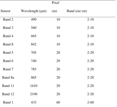
The multispectral image was obtained from the Sentinel Scientific Data Hub web site. The
sensor manages 13 bands in the visible spectrum (Table 1).
Table 1. Technical characteristics of Sentinel 2A.
Sensor Wavelength (μm)
Pixel
(m) Band size (m)
Band 2 490 10 2-10
Band 3 560 10 2-10
Band 4 665 10 2-10
Band 8 842 10 2-10
Band 5 705 20 2-20
Band 6 740 20 2-20
Band 7 783 20 2-20
Band 8a 865 20 2-20
Band 11 1610 20 2-20
Band 12 2190 20 2-20
Band 9 940 60 2-60
Band 10 1375 60 2-60
Thirteen bands were processed using QGIS 2.18.17® software. First, as part of
preprocessing, atmospheric and geometric corrections were made, and then the NDVI was
calculated (Eq 3). Two satellite bands were chosen: bands 4 and 8 with 10 m of spatial resolution.
Finally, in each georeferenced sampling site, the average of the surrounding pixels was obtained
using a 9×9 window, where the central pixel corresponded to the inventoried site; with this average,
the correlation between pixels and elements such as C, N, H and biomass was made.
NDVI NIR R NIR R
− =
+ ………Eq. 3
Where: NDVI = normalized difference vegetation index, NIR = near infrared, R = red.
The indexes were constructed in order to highlight some characteristics of the vegetation,
which is mainly a function of the chlorophyll, cell structure and water content of the vegetation
[22]. The indexes are more sensitive in some parts of the electromagnetic spectrum and better
detected in specific bands [23].
2.5 Data Analysis
A database was integrated with which regression models per tree were tested. The dependent
variable was the value of the pixels and the independent variables were C, H, N and biomass (Table
1). The analyses were carried out with SAS [24] statistical software. Assumptions of normality and
homogeneity of variances were verified with the Shapiro-Wilk (UNIVARIATE procedure) and
Bartlett tests, respectively. The models were adjusted using the MODEL procedure and selected
based on their statistical indicators. A simple linear model was used for C, N and biomass and
Results
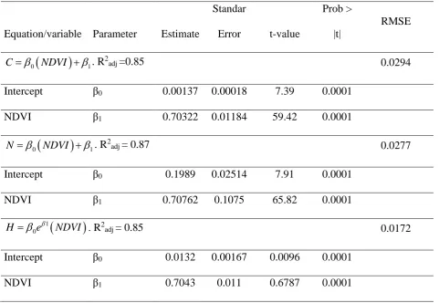
The models that best estimated C, N, H and biomass from spectral data were the simple linear
and the exponential regression models. The root of mean square error (RMSE) showed low values,
between 0.01 and 0.02, indicative of good fit. The NDVI spectral data explained 85% of the
variation in C, H and biomass and 87% of the variation in N; in all cases, variation was significant
(p = 0.0001). In this way, the parameters (β0 and β1) integrated to estimate the nutrient contents
and biomass were essential in the models (p = 0.0001).
The NDVI based on the reflectivity of the Sentinel 4 and 8 bands were those that satisfactorily
described the elements’ behavior due to the strong energy absorption caused by the vigorous
healthy vegetation, chlorophyll absorption and moisture present in the vegetation (Table 2).
Table 2. Regression models for nutrients and biomass.
Equation/variable Parameter Estimate
Standar
Error t-value
Prob >
|t|
RMSE
(
)
0 1
C= NDVI + . R2adj=0.85 0.0294
Intercept β0 0.00137 0.00018 7.39 0.0001
NDVI β1 0.70322 0.01184 59.42 0.0001
(
)
0 1
N = NDVI + . R2adj= 0.87 0.0277
Intercept β0 0.1989 0.02514 7.91 0.0001
NDVI β1 0.70762 0.1075 65.82 0.0001
(
)
1 0
H = e NDVI . R2adj= 0.85 0.0172
Intercept β0 0.0132 0.00167 0.0096 0.0001
(
)
0 1
B= NDVI + . R2adj=0.85 0.0293
Intercept β0 0.0006 0.00007 7.42 0.0001
NDVI β1 0.7029 0.01182 59.47 0.0001
C, N, H, B = carbón, nitrogen, hydrogen and biomass (kg), β0,1,2,3 = regression parameters, NDVI
= normalized difference vegetation index; RMSE = root mean square of error; R2adj= adjusted
coefficient of determination.
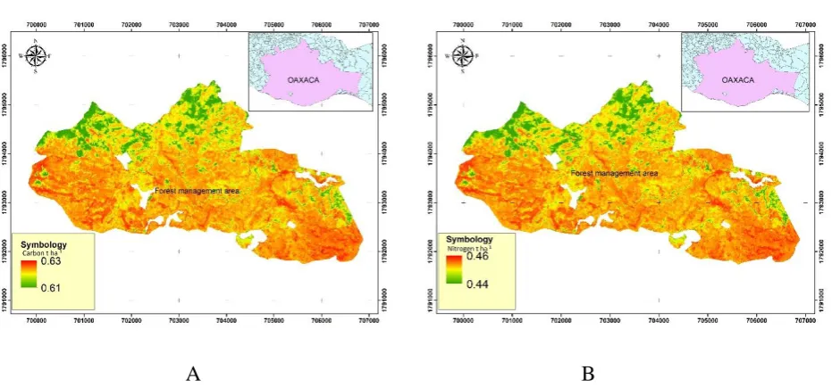
The modeled C storage potential of the stands with silvicultural treatment was 0.63 t ha-1 in the high areas where pine-oak is the predominant vegetation. In the stands intervened in the last
two years growing in wet climate, modeled potential C storage was 0.61 t C ha-1, due to the variation in silvicultural treatments and the type of dominant vegetation and climate. N is the
second most important element in the forest under study, which generates values between 0.44 t
ha-1 and 0.46 t ha-1. These values are high compared with the other evaluated nutrients. This variability may be because the silvicultural regimes were applied in different periods (2012 to
2015) (Figure 1).
A B
Hydrogen is one of the scarcest elements, found in small proportions in the forest. The model result
obtained in the managed stands was 0.22 t H ha-1 to 0.24 t H ha-1.
Biomass expansion was similar obtaining between 0.93 t ha-1 and 0.95 t ha-1. The areas with the least amount of biomass are stands that were intervened in 2015 and where oak-pine vegetation
predominates (Figure 2).
Figure 2. Hydrogen (A) and aboveground biomass (B) expansion at area under forest management.
4. Discussion
The need to know and simulate the different behaviors associated with the different
vegetation changes has been increasing. One of the first processes is observation; then comes
experimentation, and finally satellite images [25, 26] to obtain geolocated information, especially
in large areas of difficult access [27]. To make the most accurate C estimation, the spatial resolution
of the satellite image becomes a key factor in validating models. A study done by Yan [28] working
with resolutions between 30 and 1000 m2, used a model that showed high coefficients of variation as the image resolution decreased. The results of our investigation was 5.55 (CV) with a 20×20 m
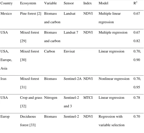
Results of studies carried out in Mexico, the United States, Europe, Iran and Asia, with
different satellites such as Sentinel 2 and 3, Landsat and Envisat, using statistical models, have
similar coefficients of determination, when compared with the results obtained in our research.
This highlights the fact that Sentinel sensors present differences relative to others, that is, it is much
better to make these types of estimates in forest ecosystems (Table 3).
Table 3. Use of different sensors in the C, N, H and biomass estimation.
Country Ecosystem Variable Sensor Index Model R2
Mexico Pine forest [2] Biomass
and carbon
Landsat NDVI Multiple linear
regression
0.67
USA Mixed forest
[29]
Biomass
and carbon
Landsat 7 NDVI Multiple regression 0.67
0.82 USA, Europe, Asia Mixed forest [30]
Carbon Envisat Linear regression 0.70,
0.90
Iran Mixed forest
[31]
Biomass Sentinel-2A NDVI Nonlinear regression 0.70,
0.95
USA Crop and grass
[32]
Nitrogen Sentinel-2
and 3
MTCI Linear regression 0.78
Europ Deciduous
forest [33]
Biomass Sentinel-2 NDVI Regression with
variable selection
0.70
The models generated from Sentinel 2a images for C estimation presented an R2 = 0.85, which is similar to research work carried out in southern Sweden with MODIS satellite images that
obtained 0.76 and 0.85 t ha-1 in the CO2 with NDVI estimation [34, 35].
Indirect estimation of C and forest variability is done with different methods and technologies
[36] from different variables, either height [37, 38] or biomass, which was the methodology used
in our investigation.
In estimating N with NDVI, it has been shown that reflectivity in some parts of the
electromagnetic spectrum is highly correlated with the N percentage measured in the stand at tree
level [39, 40]. In our research it produced an R2 = 0.87, comparable with the results of Pellissier [41] and Wang [42] in mixed temperate forest. Comparing the results generated in agricultural
areas with airborne hyperspectral images, we had an adjustment of R2 = 0.79, suggesting that the Sentinel 2a images estimate nutrient contents much better. Moreover, comparing the results
obtained by Ewald [43] with the Lidar data (R2 = 0.63), with the images obtained from Sentinel, more robust models can be generated to predict the aforementioned variables.
For this reason, the use of remote sensing in nutrient quantification and also in forest
management to estimate forest productivity in large areas to support establishing inventory control
points has boomed [44]. The result obtained in H quantification was 0.22 t ha-1, through pixel ratio,
to 0.24 t ha-1, obtained from the samples collected in the stand. Norverto [45] mentions that H is one of the scarcest elements; in a complete tree 6% can be found, depending on the species.
The different satellite images provide very accurate information at the local, regional and
national level if their methodology is followed correctly [28]. The biomass estimated through the
This difference could be due, first, to the fact that the MODIS sensor spatial resolution is
lower than that of Sentinel and, second, to its smaller R2 = 0.62 with multiple regression. It may also vary depending on vegetation type and the site condition. For example, Ruiz [47] obtained an
R2 = 0.89 in Pinus halepensis Mill, while Méndez [48], who used the ALOS-PALSAR sensor found R2 = 0.63 in pine species, and Cáceres [49] in an analysis of temporal behavior of grass
biomass in Honduras obtained an R2 = 0.82 from the biomass and the spectral index (SAVI) ratio with simple linear regression using Sentinel 2ª images. However, in the biomass quantification of
managed forest areas of this study, a coefficient of R2 = 0.85 was obtained (Table 1). Comparing the results with Vaglio [33] of R2 from 0.70 to 0.75 (Table 2) demonstrates that this satellite is a better biomass predictor.
5. Conclusions
Estimates carried out using statistical models with spectral data in an area of stands managed
under silvicultural regimes at San Juan Lachao in southern Mexico, showed similar levels of C
(0.63 t ha-1), while nitrogen was 0.46 t ha-1 on average. Hydrogen was lower than 0.24 t ha-1, being one of the scarcest elements. Both the regression models and their parameters (β0 and β1) showed
significant estimates (p = 0.0001) of the nutrients and biomass because the images used have a
resolution of 10, 20 and 60 m, which is a key point in selecting the sensor. Spatial modeling of
aboveground tree biomass and nutrients with Sentinel 2a images is reliable for use in stands under
silvicultural regimes.
Supplementary Materials: Excel® data base of contents of biomass, C, N and H.
Acknowledgments: We would like to acknowledge the Community of San Juan Lachao and Conacyt for funding the scholarship for the first author.
the field data collection, analyzed the data and wrote the manuscript. J.R. E-V. and V.A. V-V
assisted in analysis of the results and wrote the manuscript. And E. C-H. revised the manuscript.
Conflicts of Interest: The authors declare no conflict of interest.
References
1. Muñoz, R. C. A.; Treviño, G. E. J.; Verástegui, C J.; Jiménez, P. J.; Aguirre, C. O. A.
Desarrollo de un modelo espacial para la evaluación del peligro de incendios forestales en la
Sierra Madre Oriental de México. Investigaciones Geográficas 2005, 56, 101–117.
2. Martínez, B. R. A.; Aguirre, C. O. A.; Vargas, L. B.; Jiménez, J,; Treviño, G. E. J.; Yerena, Y.
J. I. Modelación de biomasa y carbono arbóreo aéreo en bosques del estado de Durango.
Revista Mexicana de Ciencias Forestales 2016, 7(35), 91–106.
3. Porras, A. G. Potencialidad y nuevas orientaciones en el uso de la teledetección en agricultura
y selvicultura. Ambienta 2013, 105, 6–15.
4. Baccini, A.; Friedl, M. A.; Woodcock, C. E.; Warbington, R. Forest biomass estimation over
regional scales using multisource data. Geophysical Research Letters 2004, 31(10), 2–5.
https://doi.org/10.1029/2004GL019782
5. Paruelo, J. M. La caracterización funcional de ecosistemas mediante sensores remotos.
Ecosistemas 2008, 17(3), 4–22.
6. Meneses-Tovar, C. L. El índice normalizado diferencial de la vegetación como indicador de
la degradacion de los bosques. Unasylva 2011, 62(238), 39–46.
7. Peña-Barragán, J. M.; Ngugi, M. K.; Plant, R. E.; Six, J. Object-based crop identification using
multiple vegetation indices, textural features and crop phenology. Remote Sensing of
Environment 2011, 115(6), 1301–1316. https://doi.org/10.1016/j.rse.2011.01.009
8. Sowter, A.; Bin, C.A. M.; Cigna, F.; Marsh, S.; Athab, A.; Alshammari, L. Mexico City land
(ISBAS) technique. International Journal of Applied Earth Observation and Geoinformation
2016, 52, 230–242. https://doi.org/10.1016/j.jag.2016.06.015
9. Pulvirenti, L.; Squicciarino, G.; Cenci, L.; Boni, G.; Pierdicca, N.; Chini, M.; … Campanella,
P. A surface soil moisture mapping service at national (Italian) scale based on Sentinel-1 data.
Environmental Modelling and Software 2018, 102, 13–28.
https://doi.org/10.1016/j.envsoft.2017.12.022
10.Castillo, J. A. A.; Apan, A. A.; Maraseni, T. N.; Salmo, S. G. Estimation and mapping of
above-ground biomass of mangrove forests and their replacement land uses in the Philippines
using Sentinel imagery. ISPRS Journal of Photogrammetry and Remote Sensing 2017, 134,
70–85. https://doi.org/10.1016/j.isprsjprs.2017.10.016
11.Li, F.; Song, G.; Liujun, Z.; Yanan, Z.; Di, L. Urban vegetation phenology analysis using high
spatio-temporal NDVI time series. Urban Forestry and Urban Greening 2017, 25, 43–57.
https://doi.org/10.1016/j.ufug.2017.05.001
12.Veloso, A.; Mermoz, S.; Bouvet, A.; Le-Toan, T.; Planells, M.; Dejoux, J.F.; Ceschia, E.
Understanding the temporal behavior of crops using Sentinel-1 and Sentinel-2-like data for
agricultural applications. Remote Sensing of Environment 2017, 199, 415–426.
https://doi.org/10.1016/J.RSE.2017.07.015
13.Gómez, C.; White, J. C.; Wulder, M. A.; Alejandro, P. Historical forest biomass dynamics
modelled with Landsat spectral trajectories. ISPRS Journal of Photogrammetry and Remote
Sensing 2014, 93, 14–28. https://doi.org/10.1016/j.isprsjprs.2014.03.008
14.Cigna, F.; Sowter, A. The relationship between intermittent coherence and precision of ISBAS
InSAR ground motion velocities: ERS-1/2 case studies in the UK. Remote Sensing of
Environment 2017, 202, 177–198. https://doi.org/10.1016/j.rse.2017.05.016
marco del cambio climático Forest Monitoring with Remote Sensing Within the Framework
of Climate Change. Revista UniveRsidad en Diálogo 2016, 6(2), 59–73.
https://doi.org/10.15359/udre.6-2.4
16.Lees, K. J.; Quaife, T.; Artz, R. R. E.; Khomik, M.; Clark, J. M. Potential for using remote
sensing to estimate carbon fluxes across northern peatlands – A review. Science of the Total
Environment 2018, 615, 857–874. https://doi.org/10.1016/j.scitotenv.2017.09.103
17.Wang, Q.; Li, P. Canopy vertical heterogeneity plays a critical role in reflectance simulation.
Agricultural and Forest Meteorology 2013, 169, 111–121.
https://doi.org/10.1016/j.agrformet.2012.10.004
18.Palestina, R. A.; Equihua, M.; Pérez-Maqueo, O. M. Influencia de la complejidad estructural
del dosel en la reflectancia de datos Landsat TM. Madera y Bosques 2015, 21(1), 63–75.
19.Ancira-Sánchez, L.; Treviño-Garza, J. E. Using satellite images for forest management in
northeast Mexico. Madera y Bosques 2015, 21(1), 77–91.
20.Corral, R. J. J.; Vargas, L. B. Sistema biométrico para la planeación del manejo forestal
sustentable de los ecosistemas con potencial maderable en México (2013-C01-209772).
Oaxaca, México, 2013.
21.Chávez-Pascual, E. Y.; Rodríguez-Ortiz, G.; Enríquez-del Valle, J. R.; Velasco-Velasco, V.
A.; Gómez-Cárdenas, M. Compartimentos de biomasa aérea en rodales de Pinus oaxacana
bajo tratamientos silvícolas. Madera y Bosques 2017, 23(3), 147-161.
doi:10.21829/myb.2017.2331627
22.Soria, R. J.; Granados, R. R. Relación entre los índices de vegetación obtenidos de los sensores
AVHRR del satélite NOAA y TM del Landsat. Ciencia Ergo Sum 2005, 12(2), 167–174.
23.Cohen, W. B.; Goward, S. N. Landsat’s role in ecological applications of remote sensing.
24.SAS Institute Inc. SAS/ETS 9.3 User´s Guide. SAS Institute, Cary, NC. USA, 2011.
25.Alton, P. B. Decadal trends in photosynthetic capacity and leaf area index inferred from
satellite remote sensing for global vegetation types. Agricultural and Forest Meteorology
2018, 250-251, 361-375. https://doi.org/10.1016/j.agrformet.2017.11.020
26.Huesca, M.; García, M.; Roth, K. L.; Casas, A.; Ustin, S. L. Canopy structural attributes
derived from AVIRIS imaging spectroscopy data in a mixed broadleaf/conifer forest. Remote
Sensing of Environment 2016, 182, 208–226. https://doi.org/10.1016/j.rse.2016.04.020
27.Sastre, L. F. S.; Marcos-Robles, J. L.; Llorente, E. H.; Navarro, S. H.; Prieto, P. C. Aplicación
de tecnologías de teledetección al estudio de biomasa forestal. Revista Iberica de Sistemas y
Tecnologias de Información 2016, 19, 61–76. https://doi.org/10.17013/risti.19.61-76
28.Yan, E.; Lin, H.; Wang, G.; Sun, H. Multi-resolution mapping and accuracy assessment of
forest carbon density by combining image and plot data from a nested and clustering sampling
design. Remote Sensing 2016, 8(7), 571. https://doi.org/10.3390/rs8070571
29.Zheng, D.; Rademacher, J.; Chen, J.; Crow, T.; Bresee, M.; Le Moine, J.; Ryu, S. R. Estimating
aboveground biomass using Landsat 7 ETM+ data across a managed landscape in northern
Wisconsin, USA. Remote Sensing of Environment 2004, 93(3), 402–411.
https://doi.org/10.1016/j.rse.2004.08.008
30.Thurner, M.; Beer, C.; Santoro, M.; Carvalhais, N.; Wutzler, T.; Schepaschenko, D.; …
Schmullius, C. Carbon stock and density of northern boreal and temperate forests. Global
Ecology and Biogeography 2014, 23(3), 297–310. https://doi.org/10.1111/geb.12125
31.Vafaei, S.; Soosani, J.; Adeli, K.; Fadaei, H.; Naghavi, H.; Pham, T. D.; Bui, D. T. Improving
accuracy estimation of Forest Aboveground Biomass based on incorporation of ALOS-2
PALSAR-2 and Sentinel-2A imagery and machine learning: A case study of the Hyrcanian
32.Clevers, J.G.P.W.; Gitelson, A.A. Remote estimation of crop and grass chlorophyll and
nitrogen content using red-edge bands on Sentinel-2 and -3. International Journal of Applied
Earth Observation and Geoinformation 2013, 23, 344–351.
http://dx.doi.org/10.1016/j.jag.2012.10.008
33.Vaglio, L. G.; Balling, J.; Corona, P.; Mattioli, W.; Papale, D.; Puletti, P.; Rizzo, M.;
Truckenbrodt, J. Y.; Urban, M. Above-ground biomass prediction by Sentinel-1 multitemporal
data in central Italy with integration of ALOS2 and Sentinel-2 data. J. Appl. Remote Sens.
2018, 12(1), 1-19 doi: 10.1117/1.JRS.12.016008.
34.Schubert, P.; Eklundh, L.; Lund, M.; Nilsson, M. Estimating northern peatland CO2 exchange
from MODIS time series data. Remote Sensing of Environment 2010, 114(6), 1178–1189.
https://doi.org/10.1016/j.rse.2010.01.005
35.Liu, N.; Harper, R. J.; Handcock, R. N.; Evans, B.; Sochacki, S. J.; Dell, B.; … Liu, S. Seasonal
timing for estimating carbon mitigation in revegetation of abandoned agricultural land with
high spatial resolution remote sensing. Remote Sensing 2017, 9(6), 545.
https://doi.org/10.3390/rs9060545}
36.Jiang, Q.; Chen, Y.; Guo, L.; Fei, T.; Qi, K. Estimating soil organic carbon of cropland soil at
different levels of soil moisture using VIS-NIR spectroscopy. Remote Sensing 2016, 8(9), 755.
https://doi.org/10.3390/rs8090755
37.Nunes, M. H.; Ewers, R. M.; Turner, E. C.; Coomes, D. A. Mapping aboveground carbon in
oil palm plantations using LiDAR: A comparison of tree-centric versus area-based approaches.
Remote Sensing 2017, 9(8), 1–13. https://doi.org/10.3390/rs9080816
38.Solberg, S.; May, J.; Bogren, W.; Breidenbach, J.; Torp, T.; Gizachew, B. Interferometric SAR
DEMs for forest change in Uganda 2000-2012. Remote Sensing 2018, 10(2, 228.
39.García, M. A.; Pérez, C. F.; de la Riva, F. J. Evaluación de los recursos de biomasa residual
forestal mediante imágenes del satélite Landsat y Sig. GeoFocus 2006, 6, 205–230.
40.Lepine, L. C.; Ollinger, S. V.; Ouimette, A. P.; Martin, M. E. Examining spectral reflectance
features related to foliar nitrogen in forests: Implications for broad-scale nitrogen mapping.
Remote Sensing of Environment 2016, 173, 174–186.
https://doi.org/10.1016/j.rse.2015.11.028
41.Pellissier, P. A.; Ollinger, S. V.; Lepine, L. C.; Palace, M. W.; McDowell, W. H. Remote
sensing of foliar nitrogen in cultivated grasslands of human dominated landscapes. Remote
Sensing of Environment 2015, 167, 88–97. https://doi.org/10.1016/j.rse.2015.06.009
42.Wang, Z.; Wang, T.; Darvishzadeh, R.; Skidmore, A. K.; Jones, S.; Suarez, L.; … Hearne, J.
Vegetation indices for mapping canopy foliar nitrogen in a mixed temperate forest. Remote
Sensing 2016, 8(6), 1–20. https://doi.org/10.3390/rs8060491
43.Ewald, M.; Aerts, R.; Lenoir, J.; Fassnacht, F. E.; Nicolas, M.; Skowronek, S.,; … Schmidtlein,
S. LiDAR derived forest structure data improves predictions of canopy N and P concentrations
from imaging spectroscopy. Remote Sensing of Environment 2018, 211, 13–25.
https://doi.org/10.1016/j.rse.2018.03.038
44.Smith, M. L.; Ollinger, S. V.; Martin, M. E.; Aber, J. D.; Hallett, R. A.; Goodale, C. L. Direct
Estimation of Aboveground Forest Productivity through Hyperspectral Remote Sensing of
Canopy Nitrogen. Ecological Applications 2013, 12(5), 1286–1302.
45.Norverto, A. C. La fijación de CO2 en plantaciones forestales y en productos de maderas en
Argentina. Proyecto Forestal de Desarrollo Secretaria de Agricultura, Ganadería, Pesca y
Alimentos 2013, 1-13.
46.Lumbierres, M.; Méndez, P.; Bustamante, J.; Soriguer, R.; Santamaría, L. Modeling Biomass
Sensing 2017, 9(4), 392. https://doi.org/10.3390/rs9040392
47.Ruiz, D. D.; Gracia, T. L.; Gracia, A. L. M.; Fernández, J. de la R. Estimación de la pérdida
de biomasa y de las emisiones de CO2 generadas por la combustión de masas forestales de
Pinus halepensis Mill. en el incendio de Luna (Aragón), mediante datos LiDAR-PNOA. XVII
Congreso Nacional de Tecnologías de Información Geográfica, España 2016, 83–88.
48.Méndez, E.; Valés, J. J.; Pino, I.; Granado, L.; Montoya, G.; Prieto, R.; … Suárez, J.
Determinación de biomasa forestal mediante la utilización de técnicas de teledetección con
imágenes radar. Estudio piloto en ámbito de la provincia de Huelva. Revista de Teledeteccion
2016, 45, 71–86. https://doi.org/10.4995/raet.2016.3984}
49.Cáceres, J. D. Análisis del comportamiento temporal de la biomasa en pastos del Departamento
de Olancho en el contexto del cambio global – Fase II. Revista de Ciencias Espaciales 2013,