S. Werner (ed.),Proceedings of the 15th NODALIDA conference, Joensuu 2005, Ling@JoY 1, 2006, pp. 88–93
analogical modeling and memory based learning
Christer Johansson & Lars G. Johnsen
Dept. of Linguistics and Literature
University of Bergen
N-5007 Bergen, Norway
{christer.johansson, lars.johnsen}@lili.uib.no
Abstract
Analogical modeling (AM) is a mem-ory based model. Known algorithms implementing AM depend on investi-gating all combinations of matching features, which in the worst case is exponential (O(2n)). We formulate a representation theorem on analogical modeling which is used for implement-ing a range of approximations to AM with a much lower complexity. We will demonstrate how our model can be modified to reach better performance than the original AM model a popular categorization task (chunk tagging).
1
Introduction
Analogical modeling (AM) is a method to evalu-ate the analogical support for a classification (Skousen, 1989; Skousen, 1992; Skousen et al., 2002), which is compatible with psycho-linguistic data (Chandler, 2002; Eddington, 2002; Mudrow, 2002, inter al.). Chandler (1993) propose it as an alternative to rule based and connectionist models of language process-ing and acquisition.
AM has also been used within Optimality Theory (Myers, 2002) and similar exemplar-based studies have looked at the development of phonological regularities with the number of exemplars (Pierrehumbert, 2001). AM defines a natural statistic, which can be implemented by comparisons of subsets of linguistic variables, without numerical calculations (Skousen, 1992; Skousen, 2002).
The original AM model compares all subsets of investigated variables. This causes an expo-nential explosion in the number of comparisons. This has made it difficult to investigate large models with many variables (> 10) and large
databases. Johnsen & Johansson (2005) gives an accurate approximation of AM, which con-siders all analogical support from the database. The analytical upper and lower bounds of the approximation is also provided (ibid.).
The essential simplification (ibid.) is that each exemplar in the database only contributes with its most specific match to the incoming pattern to be classified. This provides a ba-sis for directly comparing Skousen’s model to other models of memory based learning (MBL).
In MBL, an example E is classified as belong-ing to category C by computbelong-ing the score of E by going through the whole database. Sk-ousen’s model require the computation of the full analogical set for E. We can show this com-putation to be approximated with resources that are close to a linear search through the database.
The Johnsen & Johansson approximation re-duces the time complexity of the analogical al-gorithm. The results imply that AM and many MBL models are related by different evalua-tions of the nearest match set. MBL typically selects nearest neighbors, whereas AM attempt to look at all support from the entire database, thus not needing to specify how many neigh-bors to look for.
task involves many heterogeneous patterns, i.e. patterns with more than one outcome. MBL relates to AM through the Johnsen & Johans-son(2005) approximation of AM with an alter-native weighting of contexts; a weighting that favors homogeneous contexts for AM, whereas MBL look at a weighted majority of outcomes from nearest neighbors, without concern for which patterns are homogeneous or not.
2
Background on AM
We will not go into details of analogical mod-eling, beyond what is necessary for compar-ing it with memory based learncompar-ing. Johnsen & Johansson (2005) showed that the outcome in AM can be determined by summing up scores for each match pattern, where we only have to match the input once with all the examples in the database.
Examples in the database and each new in-put are expressed by a vector of feature val-ues, similar to standard MBL. The operation of AM depends on matches. Each feature value may either match, between an example and the new input, or not. This creates a match vector where matches are encoded with a 1 and non-matches with 0, for example<0,1,0,1,1>for five features.
We may imagine these vectors as a pointer to a box where we collect all the corresponding outcomes in the database. After we have gone through the database, we can look in all the non-empty boxes (which typically is of a much lower number than the number of examples), and observe the distribution of the outcomes. We are interested in those boxes that contain only one outcome. We call these boxes first stage homogeneous. Boxes with more than one outcome are less important, and may be dis-carded if we find homogeneous boxes pointed to by a more specific context, i.e. a match vec-tor with more matches. The remaining (non-empty) boxes need to be sorted according to how many matches the index pattern contains. A more general pattern (e.g. < 0,0,1 > is either homogeneous for the same outcome as the more specific pattern that it dominates (e.g.
<1,0,1>,<0,1,1 >, or<1,1,1>), or it is in-deedheterogeneous and should be discarded.
A score(θ(x)) is summed up for the number of homogeneous elements it dominates. Each part in the summation corresponds to looking
in one of the above mentioned "boxes" (x). Each score for each box has an associated constant
cx, which would give us the exact value for full analogical modeling, if it was known.
The scoring of the analogical set expressed in mathematical notation is:
X
x∈M
cxscore(θ(x)) (1)
whereMis the match set, andxis a context in the match set.
The implication of the work in (Johnsen and Johansson, 2005) is that the match set M, which is simple to calculate, contains all the results necessary for computing the over-all effect, without actuover-ally building the whole analogical structure. In order to accurately weigh each context we need to estimate how many extensions each homogeneous pattern has. Johnsen and Johansson (2005) develops a maximum and minimum bound for this, and also discusses the possibilities for using Monte Carlo methods for discovering a closer fit.
Let us start with a simple and hypothetical case whereMhas exactly
two members x and y with a different out-come. Any supracontextual label shared be-tweenxandywill be heterogeneous. The num-ber of these heterogeneous labels are exactly the cardinality of the power set of the intersec-tion between xand y. To see this, consider an example
τ= (c, a, t, e, g, o, r, y)
and let x and y be defined as (using supra-contextual notation):
x= (c,−, t,−,−, o, r,−)
with uniquescore(θ(x)) = (3,0)≈3r y= (c, a,−,−,−, o,−,−)
withscore(θ(y)) = (0,8)≈8e
(2)
Their common and therefore heterogeneous supracontextual labels are
(c,−,−,−,−, o,−,−) (c,−,−,−,−,−,−,−) (−,−,−,−,−, o,−,−) (−,−,−,−,−,−,−,−)
(3)
The total number of elements that dominatex
element with a different outcome; in this case
y. The labelsxshares withyare the four labels in (3), and xhas 16-4=12 homogeneous labels above it. How is that number reached using sets?
Viewed as sets, the elementsxandyare rep-resented as:
x={c1, t3, o6, r7}andy={c1, a2, o6}.
Their shared supracontexts are given by the power set of their common variables.
x∩y={c1, t3, o6, r7} ∩ {c1, a2, o6}={c1, o6} P(x∩y) =
P({c1, o6}) ={∅,{c1, o6},{o6},{c1}} (4) This set has four elements all in all, which all are equivalent to the labels in (3). The sets in (4) represent the heterogeneous supracon-textual labels more general than either xor y
and these are the only heterogeneous supra-contexts in the lattice Λ of supracontextual la-bels, given the assumptions made above.
The power sets for x and y have 16 and 8 elements respectively, so the total number of homogeneous supracontextual labels more gen-eral than eitherxory is the value for the coef-ficientscxandcyfrom (1) calculated as:
cx=kP(x)− P(x∩y)k= 16−4 = 12
cy=kP(y)− P(x∩y)k= 8−4 = 4
(5)
Plugging these numbers into the formula (1) gives the score of the analogical set for this case:
P
x∈M
cxscore(θ(x)) =
= 12score(θ(x)) + 4score(θ(y)) = 12 (3,0) + 4 (0,8)
= (36,0) + (0,32) = (36,32)
(6)
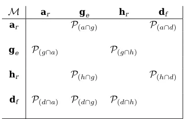
In the general case however, the set M con-sists of more elements, complicating the com-putation somewhat. Each x∈ Mmay share a number of supracontextual elements with other elements of M that have a different outcome. The situation may be as depicted in the follow-ing table, where columns are labelled by ele-ments ofM(in boldface) with their associated hypothetical outcomes (in italics).
Each cell in table 1 is associated with the power setP(x∩y). This power set is only com-puted if the outcome of x is not equal to the out-come of y, and both outout-comes are unique. The
M ar ge hr df
ar P(a∩g) P(a∩d)
ge P(g∩a) P(g∩h)
hr P(h∩g) P(h∩d)
df P(d∩a) P(d∩g) P(d∩h)
Table 1: Accessing disagreement inM × M
intersection is computed for all labels with a non-unique outcome, even for those with iden-tical outcomes. If two elements are non-unique, any label that is a subset of both will match up with their respective and disjoint data sets (see propositions 1 and 2 in (Johnsen and Jo-hansson, 2005)), thereby increasing the num-ber of disagreements, and consequently turn-ing any such label into a heterogeneous label. Note that a and h have the same outcome in this table making their intersective cells empty. Each non-empty cell corresponds to the sim-ple case above. The complication stems from the fact that different cells may have non-empty intersections, i.e., it is possible that
P(a∩g)∩ P(a∩d)6=∅
Arithmetic difference of the cardinality of the cells may be way off the mark, due to the pos-sibility that supracontexts may be subtracted more than once. Something more sophisticated is needed to compute the desired coefficients
cx. A couple of approximations are given in the
following.
The approximations are gotten at by first col-lecting all subcontexts different fromain a set
δ(a):
δ(a) ={x∈ M|o(a)6=o(x)}
This equation represents the column labels for the row fora.The total number of homogeneous supracontexts (=ca)more general thanais the
cardinality of the set difference
P(a)− [
x∈δ(a)
P(a∩x) (7)
more general than a, which also are shared with another subcontext, thus making all of them heterogeneous. The first term, Π(a), is the set of all supracontextual labels more gen-eral than a.Therefore, the difference between these two sets is equal to the collection of ho-mogeneous supracontextual labels more gen-eral than a. However, it is not the content of these sets that concerns us here; the goal is to find the cardinality of this difference.
The cardinality of P(a) is given the normal way as
kP(a)k= 2kak
but how are the behemoth union to be com-puted? This raises the question of computing the union of power sets:
[
x∈δ(a)
P(a∩x) (8)
The exponential order of the analogical algo-rithm lies in trying to compute this set. The union is bounded both from below and above. A lower bound is:
P(max({a∩x|x∈δ(a)})
and a higher bound is:
P( [
x∈δ(a)
a∩x)
Both these bounds are fairly simple to calcu-late. In the implementation (written in C), we have chosen a weighted average between the lower bound and the higher bound as a good approximation. We found that values that are weighted in favor of the higher bound gave bet-ter performance. This is not equivalent to say that the true AM values are closer to the higher bound.
3
Results from the
implementation
We have evaluated the performance of our implementation using the chunk identification task from CoNLL–2000 (Tjong Kim Sang and Buchholz, 2000). The best performance was ob-tained by a Support Vector Machine (Kudoh and Matsumoto, 2000, F=93.48). This implemen-tation has the disadvantage that it is computa-tionally very intensive, and it might not be ap-plicable to much larger data sets. Their results have later improved even more for the same
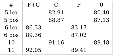
task. The standard for memory based learn-ing on this task is an F value of 91.54 (Veen-stra and Bosch, 2000), a value which can be im-proved upon slightly, as is shown by using a sys-tem combining several different memory-based learners (Tjong Kim Sang, 2000, F=92.5). Jo-hansson (2000) submitted an NGRAM model which used only 5 parts-of-speech tags , cen-tered around the item to be classified. That model (ibid.) used a backdown strategy to se-lect the largest context attested in the train-ing data, and gave the most frequent class of that context. It used a maximum of 4 look-ups from a table, and is most likely the fastest submitted model. The table could be created by sorting the database. The advantage be-ing that it could handle very large databases (as long as they could be sorted in reasonable time). The model gives a minimum baseline for what a modest N GRAM-model could achieve (F=87.23) on the chunking task.
only centering using both lexical and parts-of-speech features, and performs slightly bet-ter with feedback and cenbet-tering (F=92.05), al-though not as good as the SVM-implementation (Kudoh and Matsumoto, 2000), and not as good as the system combining several memory based learners (Tjong Kim Sang, 2000). A system that used 11 word features, and 11 parts-of-speech features, as well as a feedback feature was also trained, but did not perform better. The test-ing time for that 23-feature model was about 30 hours, making systematic testing difficult.
# F+C C F 0
5 lex 82.91 80.40
5 pos 88.87 87.13
6 lex 86.33 83.17 6 pos 89.36 87.02
10 91.16 89.48
11 92.05 89.41
Table 2: Results: F–scores. Number of features, Feedback + Centering, Centering only, Feed-back only, nothing extra.
3.1 Computational complexity
The test were made using a 867MHz PowerPC G4, with 1 MB L3 cache and 256 MB SDRAM memory using Mac OS X version 10.3.9. When the number of features changed, the number of unique patterns varied. The time to process all test patterns were therefor divided by the num-ber of unique database items and reported as how many milliseconds per database item the processing took. The results are shown in ta-ble 3. This shows an almost linear increase with the number of features, which has to do with a) that more comparisons are made because there are more features to compare, and b) that the match setMgrows faster when there are more features. When the size of the database is ac-counted for, the main contribution to complex-ity is proportional to the square of the size of the match set times the number of features. That complexity does not grow faster is an in-dication that the match set does not grow very fast for this task. However, when using 23 fea-tures, computing demanded more time than ac-counted for by the trend shown for less fea-tures. We speculate that this is mainly because of the limited RAM memory available. The val-ues in table 3 are approximated by the formula:
time = 0.05∗f2+f + 11.5, with R2 > 0.98; f = number of feature positions (variables), and time is in ms per database item, for processing all 49393 instances in the test set.
# D ms
5 lex 213532 17.44 5 pos 92392 17.84 6 lex 213562 19.14 6 pos 92392 19.80 10 213562 26.07 11 213591 28.68
Table 3: Results: Processing time needed to solve the full task, per item in the database.
4
Future research
We are trying to invent a method for automat-ically focussing on the relevant variables (fea-ture positions), set optimal weights for these variables. The goal is to get even better re-sults from this method, than from using the rather ad hoc weights used in this presentation. The focus on central variables reminds of the backdown strategy used in (Johansson, 2000), the results are very similar to that NGRAM– method for using only parts-of-speech informa-tion. The lexical information might be inte-grated in an NGRAM–model, weighted in an efficient way to produce results similar to the best results in this presentation (F=92.05), but without the computational overhead of the ana-logical model. The advantage of such a model is that it could use larger databases, and there-fore be much more practical, even if it does not deliver optimal results for smaller sets of data. Computation in the NGRAM–model (Johansson, 2000) consists of a fixed number of fast look-up operations, and training is feasible if the data can be sorted in reasonable time. Admittedly, non-naive implementations of a nearest neigh-bor model, such as TiMBL (Daelemans et al., 2004), are already doing well for large data sets, which make it hard to compete on com-bined accuracy and processing time.
5
Conclusion
detail elsewhere (Johnsen and Johansson, 2005; Johnsen, 2005). This reconstruction led to a more efficient approximation of full analogy modeling, and the results were implemented in a computer program, and tested on the
CoN LL−2000chunk tagging task. Our imple-mentation showed to be competitive with other memory based learners. An empirical confirma-tion of the computaconfirma-tional complexity showed a very slow increase with an increased number of features, although processing times increased with more demands on memory, an effect which is likely due to limits on internal memory.
We are presently not using feature weighting, such as information gain, which typically works on the level of individual feature values. Future research involves working on a method for au-tomatically finding the relevant variables, and finding optimal weights for these variables.
Acknowledgement Support by a grant
from the Norwegian Research Council under the KUNSTI programme (project BREDT) is kindly acknowledged. The computer program will be made available for download from http://bredt.uib.no with some example data.
References
S. Chandler. 1993. Are rules and modules re-ally necessary for explaining language? Jour-nal of Psycholinguistic Research, 22:593– 606.
S. Chandler. 2002. Skousen’s analogical ap-proach as an exemplar-based model of cate-gorization. InSkousen et al., pages 51–105.
W. Daelemans, J. Zavrel, K. van der Sloot, and A. van den Bosch. 2004. TiMBL: Tilburg Memory Based Learner, version 5.1. Refer-ence guide. ILK Technical report Series 04– 02., Tilburg, the Netherlands.
W. Daelemans. 2002. A comparison of analogi-cal modeling to memory-based language pro-cessing. InSkousen et al., pages 157–179.
D. Eddington. 2002. A comparison of two analogical models: Tilburg memory-based learner versus analogical modeling. In Sk-ousen et al., pages 141–155.
C. Johansson. 2000. A context sensitive max-imum likelihood approach to chunking. In Proceedings of CoNLL-2000 and LLL-2000, pages 136–138, Lisbon, Portugal.
L. Johnsen and C. Johansson. 2005. Efficient modeling of analogy. In A. Gelbukh, editor, Proceedings of the 6th Conference on Intelli-gent Text Processing and Computational Lin-guistics, volume 3406 of Lecture Notes in Computer Science, pages 682–691. Springer Verlag, Berlin, Germany.
L. Johnsen. 2005. Commentary on exegesis of Johnsen and Johansson, 2005. (ms.).
T. Kudoh and Y. Matsumoto. 2000. Use of support vector learning for chunk identifica-tion. InProceedings of CoNLL-2000 and LLL-2000, pages 142–144, Lisbon, Portugal.
M. Mudrow. 2002. Version spaces, neural net-works, and analogical modeling. InSkousen et al., pages 225–264.
J. Myers. 2002. Exemplar-driven analogy in op-timality theory. InSkousen et al., pages 265– 300.
J. Pierrehumbert. 2001. Exemplar dynam-ics: Word frequency, lenition, and contrast. In Frequency effects and the emergence of linguistic structure, pages 137–157, Amster-dam, the Netherlands. John Benjamins.
R. Skousen, D. Lonsdale, and D.B. Parkinson. 2002. Analogical Modeling: An exemplar-based approach to language, volume 10 of Human Cognitive Processing. John Ben-jamins, Amsterdam, the Netherlands.
R. Skousen. 1989. Analogical Modeling of Language. Kluwer Academic, Dordrecht, the Netherlands.
R. Skousen. 1992. Analogy and Structure. Kluwer Academic, Dordrecht, the Nether-lands.
R. Skousen. 2002. Issues in analogical model-ing. InSkousen et al., pages 27–48.
E.F. Tjong Kim Sang and S. Buchholz. 2000. Introduction to the CoNLL-2000 shared task: Chunking. In Proceedings of CoNLL-2000 and LLL-2000, pages 127–132, Lisbon, Por-tugal.
E.F. Tjong Kim Sang. 2000. Text chunking by system combination. In Proceedings of CoNLL-2000 and LLL-2000, pages 151–153, Lisbon, Portugal.